Estimating the significance of a signal in a multi-dimensional search

Abstract

In experiments that are aimed at detecting astrophysical sources such as neutrino telescopes, one usually performs a search over a continuous parameter space (e.g. the angular coordinates of the sky, and possibly time), looking for the most significant deviation from the background hypothesis. Such a procedure inherently involves a “look elsewhere effect”, namely, the possibility for a signal-like fluctuation to appear anywhere within the search range. Correctly estimating the $p$-value of a given observation thus requires repeated simulations of the entire search, a procedure that may be prohibitively expansive in terms of CPU resources. Recent results from the theory of random fields provide powerful tools which may be used to alleviate this difficulty, in a wide range of applications. We review those results and discuss their implementation, with a detailed example applied for neutrino point source analysis in the IceCube experiment.

1 Introduction

The statistical significance associated with the detection of a signal source is most often reported in the form of a $p$-value, that is, the probability under the background-only hypothesis of observing a phenomenon as or even more ‘signal-like’ than the one observed by the experiment. In many simple situations, a $p$-value can be calculated using asymptotic results such as those given by Wilk’s theorem [1], without the need of generating a large number of pseudo-experiments. This is not the case however when the procedure for detecting the source involves a search over some range, for example, when one is trying to observe a hypothetic signal from an astrophysical source that can be located at any direction in the sky. Wilk’s theorem does not apply in this situation since the signal model contains parameters (i.e. the signal location) which are not present under the null hypothesis. Estimation of the $p$-value could be then performed by repeated Monte Carlo simulations of the experiment’s outcome under the background-only hypothesis, but this approach could be highly time consuming since for each of those simulations the entire search procedure needs to be applied to the data, and to establish a discovery claim at the $5\sigma$ level ($p$-value=$2.87\times 10^{-7}$) the simulation needs to be repeated at least $\mathcal{O}(10^{7})$ times. Fortunately, recent advances in the theory of random fields provide analytical tools that can be used to address exactly such problems, in a wide range of experimental settings. Such methods could be highly valuable for experiments searching for signals over large parameter spaces, as the reduction in necessary computation time can be dramatic. Random field theoretic methods were first applied to the statistical hypothesis testing problem in [2], for some special case of a one dimensional problem. A practical implementation of this result, aimed at the high-energy physics community, was made in [3]. Similar results for some cases of multi-dimensional problems [4][5] were applied to statistical tests in the context of brain imaging [6]. More recently, a generalized result dealing with random fields over arbitrary Riemannian manifolds was obtained [7], openning the door for a plethora of new possible applications. Here we discuss the implementation of these results in the context of the search for astrophysical sources, taking IceCube [8] as a specific example. In section 2 the general framework of an hypothesis test is briefly presented with connection to random fields. In section 3 the main theoretical result is presented, and an example is treated in detail in section 4.

2 Formalism of a search as a statistical test

The signal search procedure can be formulated as a hypothesis testing problem in the following way. The null (background-only) hypothesis $H_{0}:\mu=0$, is tested against a signal hypothesis $H_{1}:\mu>0$, where $\mu$ represents the signal strength. Suppose that $\theta$ are some nuisance parameters describing other properties of the signal (such as location), which are therefore not present under the null. Additional nuisance parameters, denoted by $\theta^{\prime}$, may be present under both hypotheses. Denote by $\mathscr{L}(\mu,\theta,\theta^{\prime})$ the likelihood function. One may then construct the profile likelihood ratio test statistic [9]

$$q=-2\log\frac{\displaystyle\max_{\theta^{\prime}}\mathscr{L}(\mu=0,\theta^{\prime})}{\displaystyle\max_{\mu,\theta,\theta^{\prime}}\mathscr{L}(\mu,\theta,\theta^{\prime})}$$ (1)

and reject the null hypothesis if the test statistic is larger then some critical value. Note that when the signal strength is set to zero the likelihood by definition does not depend on $\theta$, and the test statistic (1) can therefore be written as

$$q=\displaystyle\max_{\theta\in\mathscr{M}}q(\theta)$$ (2)

where $q(\theta)$ is the profile likelihood ratio with the signal nuisance parameters fixed to the point $\theta$, and we have explicitely denoted by $\mathscr{M}$ the $D$-dimensional manifold to which the parameters $\theta$ belong. Under the conditions of Wilks’ theorem [1], for any fixed point $\theta$, $q(\theta)$ follows a $\chi^{2}$ distribution with one degree of freedom when the null hypothesis is true. When viewed as a function over the manifold $\mathscr{M}$, $q(\theta)$ is therefore a $\chi^{2}$ random field, namely a set of random variables that are continuously mapped to the manifold $\mathscr{M}$. To quantify the significance of a given observation in terms of a $p$-value, one is required to calculate the probability of the maximum of the field to be above some level, that is, the excursion probability of the field:

$$p\text{-value}=\mathbb{P}[\displaystyle\max_{\theta\in\mathscr{M}}q(\theta)>u].$$ (3)

Estimation of excursion probabilities has been extensively studied in the framework of random fields. Despite the seemingly difficult nature of the problem, some surprisingly simple closed-form expressions have been derived under general conditions, which allow to estimate the excursion probability (3) when the level $u$ is large. Such ‘high’ excursions are of course the main subject of interest, since one is interested in estimating the $p$-value for apparently significant (signal-like) fluctuations. We shall briefly describe the main theoretical results in the following section. For a comprehensive and precise definitions, the reader is referred to Ref. [7].

3 The excursion sets of random fields

The excursion set of a field above a level $u$, denoted by $A_{u}$, is defined as the set of points $\theta$ for which the value of the field $q(\theta)$ is larger than $u$,

$$A_{u}=\{\theta\in\mathscr{M}:q(\theta)>u\}$$ (4)

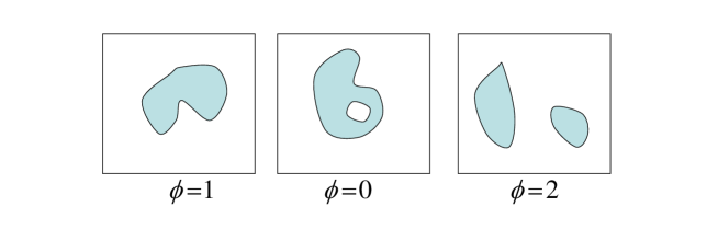
and we will denote by $\phi(A_{u})$ the Euler characteristic of the excursion set $A_{u}$. For a 2-dimensional field, the Euler characteristic can be regarded as the number of disconnected components minus the number of ‘holes’, as is illustrated in Fig.1. A fundamental result of [7] states that the expectation of the Euler characteristic $\phi(A_{u})$ is given by the following expression:

$$\mathbb{E}[\phi(A_{u})]=\sum_{d=0}^{D}\mathscr{N}_{d}\rho_{d}(u).$$ (5)

The coefficients $\mathscr{N}_{d}$ are related to some geometrical properties of the manifold and the covariance structure of the field. For the purpose of the present analysis however they can be regarded simply as a set of unknown constants. The functions $\rho_{d}(u)$ are ‘universal’ in the sense that they are determined only by the distribution type of the field $q(\theta)$, and their analytic expressions are known for a large class of ‘Gaussian related’ fields, such as $\chi^{2}$ with arbitrary degrees of freedom. The zeroth order term of eq. (5) is a special case for which $\mathscr{N}_{0}$ and $\rho_{0}(u)$ are generally given by

$$\mathscr{N}_{0}=\phi(\mathscr{M}),\hskip 14.22636pt\rho_{0}(u)=\mathbb{P}[q(\theta)>u]$$ (6)

Namely, $\mathscr{N}_{0}$ is the Euler characteristic of the entire manifold and $\rho_{0}(u)$ is the tail probability of the distribution of the field. (Note that when the manifold is reduced to a point, this result becomes trivial).

Figure 1: Illustration of the Euler characteristic of some 2-dimensional bodies.

When the level $u$ is high enough, excursions above $u$ become rare and the excursion set becomes a few disconnected hyper-ellipses. In that case the Euler characteristic $\phi(A_{u})$ simply counts the number of disconnected components that make up $A_{u}$. For even higher levels this number is mostly zero and rarely one, and Its expectation therefore converges asymptotically to the excursion probability. We can thus use it as an approximation to the excursion probability for large enough $u$ [10]

$$\mathbb{E}[\phi(A_{u})]\approx\mathbb{P}[\displaystyle\max_{\theta\in\mathscr{M}}q(\theta)>u].$$ (7)

The practical importance of Eq. (5) now becomes clear, as it allows to estimate the excursion probabilities above high levels. Furthermore, the problem is reduced to finding the constants $\mathscr{N}_{d},d>0$. Since Eq. (5) holds for any level $u$, this could be achieved simply by calculating the average of $\phi(A_{u})$ at some low levels, which can be done using a small set of Monte Carlo simulations. We shall now turn to a specific example where this procedure is demonstrated.

4 Application to neutrino source detection

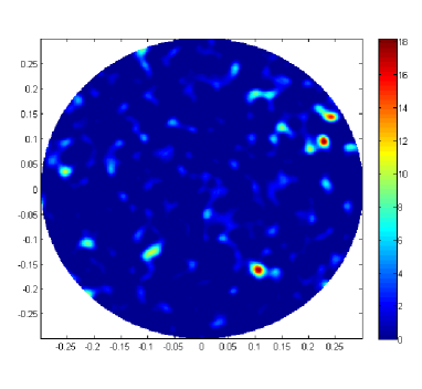
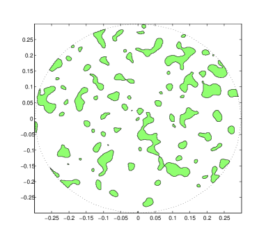
The IceCube experiment [8] is a neutrino telescope located at the south pole and aimed at detecting astrophysical neutrino sources. The detector measures the energy and angular direction of incoming neutrinos, trying to distinguish an astrophysical point-like signal from a large background of atmospheric neutrinos spread across the sky. The nuisance parameters over which the search is performed are therefore the angular coordinates $(\theta,\varphi)$. We follow [11] for the definitions of the signal and background distributions and the likelihood function. The signal is assumed to be spatially Gaussian distributed with a width corresponding to the instrumental resolution of $0.7^{o}$, and the background from atmospheric neutrinos is assumed to be uniform in azimuthal angle. We use a background simulation sample of 67000 events, representing roughly a year of data, provided to us by the authors of [11]. We then calculate a profile likelihood ratio as described in the previous section. Figure 2 shows a “significance map” of the sky, namely the values of the test statistic $q(\theta,\varphi)$ as well as the corresponding excursion set above $q=1$. To reduce computation time we restrict here the search space to the portion of the sky at declination angle 27^∘ below the zenith, however all the geometrical features of a full sky search are maintained. Note that the most significance point has a value of the test statistic above 16, which would correspond to a significance exceeding 4$\sigma$ if this point would have been analyzed alone, that is without the “look elsewhere” effect.

Figure 2: (a) A significance map showing a projection of the test statistic $q(\theta,\varphi)$ for a background simulation (b) The corresponding excursion set above $q=1$. The Euler characteristic in this example is 95.

4.1 Computation of the Euler characteristic

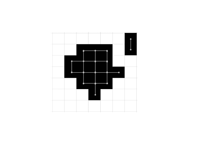
In practice, the test statistic $q(\theta,\varphi)$ is calculated on a grid or points, or ‘pixels’, which are sufficiently smaller than the detector resolution. The computation of the Euler characteristic can then be done in a straightforward way, using Euler’s formula:

$$\phi=V-E+F$$ (8)

where $V$, $E$, and $F$ are respectively the numbers of vertices (pixels), edges and faces making up the excursion set. An edge is a line connecting two adjacent pixels and a face is the square made by connecting the edges of four adjacent pixels. An Illustration is given Fig.3. (Although it is most convenient to use a simple square grid, other grid types can be used if necessary, in which case the faces would be of other polygonal shapes).

Figure 3: Illustration of the computation of the Euler characteristic using formula (8). Each square represents a pixel. Here, the number of vertices is 18, the number of edges is 23 and the number of faces is 7, giving $\phi=18-23+7=2$.

Once the Euler characteristic is calculated, the coefficients of Eq. (5) can be readily estimated. For a $\chi^{2}$ random field with one degree of freedom and for two search dimensions, the explicit form of Eq. (5) is given by [7]:

$$\mathbb{E}[\phi(A_{u})]=\mathbb{P}[\chi^{2}>u]+e^{-u/2}(\mathscr{N}_{1}+\sqrt{u}\mathscr{N}_{2}).$$ (9)

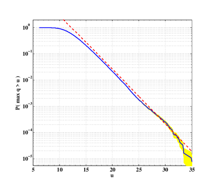
To estimate the unknown coefficients $\mathscr{N}_{1},\mathscr{N}_{2}$ we use a set of 20 background simulations, and calculate the average Euler characteristic of the excursion set corresponding to the levels $u=0,1$ (The number of required simulations depends on the desired accuracy level of the approximation. For most practical purposes, estimating the $p$-value with a relative uncertainty of about 10% should be satisfactory.). This gives the estimates $\mathbb{E}[\phi(A_{0})]=33.5\pm 2$ and $\mathbb{E}[\phi(A_{1})]=94.6\pm 1.3$. By solving for the unknown coefficients we obtain $\mathscr{N}_{1}=33\pm 2$ and $\mathscr{N}_{2}=123\pm 3$. The prediction of Eq. (9) is then compared against a set of approx. 200,000 background simulations, where for each one the maximum of $q(\theta,\varphi)$ is found by scanning the entire grid. The results are shown in Figure 4. As expected, the approximation becomes better as the $p$-value becomes smaller. The agreement between Eq. (9) and the observed $p$-value is maintained up to the smallest $p$-value that the available statistics allows us to estimate.

Figure 4: The prediction of Eq. (9) (dashed red) against the observed $p$-value (solid blue) from a set of 200,000 background simulations. The yellow band represents the statistical uncertainty due to the available number of background simulations.

4.2 Slicing the parameter space

A useful property of Eq. (5) that can be illustrated by this example, is the ability to consider only a small ‘slice’ of the parameter space from which the expected Euler characteristic (and hence $p$-value) of the entire space can be estimated, if a symmetry is present in the problem. This can be done using the ‘inclusion-exclusion’ property of the Euler characteristic:

$$\phi(A\cup B)=\phi(A)+\phi(B)-\phi(A\cap B).$$ (10)

Since the neutrino background distribution is assumed to be uniform in azimuthal angle ($\varphi$), we can divide the sky to $N$ identical slices of azimuthal angle, as illustrated in Figure 5. Applying (10) to this case, the expected Euler characteristic is given by

$$\mathbb{E}[\phi(A_{u})]=N\times(\mathbb{E}[\phi(slice)]-\mathbb{E}[\phi(edge)])+\mathbb{E}[\phi(0)]$$ (11)

where an ‘edge’ is the line common to two adjacent slices, and $\phi(0)$ is the Euler characteristic of the point at the origin (see Figure 5).

Figure 5: Illustration of the excursion set in a slice of a sky, showing also an edge (solid blue) and the origin as defined in Eq. (11). In this example $\phi(slice)=6$, $\phi(edge)=2$ and $\phi(0)=0$.

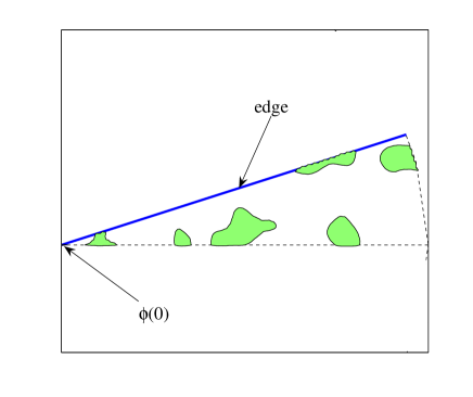
We can now apply Eq. (5) to both $\phi(slice)$ and $\phi(edge)$ and estimate the corresponding coefficients as was done before, using only simulations of a single slice of the sky. Following this procedure we obtain for this example with $N=18$ slices from 40 background simulations, $\mathscr{N}_{1}^{slice}=6\pm 0.5,\mathscr{N}_{2}^{slice}=6.7\pm 0.8$ and $\mathscr{N}_{1}^{edge}=4.4\pm 0.2$. Using (11) this leads to the full sky coefficients $\mathscr{N}_{1}=28\pm 9$ and $\mathscr{N}_{2}=120\pm 14$, a result which is consistent with the full sky simulation procedure. This demonstrates that the $p$-value can be accurately estimated by only simulating a small portion of the search space.

5 Summary

The Euler characteristic formula, a fundamental result from the theory of random fields, provides a practical mean of estimating a $p$-value while taking into account the “look elsewhere effect”. This result might be particularly useful for experiments that involve a search for signal over a large parameter space, such as high energy neutrino telescopes. While the example considered here deals with a search in a 2-dimensional space, the formalism is general and could be in principle applied to any number of search dimensions. For example, if one is trying to detect a ‘burst’ event then time would constitute an additional search dimension. In such case the method of slicing could be useful as well, as one will not have to simulate the entire operating period of the detector but only a small ’slice’ of time (provided that the background does not vary in time). Thus, the computational burden of having to perform a very large number of Monte Carlo simulations in order to to estimate a $p$-value, could be greatly reduced.

6 Acknowledgments

We thank Jim Braun and Teresa Montaruli for their help in providing us the background simulation data of IceCube which was used to perform this analysis. One of us (E. G.) is obliged to the Minerva Gesellschaft for supporting this work.

References

- [1] S.S. Wilks, The large-sample distribution of the likelihood ratio for testing composite hypotheses, Ann. Math. Statist. 9 (1938) 60-62.
- [2] R.B. Davies, Hypothesis testing when a nuisance parameter is present only under the alternative., Biometrika 74 (1987), 33-43.
- [3] E. Gross and O. Vitells, Trial factors for the look elsewhere effect in high energy physics , Eur. Phys. J. C, 70 (2010), 525-530.
- [4] R.J. Adler and A.M. Hasofer, Level Crossings for Random Fields,Ann. Probab. 4, Number 1 (1976), 1-12.
- [5] R.J. Adler, The Geometry of Random Fields, New York (1981), Wiley, ISBN: 0471278440.
- [6] K.J. Worsley, S. Marrett, P. Neelin, A.C. Vandal, K.J. Friston and A.C. Evans, A Unified Statistical Approach for Determining Significant Signals in Location and Scale Space Images of Cerebral Activation, Human Brain Mapping 4 (1996) 58-73.
- [7] R.J. Adler and J.E. Taylor, Random Fields and Geometry , Springer Monographs in Mathematics (2007). ISBN: 978-0-387-48112-8.
- [8] J. Ahrens et al. and The IceCube Collaboration, Astropart. Phys. 20 (2004), 507.
- [9] G. Cowan, K. Cranmer, E. Gross and O. Vitells, Asymptotic formulae for likelihood-based tests of new physics, Eur. Phys. J. C 71 (2011) 1544, [arXiv:1007.1727].
- [10] J. Taylor, A. Takemura and R.J. Adler, Validity of the expected Euler characteristic heuristic, Ann. Probab. 33 (2005) 1362-1396.
- [11] J. Braun, J. Dumma, F. De Palmaa, C. Finleya, A. Karlea and T. Montaruli, Methods for point source analysis in high energy neutrino telescopes, Astropart. Phys. 29 (2008) 299-305 [arXiv:0801.1604].