The RMS Survey: Critical Tests of Accretion Models for the Formation of Massive Stars
Abstract
There is currently no accepted theoretical framework for the formation of the most massive stars, and the manner in which protostars continue to accrete and grow in mass beyond 10⊙ is still a controversial topic. In this study we use several prescriptions of stellar accretion and a description of the Galactic gas distribution to simulate the luminosities and spatial distribution of massive protostellar population of the Galaxy. We then compare the observables of each simulation to the results of the Red MSX Source (RMS) survey, a recently compiled database of massive young stellar objects. We find that the observations are best matched by accretion rates which increase as the protostar grows in mass, such as those predicted by the turbulent core and competitive accretion (i.e. Bondi-Hoyle) models. These ‘accelerating accretion’ models provide very good qualitative and quantitative fits to the data, though we are unable to distinguish between these two models on our simulations alone. We rule out models with accretion rates which are constant with time, and those which are initially very high and which fall away with time, as these produce results which are quantitatively and/or qualitatively incompatible with the observations. To simultaneously match the low- and high-luminosity YSO distribution we require the inclusion of a ‘swollen-star’ pre-main-sequence phase, the length of which is well-described by the Kelvin-Helmholz timescale. Our results suggest that the lifetime of the YSO phase is yrs, whereas the compact Hii-region phase lasts between yrs depending on the final mass of the star. Finally, the absolute numbers of YSOs are best matched by a globally averaged star-formation rate for the Galaxy of 1.5-2⊙yr-1.
keywords:
stars: massive, stars: pre-main-sequence, stars: protostars, stars: formation1 Introduction
The formation mechanism for stars with masses 10⊙ is still unclear. The steepness of the Initial Mass Function (IMF) means that such stars are rare, while the short Kelvin-Helmholz contraction times of massive stars mean that they arrive on the main-sequence (MS) whilst still accreting and heavily embedded within their natal molecular clouds. Meanwhile, from a theoretical point-of-view there is considerable doubt that the ‘classical’ theory of star formation is applicable massive stars. Firstly, in the model of an isothermal collapsing sphere, the accretion rate depends only on the sound-speed of the gas (Shu, 1977), and implies unrealistically large formation timescales for stars with masses 10⊙ (Stahler et al., 2000). Secondly, once the massive proto-star arrives on the MS it will exert considerable outward radiation pressure on the infalling material. In the spherically-symmetric case, this can impede and eventually halt accretion, preventing the formation of a high-mass star (Kahn, 1974; Wolfire & Cassinelli, 1987). For further discussions regarding both the theoretical and observational challenges faced in the study of massive star formation, see Zinnecker & Yorke (2007).
There are several proposed amendments to the classical model of star formation to account for massive stars, a few of which we now discuss. McKee & Tan (2003, hereafter MT03) suggested a mechanism whereby the larger molecular pre-stellar cores are supported against collapse by larger turbulent motions (the turbulent core model). Once these cores become unstable to collapse they have accretion rates which accelerate with time. In the competitive accretion model (Bonnell & Bate, 2006), a large reservoir of gas is funnelled to the centre of a cluster of protostars, allowing the cores at the cluster’s centre to achieve very large accretion rates through the Bondi-Hoyle mechanism. Schmeja & Klessen (2004) proposed that the accretion rates of proto-stars within a gas cloud are governed by the complex interplay of self-gravity and turbulence, and that upon collapse they have initially very high accretion rates owing to the large amounts of material that has accumulated in their immediate viscinity (the gravo-turbulent model). Indeed, several authors have proposed models for star formation in which accretion rates behave in this way with time (Foster & Chevalier, 1993; Whitworth & Ward-Thompson, 2001; Motoyama & Yoshida, 2003). Meanwhile, 3-D hydrodynamical simulations of massive forming stars through accretion from a circumstellar disk displayed accretion rates which were approximately constant throughout the simulation, though they may pass through distinct accretion phases and be highly variable on short timescales (Krumholz et al., 2009; Kuiper et al., 2011).
The mechanisms described above predict accretion rates which evolve differently throughout the formation timescale of the star. The turbulent core and competitive accretion (Bondi-Hoyle) models, though they differ in form, both predict accretion rates that should accelerate with time as the central star grows in mass. The gravo-turbulent model however predicts that there should be an initial burst of accretion, which gradually tails off as the star approaches its final mass. These can be contrasted to the ‘standard model’ of star-formation, as well as those found in the numerical simulations of Krumholz et al. (2009) and Kuiper et al. (2011), when the accretion rate is largely constant. As the accretion rate and its evolution will govern the proto-star’s luminosity as a function of time, as well as the star’s formation timescale, with a large complete sample of massive forming stars it should be possible to distinguish between these scenarios from analysis of their luminosity distribution.
1.1 The RMS Survey
Such a sample has recently come to fruition. The Red MSX Source (RMS) survey (Hoare et al., 2005)111http://www.ast.leeds.ac.uk/RMS has selected point-sources from the MSX catalogue (Egan et al., 2003) with colours appropriate for young massive stars (Lumsden et al., 2002), and weeded out contaminant objects such as planetary nebulae and evolved stars through follow-up near-infrared spectroscopy and continuum radio observations (Urquhart et al., 2007a, 2009b). Sources have kinematic distance estimates from molecular line observations (Urquhart et al., 2007b, 2008, 2009a), while the sources’ bolometric luminosities have been determined from fits to their spectral energy distributions (Mottram et al., 2011b). High-resolution mid-infrared imaging has been used to investigate source multiplicity (Mottram et al., 2007). The RMS database now contains over 1,000 confirmed massive young stars. These objects are separated into massive Young Stellar Objects (YSOs) and compact Hii-regions based on one of two criteria. Objects which are spatially extended in the high resolution mid-infrared images (spatial resolution 1′′) due to Lyman- heating of the surrounding dust, or which have detectable radio emission (1mJy/beam) are considered to be ionizing their surroundings, and hence are classified as Hii-regions. These objects are considered to have reached the main-sequence, though they may still be accreting. Objects displaying no evidence for an ionized nebula are classified as YSOs.
In this paper we use the results of the RMS survey to test the predictions of different accretion laws. We do this by constructing realistic populations of massive protostars and distributing them throughout the Galaxy according to a model of the Galaxy’s gas distribution. We compute the observed properties of the objects in the simulation, apply the RMS selection and classification criteria and compare them to the observed results.
This paper is similar in concept to that of Froebrich et al. (2006), who used the numerical results of Schmeja & Klessen (2004) to make predictions about the earliest stages of star formation. It is also similar to Robitaille & Whitney (2010), who calculated the evolution of the spectral energy distribution (SED) of intermediate mass YSOs ⋆5-10⊙ using a single accretion law. From this, they calculated the predicted fluxes in the four Spitzer/IRAC channels and compared the total number of objects to those found in the GLIMPSE survey. They then used this information to predict the global star-formation rate of the Galaxy. Our approach is different, in that we predict the 21µm luminosity function of massive YSOs for a variety of different accretion scenarios, with the ultimate goal of understanding how massive stars form, although we too are able to put some constraints on the Galactic global star-formation rate.
We begin in Sect. 2 with a description of the model construction. The results of the model, the effect of the free parameters, and of the different accretion laws, are presented in Sect. 3. We discuss the results and the implications for models of massive star formation in Sect. 4. We provide a summary of our results in Sect. 5.
2 Model construction
The methodology for the construction of the model is as follows: assuming a global star formation rate of the Galaxy, we generate yrs of stars – up until the point where the oldest massive stars have comfortably reached the main-sequence and have broken free of their natal environments. Using a description of the gas distribution in the Galaxy, these stars are each inserted into the model Galaxy at a random location dictated by the relation between local gas density and local star-formation rate. That is, locations of high density have higher star formation rates, and hence are more likely to host newly-formed stars. Quantitatively, we scale the star-formation rate with gas density SFR, in accordance with the Schmidt-Kennicutt law for star-forming galaxies (Kennicutt, 1998). Typically, the value of is quoted, though some authors have suggested that is closer to unity, and may even be as low as 0.8 (Blanc et al., 2009). Strictly this law applies to the surface density of galaxies, but since the scale height of the Galaxy’s gas distribution is small compared to the radial size, .
Each star in the simulation is given an age (i.e. time since accretion first began), which is randomly selected from a uniform distribution between 0 – yrs. Using a given model of stellar accretion, the age, and final mass fin of each star, we compute the current mass cur. The pre-main-sequence birthlines of Hosokawa & Omukai (2009) are then used to compute the luminosities of each star, which we then use to calculate the observed flux at 21µm. For stars which we determine have arrived on the main-sequence, making standard assumptions we calculate the properties of the surrounding Hii-region, and ultimately the observed radio flux. We then pass the observables through the RMS selection criteria, and those sources which would be detected in the survey are then classified according to their observed properties. Below, each step of the process is described in more detail.
2.1 Galactic gas distribution
For a prescription of the distribution of baryonic material in the Galaxy, we use as a basis the Galactic distribution of free electrons as determined by Taylor & Cordes (1993, and refs therein), and later updated by Cordes & Lazio (2002) in a model known as NE2001. These studies use pulsars with known distances to infer the line-of-sight density of free electrons. We assume that in the Milky Way disk, the total ISM density (neutral gas, dust etc.) scales directly with the density of free electrons.
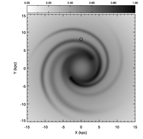
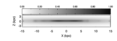
The model consists of three components: thin disk, thick disk, and four spiral arms. For the thin and thick disk components we use the definitions and physical parameters as defined in NE2001. For the spiral arms, we have made slight adjustments: we used the coordinates of the fiducial points for each of the four arms as quoted by TC93 and fitted each arm with a logarithmic spiral,
| (1) |
where and define the Galactocentric distance and azimuthal angle222 is defined as the Sun - Galactic Centre axis. of each spiral arm ; and are fitted constants; and is the minimum Galactocentric radius of the defining fiducial points in TC93. We specified that two spiral arms should originate from the ends of the central Bar. To ensure this we adjusted the fiducial points such that was always 4kpc (the length of the Bar as determined by Benjamin et al., 2005) and was 45° for the Scutum-Crux arm and 225° for the opposing (Perseus) arm. The other two arms (Sagittarius and Norma) were traced inwards according to the logarithmic fit, and the inner regions of the arms were attenuated to blend with the inner disk component using an attenuation function , similar to that used in the NE2001 model;
We used a somewhat arbitrary value of 5kpc for in order to blend them with the inner thin disk. For the outer disk, the spiral arms were extrapolated radially outwards to 21kpc, at which point their contribution to the local gas density is negligible. The normalised surface density of the Galaxy gas distribution model in both the and planes can be seen in Fig. 1.
The description of the Galactic gas density we use has not been precisely tuned to the current state-of-the-art picture of our Galaxy’s morphology. For example, we do not include the ‘kinks’ in the arms in the Solar neighbourhood, nor do we include other smaller features such as the ‘local’ arm. Our goal here is not to accurately predict the spatial distribution of the YSO population, nor is it to trace the spiral structure of our Galaxy. The purpose of this work is to model the observed luminosity distributions of protostars, and so we only need a description of the Galaxy’s morphology which is realistic in terms of size-scales (e.g. the scale-height, ) and discrete structures (e.g. the number and size-scales of spiral arms). Tweaks that we could make to the model gas distribution to better match the spatial distribution will be discussed later, while a better match to the 3-dimensional distribution of young massive stars awaits the implementation of more accurate distances (see e.g. Reid et al., 2009).
2.2 Generation of stellar populations
Assuming a global star-formation rate for the Galaxy of SFRGal, we generate 1Myr of star-formation, under the assumption that any star older than 1Myr would be sufficiently free of its natal material to be precluded by the RMS selection criteria as being too evolved. Estimates of SFRGal range from 2-10⊙yr-1, though most measurements appear to be in the range 3-4⊙yr-1 (see Diehl et al., 2006, and references therein). Recently, in a study which was similar to the one presented here, Robitaille & Whitney (2010) attempted to derive SFRGal from a sample of YSOs selected from GLIMPSE, finding that values of SFRGal=0.7-1.5⊙yr-1 were preferred. This is somewhat lower than the other estimates described above. However, Robitaille & Whitney (2010) used only one description of accretion history in their study, that of Bernasconi & Maeder (1996), though it is unclear whether they used the constant accretion rates or those that increased with protostellar mass (see Robitaille et al., 2006). In either case, these accretion rates of Bernasconi & Maeder (1996) are an order of magnitude lower than those presented in more contemporary studies of e.g. MT03. This produces slightly longer pre-MS lifetimes and therefore results in larger numbers of YSOs. This may explain in part why Robitaille & Whitney (2010) required values of SFRGal which were lower than in previous studies. For now we adopt SFRGal=3⊙yr-1. This parameter affects only the overall normalization of objects, and the effect on our conclusions of allowing this parameter to vary slightly will be explored later.
For the total mass of stars in our model, we generate a distribution of stellar masses according to the Initial Mass Function (IMF) of Kroupa (2001), which is essentially the Salpeter law but augmented at low masses. The masses we generate are the final stellar masses fin, i.e. the mass that each star will have once it has finished accreting. We make the assumption that the global star formation rate has been constant over the last 106yrs, and the age of each star in the simulation is selected from a uniform random distribution of ages from zero to 106yrs. We did experiment with ‘clustering’ the star formation into localized bursts, which is likely to be a more realistic representation of how star formation proceeds within the Galaxy, but this was found to have no impact on the results other than to increase stochastic effects within a single simulation.
2.3 Computation of observables
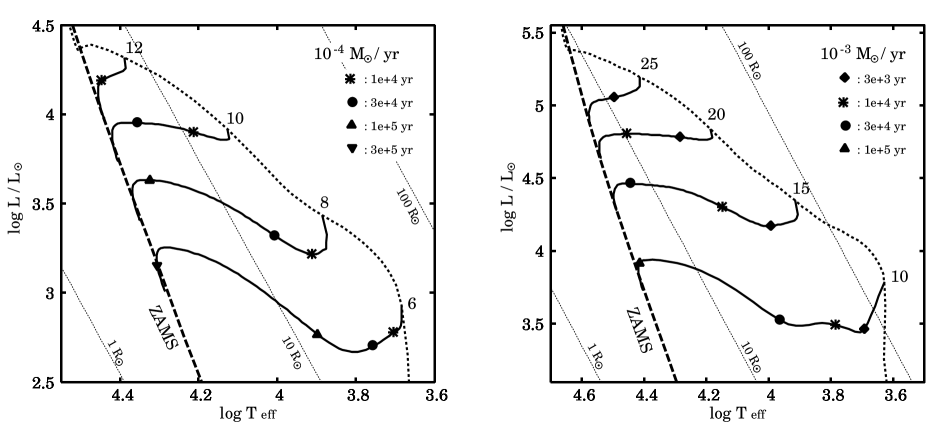
In order to calculate the observed properties of the protostars in our simulations, we utilize the theoretical evolution tracks for accreting protostars taken from Hosokawa & Omukai (2009, hereafter HO09). The authors calculated the evolution of accreting protostars for various constant accretion rates. They show that the evolution with high accretion rates of has some characteristic features. With , for example, the protostar becomes significantly swollen and does not reach the main-sequence (MS) for . The critical mass becomes higher with the higher accretion rate. If the mass accretion ceases before the arrival to the MS, the star experiences a contraction phase lasting approximately a Kelvin-Helmholtz timescale ,
| (2) |
This predicts that massive pre-main-sequence (PMS) stars exceeding should exist. Figure 2 shows the evolution tracks for such massive PMS stars in the HR diagram. In this paper, we assume that the massive PMS stars contract keeping the constant luminosity for simplifying the detailed evolution.
2.3.1 Accretion laws
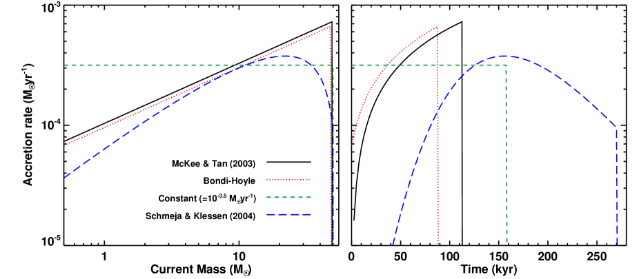
To calculate the physical properties of the forming star, we must first know how much matter has been accreted since the star began to form. For this, we require a prescription of the star’s accretion rate. In this study we investigate three distinct accretion-rate scenarios: constant accretion-rate; accretion-rates which increase as the mass of the star grows; and those which decrease. Below, we describe the prescriptions for each of these accretion rates, while in Fig. 3 we illustrate the behaviour of the accretion rates with both mass and time for each of these laws.
a) Constant accretion
Here we use the results of HO09 directly. For the age and final mass fin of each star in our simulation, we calculate the current mass for a specified accretion rate from,
| (3) |
We can also calculate the formation timescale of the star from,
| (4) |
We use the HO09 tracks to calculate the luminosity and temperature of each star from its current mass cur. For stars which have reached their final mass but whose masses are below the for that accretion rate, we calculate the Kelvin-Helmholz timescale . If a star is not older than then it is considered to still be ‘swollen’, that is it has not yet contracted to the main-sequence, and so emits a negligible amount of ionizing flux. Stars which have arrived on the main-sequence are considered to have Lyman fluxes similar to zero-age main-sequence stars of the same mass, but with extra luminosity due to accretion.
b) Accelerating accretion I: MT03
In the MT03 prescription of accretion by a massive protostar in the turbulent core model, the accretion rate and formation timescale form of an accreting star are given by their Equs. (41) and (44),
| (5) |
| (6) |
where is the surface density of a prestellar clump in units of g cm-2. From these equations we can find an expression for the current mass of an accreting star,
| (7) |
Using these equations, and the randomly generated stellar ages, we can then calculate the current mass and formation timescale of each star.
To calculate the luminosities of the accreting star, we must take into account the stellar luminosity and the accretion luminosity. To do this we take the star’s current mass and current accretion rate, and look up the corresponding luminosity from the tracks of HO09. In doing so, we are making two approximations: firstly, we linearly interpolate the HO09 tracks in log-space at 0.01dex increments between 10-5 and 10-3⊙yr-1, since HO09 only calculate tracks at 10-3, 10-4 and 10-5⊙yr-1. Secondly, we are assuming that a star whose accretion rate has accelerated to the current value has a similar luminosity to a star whose accretion rate has always been constant at the current value. While one may expect there to be systematic differences between these two cases, we found that the cur-bol relationship of our approximation was quantitatively similar to that computed by MT03 (their Fig. 6), since the accretion luminosity only contributes a small fraction to the total luminosity.
For stars which have finished accreting, luminosties are taken from the stellar structure models of Meynet & Maeder (2000).
Again, MT03 find that very massive stars join the MS at 20⊙, though the precise value of depends on . As with the case of constant accretion, stars which have finished accreting but have final masses below are assumed to undergo a pre-MS contraction phase which approximates to for that particular star.
c) Accelerating accretion II: Bondi-Hoyle accretion
Similar accelerating accretion is predicted under the Bondi-Hoyle (BH) accretion relevant to the competitive accretion model (Bonnell & Bate, 2006). The difference here is that the accretion rate depends only on and cur, not on fin. The BH accretion rate is given by Equ. (6) of Bonnell & Bate (2006),
| (8) |
where and are the velocity dispersion and gas density within the star-forming clump, and is the initial mass of a star-forming clump that becomes unstable to gravitational collapse. Integrating and rearranging this equation, and using the values determined by Bonnell & Bate (2006) for the parameters of , and (0.5 km s-1, 10-17g cm3, and 0.5⊙ respectively), the current mass of a star accreting in this way can be shown to be given by,
| (9) |
The formation timescale is then simply,
| (10) |
There has yet to be a thorough computation of BH birthlines, so we must make assumptions for the object’s luminosity, the duration of the pre-MS ‘swollen’ phase and the mass at which very massive stars arrive on the MS, MS. The luminosity of a BH accreting object is again assumed to be well represented by the HO09 track with the same current accretion rate at the same cur. We again assume that the MS contraction time is equal to , and we leave MS as a free parameter in this model.
d) Decelerating accretion
For a representitive model of decelerating accretion, we use the ‘gravo-turbulent fragmentation’ model of Schmeja & Klessen (2004, hereafter SK04). In this model, protostars at the centre of a cluster’s potential well are subject to a greater amount of infalling material, and the initial accretion rates are very high. As the reservoir of material is depleted, the accretion-rate gradually decreases, eventually falling to zero. Before preceeding with a description of how we incorporate this accretion scenario into our simulations, we first note that in SK04 no stars more massive that 10⊙ are formed, and that these authors’ goals were not necessarily to simulate massive star formation. Nevertheless, we include it in our study as a tool with which to examine how decelerating accretion affects the relative numbers of massive protostars.
For a prescription of such accretion, we use the recipes of SK04, which are taken from empirical fits to their numerical simulations. Here the accretion rate is given by,
| (11) |
where 0 and are constants. The constant 0 specifies the maximum accretion rate, which is reached after a brief period of rapid acceleration in . Once the accretion rate reaches 0, it falls away gradually on a timescale dictated by .
As a representative case of decelerating accretion, we use the simulation ‘G2’ from SK04, which uses a gaussian realization of the initial turbulence within the molecular cloud. Here, the value of 0 was found to be a linear function of fin, up to fin10⊙. Specifically, from fits to their data,
| (12) |
Though SK04 formed no stars with masses greater than 10⊙, for our simulations we make the simple assumption that this relation can be extrapolated up to the most massive stars in our simulation, fin=150⊙. The parameter also appears to be a linear function of fin, though there is considerable dispersion in this relation. From our linear fits to the results of SK04, we find,
| (13) |
with,
Therefore, for a star of given fin and age , Eqs. (11), (12) and (13) can be used to calculate that star’s accretion rate as a function of time since =0. Integration of this function then yields the star’s current mass cur.
Using these parameters however, the formation times of massive stars become unrealisticly long, and no stars with fin15⊙ can be formed within 106yrs. Massive stars can be formed within a reasonable time, but only if the constants in Eq. (13) are pushed to their extreme limits, such that the largest possible values of result. This will be discussed further in Sect. 4.
As with the other accretion laws studied, luminosities are determined from the pre-MS tracks of HO09, MS is left as a free parameter, and the length of the pre-MS ‘swollen’ phase is assumed to be given by the KH timescale.
2.3.2 21µm luminosity
Having calculated bol from the accretion law, we can now determine the observed flux through the MSX 21m filter, one criterion used for source selection in the RMS survey. In Mottram et al. (2011b) it was found that the 21µm flux of objects in the sample scaled as a constant fraction of the total bolometric flux according to,
| (14) |
No significant correlation was found between and any observable parameter in the RMS survey, such as IR colour or .
To convert our determined in in Sect. 2.3.1 to , we use the following relation,
| (15) |
where is randomly drawn from a normal distribution of numbers with a mean of 1.43 and standard deviation of 0.27 (following Eq. 14); is the interstellar extinction (see below), and is the effective bandwidth of the MSX 21µm filter.
As yet we have not dealt exlicitly with the issue of line-of-sight extinction. There are likely two sources of extinction to each source – interstellar, and circumstellar. Circumstellar extinction will vary largely from source to source, since it will depend on random properties such as cavity opening angle and inclination to line-of-sight. We have assumed that the factor incorporates the attenuating effect of circumstellar extinction.
In terms of interstellar extinction at 21m towards each object, , one may expect a systematic trend of this factor with object distance. We have made a detailed study of this factor and how it may impact our results, using Galactic star clusters as test points (see Appendix A). Though we do account for this effect by incorporating a factor of into Eq. 15, we expect at most that this plays a very minor role in the results of our simulation, since for even the most distant objects.
The current model does not account for a mid-IR faint or ‘dark’ phase early on in the evolution of massive stars. Examples of luminous young objects that are mid-IR faint/dark clearly do exist. Ellingsen (2006) found that 30% of methanol maser sources, that are invariably associated with massive YSOs, do not have counterparts in the 4-8 micron GLIMPSE survey. Also, about 20% of the active cores in infrared dark clouds (IRDCs) have a luminosity greater than 5000⊙ (Rathborne et al., 2010). Though we are not yet explicitly accounting for an IR ‘dark’ phase here, during the very early stages of the growth of massive stars their luminosity will be below 5000⊙ and therefore not in the RMS survey; an aspect that is already accounted for in the modelling presented here. Since very few IR-dark YSOs have luminosities that would impact on our analysis, we neglect such objects in this current work.
| Mass | Teff | Log (L⋆/⊙) | R⋆ | BCV | MV | Log | tKH |
|---|---|---|---|---|---|---|---|
| (⊙) | (K) | (⊙) | (phot s-1) | (103yrs) | |||
| 6 | 19000 | 3.01 | 3.0 | -1.83 | -0.95 | 43.33 | 367.1 |
| 9 | 22895 | 3.57 | 3.9 | -2.28 | -1.89 | 44.76 | 175.5 |
| 12 | 26743 | 3.96 | 4.5 | -2.64 | -2.52 | 46.02 | 107.8 |
| 15 | 29783 | 4.26 | 5.1 | -2.88 | -3.01 | 47.03 | 76.2 |
| 20 | 33824 | 4.61 | 6.0 | -3.22 | -3.56 | 48.00 | 51.8 |
| 25 | 36831 | 4.86 | 6.7 | -3.47 | -3.93 | 48.46 | 40.2 |
| 30 | 38670 | 5.02 | 7.3 | -3.61 | -4.19 | 48.69 | 36.7 |
| 35 | 40596 | 5.18 | 8.0 | -3.75 | -4.45 | 48.90 | 31.7 |
| 40 | 42610 | 5.34 | 8.7 | -3.89 | -4.71 | 49.09 | 26.3 |
| 50 | 44589 | 5.52 | 9.8 | -4.03 | -5.02 | 49.31 | 24.1 |
| 60 | 46647 | 5.70 | 11.0 | -4.18 | -5.33 | 49.43 | 20.4 |
| 70 | 47662 | 5.81 | 12.0 | -4.25 | -5.53 | 49.51† | 19.7 |
| 80 | 48694 | 5.92 | 13.1 | -4.32 | -5.74 | 49.58† | 18.2 |
| 90 | 49449 | 6.02 | 14.1 | -4.37 | -5.92 | 49.65† | 17.4 |
| 100 | 49913 | 6.09 | 15.0 | -4.41 | -6.06 | 49.70† | 17.0 |
| 110 | 50381 | 6.16 | 16.0 | -4.44 | -6.21 | 49.76† | 16.4 |
| 120 | 50853 | 6.23 | 17.1 | -4.47 | -6.36 | 49.81† | 15.5 |
2.3.3 Lyman flux
In the RMS survey, massive YSOs are distinguished from young stars which have recently arrived on the MS by assuming that the latter class of objects are ionizing their surroundings and driving a Hii-region. That is, sources with detectable Hii-regions are at a more advanced evolutionary state than YSOs. Therefore, in our model we must determine the ionizing power of a star that is identified as having arrived on the MS. We then calculate the size and radio-brightness of the Hii-region, and then whether or not the Hii-region would be detected by the RMS survey. If the source has radio surface brightness above 1mJy/beam at 5GHz, then we assume that it would be detected by the RMS continuum radio observations (Urquhart et al., 2007a, 2009b). If the Hii-region has a size larger than 2′′ in diameter, the source would be identified as being spatially extended in the high-resolution mid-infrared RMS imaging (Mottram et al., 2007). If the source does not exceed these limits, it is classified as a YSO.
In calculating these quantities, we begin with a star with mass and determine the zero-age MS (ZAMS) stellar temperature and luminosity from Meynet & Maeder (2000) at this mass. We then use the calculations of Martins et al. (2005) and Lanz & Hubeny (2007), which provide the rate per unit area at which photons with frequencies above the Lyman limit are emitted for a star of a given temperature for O and B stars respectively. The relationship between stellar parameters and Lyman flux that we obtain is given in Table 1.
There are several important points that should be noted regarding the numbers in Table 1. Firstly, the calibrations of Martins et al. (2005) and Lanz & Hubeny (2007) do not provide us with Lyman fluxes for stars with masses above 60⊙. Since the relationship between Lyman flux per unit area () and stellar mass flattens off at high masses, we make the assumption that is constant above 60⊙. This will mean that we are likely to be slightly underestimating the Lyman flux of very massive stars. However, this will only impact the number of Hii-regions at high luminosities (⊙), which are very few in number in the RMS survey.
Secondly, the absolute Lyman photon rates per unit time as a function of stellar mass that we compute are different to those in Martins et al. (2005) and Lanz & Hubeny (2007). This is because these authors use a different calibration between stellar mass and temperature to this study. Here, we use the relationship between ⋆, ⋆ eff from the hydrostatic stellar models of Meynet & Maeder (2000).
Finally, we state explicitly that the final calibration of versus should be considered to be uncertain at the 30-50% level, judging by the variation of numbers in the literature. However, the effect of this uncertainty on our results does not affect our conclusions, as will be shown later.
2.3.4 Size and radio emission of Hii-regions
Accurately calculating the radio emission from a young star is a complex problem as there are many effects that one needs to consider: the Lyman flux from the star, the density and morphology of the ionized gas, the hydrodynamical expansion of the gas, and the expansion of the ionization region due to the increasing Lyman flux from the accreting star as it grows in mass. However, accurate radio fluxes and expansion rates are not the goal of this project, more that we want to get an estimate of the radio flux and the Hii-region size in order to determine how the source would be classified in the RMS survey. As such, we are able to make a number of simplifying assumptions when calculating the Hii-region preperties.
Firstly, when the star’s ionizing flux is switched on, either at the end of the ‘swollen star’ phase, or as the mass of the star reaches MS, an Hii-region is formed with an initial size given by that of a Strömgren sphere,
| (16) |
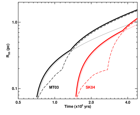
where is the initial electron density and is the radiative recombination coefficient of H+ to all levels with 2. We then assume that one of two processes occurs: either the Hii-region undergoes pressure-driven expansion; or that the Hii-region grows in size at constant density due to the increase in Lyman flux from the accreting star, followed by pressure-driven expansion once the star reaches fin. We then determine which of these results in the largest Hii-region. The differences between these two processes, in terms of the size evolution of the Hii-region, is illustrated in Fig. 4.
For pressure driven expansion of an Hii-region (see e.g. Dyson & Williams, 1997),
| (17) | |||||
| (18) |
with the Strömgren radius at ; the sound crossing time of the Strömgren sphere at ; the electron density at (assumed to be cm-3), and the sound speed in the gas (assumed to be 10 km s-1).
We then determine the radio flux at a given frequency of the Hii-region,
| (19) |
where is the Planck function, we assume a typical Hii-region temperature of 8000K (e.g. Dyson & Williams, 1997), and is the optical depth at frequency ,
| (20) | |||||

2.3.5 Source classification
Once the observable quantities of each source in the simulation have been computed, we first apply the detection limits of the RMS survey to determine whether or not they would form part of the RMS sample. As the initial source selection was done using MSX point-source fluxes, the first detection limit to apply is that of the MSX Galactic Plane survey at 21m. As the completeness limits of the MSX survey are not particularly well defined, we ran our own completeness tests using sample images from the survey data to calculate the detection limits as a function of Galactic position. These completeness tests and their results are described in more detail in Appendix B. For each source we compare the 21µm luminosity to the completeness as a function of 21µm flux at the source’s location on the sky, to determine the probability that the source would be detected. A random number is then generated, and the source is deemed to be detectable if .
Detected sources are classified as either YSOs or Hii-regions based on their calculated continuum radio fluxes and angular sizes. Again, we must then compare these fluxes to the detection limits of the multiple radio surveys that were used in the compilation of the RMS survey. If a source is determined to have a radio surface brightness in excess of the 3-limit along that line-of-sight, it is classified as a Hii-region. If the size of an object’s Hii-region is greater than the spatial resolution of the imaging part of the RMS survey (2′′), it is assumed that it would be resolved and therefore again classified as a Hii-region. If it is greater than the MSX beam size (20′′), it is assumed that the object would not belong to the MSX point-source catalogue, and so is discarded from the simulation. Objects which are not detected in the radio, are point-sources in the high-resolution RMS imaging, and are deemed to be detectable in the MSX survey, are classified as YSOs. The classification process is illustrated by the flow-chart in Fig. 5.
3 Results
In the following sections, we will describe the output of the model with various input parameters. Firstly, we concentrate on the results when the ‘fiducial’ set of input values are used.
| Parameter | Value |
|---|---|
| Accretion law | McKee & Tan (2003) |
| 1.0 g cm-2 | |
| 104cm-3 | |
| Gas distribution | Spiral arms only |
| IMF | Kroupa (2001) |
| SFRGal | 3⊙yr-1 |
3.1 Fiducial model
To first test the output of the model we start with a simulation for which the main parameters are set to fiducial values. These values are listed in Table 2.
For this initial model we start with the accretion law of MT03, with the parameter set to 1.0 g cm-2. In accord with the results of MT03, this implies that the mass at which massive stars join the MS, MS, is set to 20⊙. The initial electron density when the Hii region first turns on is set to 104cm-3, which is a typical value for ultra-compact Hii-regions (Wood & Churchwell, 1989). We use a Galactic gas distribution model in which star formation is confined to the spiral arms only (i.e. the ‘thin-disk’ and ‘thick-disk’ diffuse gas components are ignored). This is because, in the NE2001 model, the thin-disk component includes a dense circumnuclear ring of gas at a Galacto-centric distance of GC5kpc. This produces a large excess of sources at this location, which is not observed. The spiral arms on their own however reproduce the spatial distribution of sources reasonably well (see Sect. 3.2.2).
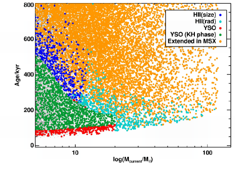
3.1.1 Illustration of classification criteria
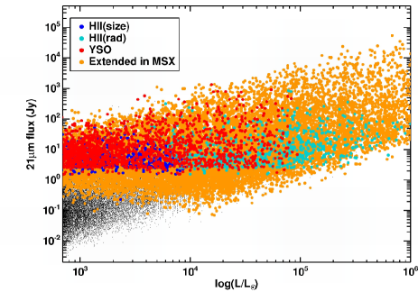
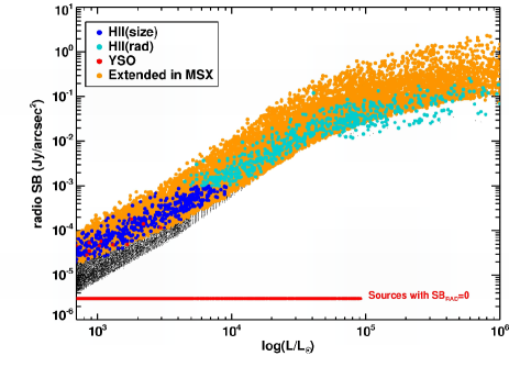
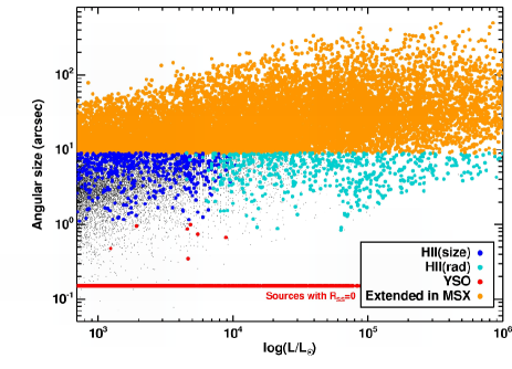
In Fig. 6 we illustrate the effect of our selection criteria on the output of the model. The top-left panel shows the 21m flux of each object, demonstrating that no sources below the MSX detection limit (4-10 Jy depending on location in the plane) are included in catalogue of young stars. The width and slope of the distribution of as a function of are governed by the empirically derived parameters of Eq. (14). Another feature of the simulation illustrated by this plot is the absence of YSOs above ⊙. This corresponds to the ZAMS luminosity of a star with ⋆= MS(=20⊙ in this simulation). That is, any star which has reached the MS and is ionizing its nebula is found to be detectable by the RMS radio observations.
In the top-right panel of Fig. 6 we plot the radio surface brightness of the objects in the simulation. The figure shows that only sources with surface brightnesses above 1 mJy/beam are detectable in the radio, and hence are classified as Hii regions from their radio emission. Below this limit there are further sources which are classified as Hii regions based on their angular size: an object which is radio-quiet, but that would be found to be extended in follow-up infrared imaging with spatial resolution 2′′ (i.e. has radius greater than 1′′), is also classified as a Hii region. This is shown again in the bottom-left panel of Fig. 6, we also illustrate the point at which evolved Hii regions are discarded from the simulation, i.e. when their angular sizes become larger than 18′′ and would no longer be point-sources in MSX. These ‘discarded’ stars are shown as yellow points.
Another aspect illustrated well by the top-right and bottom-left panels is that the observational and physical classification criteria match each other extremely well. Massive YSOs are defined physically as proto-stellar objects which have not yet contracted to their MS configuration, emit very little Lyman flux, and so are not surrounded by ionized gas. Meanwhile, the observational definition is of a proto-star which is bright in the mid-IR but that shows no evidence of a Hii-region, either from continuum radio emission of from spatially-extended mid-IR emission. In the top-right and bottom-left panels of Fig. 6 we see that there are very few objects misclassified as YSOs because their Hii-regions are too small or weak to be detected.
3.1.2 Lifetimes
The current age of the objects in each phase as a function of current mass is shown in the bottom right panel of Fig. 6. The objects classified as YSOs in the simulation all have masses below 20⊙ (MS in this simulation). That is, as soon as a massive star reaches the main-sequence and begins to ionize its surroundings, it becomes immediately detectable in the RMS radio observations and hence is classified as a Hii-region.
The age distribution of YSOs is a function of current stellar mass. For objects in the simulation with cur20⊙the YSO ages span 1-3yrs. Some of these objects are those with high final masses which are actively accreting. However, most of these YSOs are objects which have finished accreting are still contracting to the MS from their ‘swollen’ phase (shown as green points).
Once arriving on the MS, most objects are then picked up as Hii-regions. That is, there are very few YSOs outside the ‘YSO envelope’ clearly defined in the bottom right panel of Fig. 6 by the green and red points (see also discussion in previous Section). Objects with masses below 10⊙ have very faint radio emission, but are still detected as Hii-regions as the angular size of the gas bubble they drive is larger than the spatial resolution of the RMS follow-up mid-IR imaging. The Hii-region phase itself spans around 105yrs for lower mass objects, while it is about an order of magnitude shorter for the most massive stars.
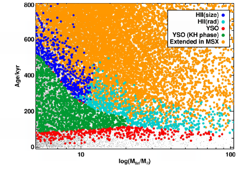
Another illustration of the phase lifetimes is plotted in Fig. 7. This plot demonstrates the time spent in each phase as a function of the final mass, fin. As stars initially grow in mass very slowly in the MT03 accretion rate model, no objects in the simulation become visible until around 40,000yrs. The YSO phase then lasts yrs for the lowest mass objects, a substantial fraction of which is spent contracting from the ‘swollen’ KH phase. For the most massive objects, which can reach the MS while still accreting, the YSO phase lasts yrs. Therefore, in these simulations, though the most massive YSOs are currently 20⊙, substantial numbers of these objects are still accreting and will go on to form stars well in excess of 20⊙.
3.2 Comparison to the RMS results
In the following sections we compare the results of our simulations to those of the RMS survey. The features that are readily comparable are the relative distributions of objects as a function of luminosity and Galactic position.
Within the RMS survey over 98% of the objects classified as being YSOs or Hii-regions now have unambiguous kinematic distances. To assess the impact of the remaining 2%, we compared three different observed luminosity distributions – one with the ambiguous distances set to the nearside distance, to the farside distance, and randomized between near and far. In practice we found that the differences between these three distributions were within the noise, and so have a negligible impact on our conclusions. When comparing with our simulated data, we adopted distances for these objects which were randomized between near and far.
3.2.1 Luminosity distribution
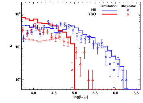
A powerful diagnostic of the RMS database is the relative numbers of YSOs and Hii-regions as a function of luminosity. The observational data are shown in Fig. 8 as data-points with error bars. It is clear that the observed distribution of YSOs peaks at a lower luminosity than does the Hii-region distribution, with many more Hii regions found at higher luminosities (see also Mottram et al., 2011b).
Overplotted in Fig. 8 are the results of our simulation with fidicial parameters. We first note that our fiducial model already provides qualitatively good fits to the data. The quantitative fit to the Hii-region data is also very good, while the simulated YSO distribution predicts numbers which are typically a factor of 2 too large. As will be shown later, by fine-tuning the model parameters we are able to provide excellent fits to the data.
The relative numbers of YSOs and Hii-regions (i.e. Hii) are also well matched. This is a validation of the approximations we made in calculating the observed properties of the Hii-regions. Under our current assumptions, almost every object in the simulation which has evolved as far as the MS is detected as a Hii-region (see also discussion in Sect. 3.1.1). If our assumptions underestimated the radio flux then the numbers YSOs/Hii-regions would be unchanged, as nearly all MS objects are already detected. Meanwhile, if we overestimated then the Hii-regions would still be picked up as being spatially extended (see top-right panel of Fig. 6). The physical sizes of the Hii-regions are goverened by their expansion rates, which in turn is dictated by the parameter . This can greatly alter the numbers of Hii-regions in the simulation while leaving the numbers of YSOs unchanged. Using the typical ultra-compact Hii-region value of =104cm-3 (Wood & Churchwell, 1989) we find excellent agreement between the simulated luminosity distributions of YSOs/Hii-regions and the RMS results.
One obvious feature of the simulated data is the steep drop-off in YSOs at ⊙, whereas the observations show a smoother drop-off at high luminosities. The location of this drop-off corresponds to the luminosity of objects with large fin when they arrive on the MS at MS. The parameter MS depends on the accretion rate – higher accretion rates mean that stars join the MS at higher masses. Therefore, we can adjust the location of the high-⋆ dropout by changing MS, or equivalently the accretion rate.
Finally, we address the topic of the pre-MS ‘swollen’ phase of massive stars. In Fig. 8, the solid and dotted lines show the luminosity distributions of simulations with and without a KH contraction phase respectively. As we have already illustrated in Figs. 6 and 7 the inclusion of a KH phase significantly prolongs the YSO phase in lower mass objects, and results in larger numbers of low-⋆ YSOs. In Fig. 8, we see that if we disregard the KH phase the number of low-⋆ YSOs is reduced. Meanwhile, the number of high-⋆ YSOs remains approximately the same, since any KH phase for these objects would be short compared to the age of the star when accretion terminates. The numbers of Hii-regions remain unchanged, since in our simulation the duration of the Hii phase is the same whether or not it is proceeded by a KH phase. These effects result in a poorer qualitative fit to the data compared to a simulation which includes a KH phase. We therefore conclude that a KH swollen phase is required for stars with masses 20⊙in order for our simulations to provide a good match to the data.

3.2.2 Galactic distribution
Another diagnostic of the RMS sample is the distribution of sources with Galactic position. As well as comparing with the source distribution in Galactic longitude and latitude , the radial velocity of each RMS source gives us an unambiguous measurement of Galacto-centric distance GC, assuming that the sources follow the Galactic rotation curve to within a few km s-1.
We again state that in our fiducial model we consider the star formation to follow the gas distribution in the spiral arms only. When including the full gas distribution model, which has components due to the thick disk as well as a ring of gas in the thin disk at GC5kpc, we found an extremely large overdensity of sources at low GC which is not seen in the data. Our results suggest that massive star formation is confined to the spiral arm component of the Galaxy.
The total distribution of YSOs and young Hii regions from the RMS survey with Galactic position and comparisons with the model results are shown in Fig. 9. As with the luminosity distributions in the previous section, the approximate normalization and overall trends of the simulations match the data rather well. However, there are qualitative features of the simulation which are not matched by the observed data. Firstly, there are two ‘horns’ in the number counts of the model’s -distribution, at ° and °. Secondly, in the -distribution the fall-off in source counts as one moves away from the plane is steeper in the observations than in the simulation. Thirdly, the right-hand panel of Fig. 9 shows that there is a surplus of sources in the simulation at GC8kpc with respect to the data.
These three features can all be understood as being due to the same feature in the Galactic gas distribution model. The horns in the -distribution are due to an overdensity of sources in the Sagittarius-Carina arm. As this arm passes close to the Sun, this also causes the overdensities of sources at high Galactic latitudes and at GC8kpc. In principle the RMS results could be used to fine-tune the description of the Galaxy’s gas content, however this is not the goal of the current work and we leave such a study for a future paper.
3.3 Effect of varying fiducial parameters
3.3.1 Stellar IMF and SFRGal
Broadly speaking, these parameters control the overall normalization of the predicted number of objects in the RMS survey. The IMF of Kroupa (2001) puts a significant amount of mass into objects with sub-Solar masses. If this were to be changed to another description of the IMF, such as a standard Salpeter law down to 0.8⊙, this would increase the number of massive objects in the simulation, though the relative numbers of objects as a function of mass would be unchanged. Though there is speculation as to variations in the slope of the IMF at high masses and to the presence of an upper-mass cutoff (Bastian et al., 2010), the numbers of objects in the RMS survey with inferred high masses (i.e. those with bol ⊙) are too few for us to test this.
The parameter SFRGal linearly affects the overall normalization, for example doubling SFRGal results in twice as many objects in the simulation. Changing the IMF to a Salpeter IMF would result in more massive stars, which would then require SFRGal to be decreased to maintain the same overall number counts of objects. However, the majority of independent estimates of SFRGal are above 2⊙yr-1, so there would be little justification in reducing this parameter beyond this value. The consistency in overall numbers between our simulations and the observations serve to justify our initial choices in SFRGal and the shape of the IMF. However, later in this study we will allow some variation in SFRGal in order to fine-tune the overall normalization.
3.3.2 Initial Hii region density
As has already been discussed, changes to this parameter affect only the duration of the Hii region phase. Increasing by a factor of ten from the fiducial value (i.e. to =105cm-3) causes the Hii regions to be initially more compact, and expand at a slower rate. As a result, the number of Hii regions in the this model is increased by a factor of 5 above those of the fiducial model. Similarly, dropping the density to =103cm-3 causes the Hii regions to rapidly expand once switched on, shortening the phase dramatically, leading to an under-prediction of the number of Hii regions again by a factor of 5. The fiducial value of =104cm-3 gives a good fit to the observed Hii-region distribution across all luminosities.
We note that, in reality, Hii-regions are likely to be expanding into a density gradient, leading to cometary morpholgies with size evolutions that differ from those calculated here (Arthur & Hoare, 2006). Our use of a constant simply represents an average over the early stages of a Hii-region’s evolution.
3.3.3 Stellar mass – QLyc relation
As discussed in Sect. 2.3.3, the relationship between stellar mass and the ionizing flux Lyc is uncertain. As has already been noted by Martins et al. (2005) the uncertainty in Lyc for a star of a given mass could be in excess of 50%, though we find from comparisons of various authors’ estimates of the mass – spectral-type relation that the uncertainty in Lyc for a given spectral-type may be as high as 0.7dex, or roughly a factor of five.
To investigate the effect of this uncertainty, two further simulations were run with Lyc scaled by 0.7dex. With Lyc decreased, Hii regions emit less radio flux and expand at a slower rate, meaning that the Hii region phase is prolonged. However, the vast majority of Hii regions are still picked up by the selection criteria, meaning that very few Hii regions are classified as YSOs in the simulation. The primary effect of decreasing Lyc is therefore to increase the number of Hii regions, though only by a factor of 2 in most luminosity bins.
Similarly, increasing Lyc by 0.7dex has only a mild impact on the results. The overall number of Hii regions is lowered due to the shorter Hii region lifetime, though again only by a factor of 2. So, despite the large uncertainty in the Lyc-cur relation, we conclude that this uncertainty has negligible impact on the results of our simulations.
4 Discussion: a comparison of different accretion laws
Thus far, all our models have used the MT03 prescription of accretion, in which cur, i.e. accretion which accelerates with time. In the following sections we investigate the free parameters in this prescription, as well as test other modes of accretion.
We measure how well a certain accretion law fits the data from the YSO bol-distribution only. This is because of (a) the large number of assumptions that have gone in to predicting the Hii-region properties, and (b) the morphology and normalization of the Hii-region bol-distribution can be augmented by altering parameters such as and Lyc, which are uncertain to factors of five. For now, we consider it a success of our model that the Hii-region bol-distribution is matched very well for the fiducial parameter values.
To assess the results produced by different accretion laws we employ a standard reduced- analysis between the observed and simulated bol-distributions. We have adaptively rebinned the observed YSO distribution such that there is a minimum of 9 objects per bin, i.e. that each bin has a minimum fractional error of 33% and therefore has a minimum significance of 3 in Poissonian statistics. For the simulated data we re-ran each simulation 50 times to reduce random errors to well below those of the observations.
We allowed the precise normalization of the bol-distribution to vary, since the parameter that affects overall numbers of objects (i.e. SFRGal) is itself uncertain, and we would not wish to discriminate against a particular accretion law simply because of a small offset in numbers. However, where a large normalization factor was required to achieve a minimal we critically assess the implications for the associated re-scaling of SFRGal. The best-fitting and associated SFRGal values for each model run are summarized in Table 3.
| Model & Parameter | SFRGal | |
|---|---|---|
| MT03 | ||
| = 0.1 g cm2 | 3.1 | 0.5 |
| = 1.0 g cm2 | 1.2 | 1.6 |
| = 10.0 g cm2 | 1.3 | 2.1 |
| B-H | ||
| MS= 15 ⊙ | 2.3 | 5.5 |
| MS= 20 ⊙ | 1.0 | 2.0 |
| MS= 30 ⊙ | 4.0 | 1.8 |
| Constant | ||
| form= 70 yrs | 3.6 | 1.6 |
| form= 300 yrs | 2.4 | 0.5 |
| form= 700 yrs | 0.7 | 0.6 |
| Uniform | ||
| = -3 | 41.2 | 7.7 |
| = -3.5 | 4.2 | 1.5 |
| = -4 | 92.6 | 3.1 |
| SK04 | ||
| MS= 15 ⊙ | 2.0 | 1.5 |
| MS= 20 ⊙ | 2.1 | 1.2 |
| MS= 25 ⊙ | 2.8 | 1.1 |
4.1 MT03 accretion
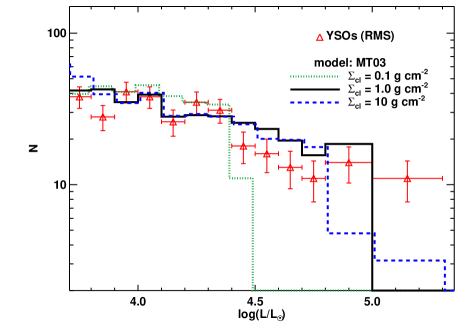
In the MT03 turbulent core model, the accretion rate of a star of a given final mass is dictated by the clump pressure and pressure structure. In their fiducial model this is parameterized in terms of the clump’s surface density . Increasing the accretion rate not only leads to faster formation times, but also results in high fin stars joining the MS at higher masses (i.e. MS increases, due to greater ‘swelling’ in the accretion phase). According to MT03, varying between 0.1 and 10g cm-2 results in values of MS between 12 and 24⊙. In Fig. 10 we show luminosity distributions using the extrema for these values of and MS.
The low- model has large differences to the fiducial model. The decreased accretion rates have the effect of lengthening the YSO phase, which is now dominated by stars still accreting rather than by stars which have finished accreting and are contracting to the MS. This means that the total number of low luminosity YSOs in the simulation is much larger, and to match the observed YSO levels in Fig. 10 we had to normalize the data by reducing the numbers of objects by a factor of 6. The only physical explanation for this normalization factor would be to reduce the Galactic star formation rate to SFRGal0.5⊙yr-1, whereas the vast majority of estimates of this quantity are 2⊙yr-1(see Diehl et al., 2006, and refs therein). Also, the decrease in MS pushes the YSO drop-out to lower luminosities, making it much more pronounced, and in clear disagreement with the RMS results. This is reflected in the poorer value when compared to other model runs of this scenario.
The fiducial and high- models match the observations very well. The high- model has a higher value of MS than the fidicial model, the effect of which is to push the YSO drop-out to higher luminosities. As the steepness of the IMF dictates that there are fewer objects at these higher luminosities, this makes the drop-out slightly less dramatic. The faster accretion rates mean that massive stars form quicker, however this does not greatly affect the distributions of YSOs. The YSO population is dominated by those objects with finMS, and a substantial fraction of the YSO lifetime of these objects is the Kelvin-Helmholz contraction phase, which is independent of the accretion rate in our model. The objects with finMS spend very little time in the YSO phase in the fiducial model (cf. Fig. 7), so decreasing the contribution of such objects to the YSO population does little to the observed YSO distribution, as the high fin stars spend most of their formative years as Hii regions.
In terms of which value of produces the best fit, the fiducial model achieves the lowest reduced : the =1g cm-2 model has =1.2, and the =10g cm-2 has =1.4. Given the similarity of these values, and the random uncertainty associated with how the data are binned, we consider each of these models to produce equally good fits. However, the fiducial value of is comparable to that typically observed in Galactic star-forming clumps (Plume et al., 1997), whereas a value of =10g cm-2 seems excessively high and is not supported by observations. The renormalization factor for the =1g cm-2 model is 0.65, implying a global star formation rate of SFRGal=1.6⊙yr-1. This is reasonably consistent with the vast majority of estimates of this parameter, which place it in the range 2-4⊙yr-1. Therefore, we consider that the =1g cm-2 model provides a good match to the data while being consistent with complimentary observations of star-forming clumps.
4.2 Bondi-Hoyle accretion
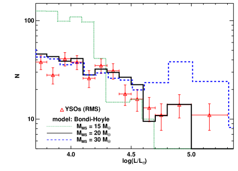
The simple Bondi-Hoyle (BH) ‘competitive’ accretion model we are using has the attractive property that it has very few free parameters once we employ the normalization of Bonnell & Bate (2006). We are not aware of any robust numerical simulations of BH accretion which predict properties such as MS and MS contraction time, so in these simulations we have assumed that the MS contraction time approximates to the Kelvin-Helmholz time, in accord with the results of HO09. We allow MS to remain a free parameter, and explore the range MS=15-30⊙ which are typical values taken from the other accretion laws studied here. In Fig. 11 we show the results of these simulations with three different values of MS between 15 and 30⊙. The qualitative agreement with the RMS data is very good when MS is between 20-30⊙, while the overall normalization is also very good: optimal renormalization factors were found of 0.6, implying SFRGal between 1.7-2.0⊙yr-1.
The best fitting model is that with MS=20⊙, with reduced =1.0. This value of MS seems reasonable, given the quantitative results of MT03 and HO09 who find MS=12-30⊙ depending on the accretion history of the protostar. The optimal normalization of this model requires SFRGal=1.9⊙yr-1, which again is reasonable given other measurements of this value.
4.3 Constant accretion
In this section we explore two distinct scenarios. Firstly, we investigate a uniform accretion rate for all stars, regardless of mass. Secondly, we fix the accretion rate such that fin/ is constant, that is that all stars finish accreting on the same timescale form, independent of fin.
4.3.1 Uniform
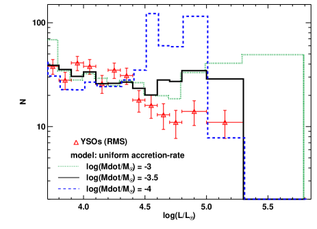
The luminosity distributions for three values of are shown in Fig. 12 using the computed tracks at =10-3⊙yr-1 and 10-4⊙yr-1, and a track linearly interpolated between these two at 10-3.5⊙yr-1. For each track we found the value of MS by plotting the track on a H-R diagram and finding the approximate mass at which the track joined the ZAMS of (Meynet & Maeder, 2000). The value of MS was 27⊙ for the and ⊙yr-1 tracks, and 36⊙ for the ⊙yr-1 track.
While the normalization is reasonable (see Table 3 for the implied values of SFRGal), these models give poor qualitative fits to the data. The reason for this is that in the HO09 accretion tracks, the behaviour of bol with cur is such that at some point bol reaches a temporary plateau. In the simulation, this causes a pile-up of objects at a certain luminosity. For example, in the =10-4⊙yr-1 this plateau occurs at bol⊙, leading to a spike in the luminosity distribution at this value (see the blue dashed curve in Fig. 12). Similarly, in the =10-3⊙yr-1 model, this pile-up occurs at bol⊙. The interpolated model (=10-3.5⊙yr-1) does not have any such pronounced spikes in the luminosity distribution as the interpolation process serves to smooth any such spikes out. However, this model still produces a poor qualitative fit to the data, the bol-distribution being significantly flatter than the observations.
4.3.2 Uniform form
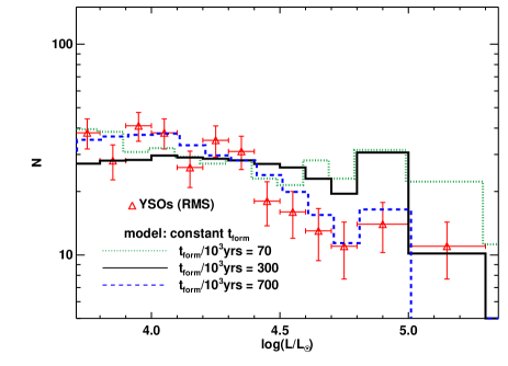
Here, we experiment with using accretion rates which are constant with time, but depend on the final mass of the star in such a way that all stars accrete their matter on identical timescales. To do this, we took the birthlines of HO09, which are sampled at accretion rates of 10-5, 10-4 and 10-3⊙yr-1 and linearly interpolated them onto a finer grid, sampling at every 0.01dex. For each star in the simulation we then calculated the accretion rate required for it to form in a time form, where form is a free parameter, and assigned each star a constant accretion rate of =fin/form. The lowest values of were clipped at 10-5⊙yr-1, and the highest at 10-3⊙yr-1, as we have no birthline calculations outside this range.
The point at which each star joins the MS, MS, is then a function of the star’s final mass. To determine MS as a function of we plotted each interpolated track on a H-R diagram and identified the approximate point at which it joined the ZAMS track of (Meynet & Maeder, 2000). Stars with finMS were again assumed to undergo a contraction phase before arriving on the MS, with the length of this phase equal to the K-H timescale of a star of that mass.
We can summarize the predicted behaviour of such models as follows. The effect of decreasing form is to increase the accretion rates. This means that stars can pass through the YSO phase more quickly, resulting in less YSOs in each luminosity bin. However, this effect is mitigated by the fact that the higher accretion rates push the value of MS to higher masses, extending the length of the YSO phase for objects with high fin. Altering form can therefore affect both the qualitative shape and the overall normalization of the bol-distribution.
The results of simulations with three different values of uniform form are shown in Fig. 13. As expected, in the simulation with short formation timescales (form=yrs) the YSOs have higher luminosities than in the simulations with longer form. The large value of MS (40⊙) means that the numbers of YSOs with bol⊙ are overpredicted by factors of 2-3 compared with the lower luminosity objects. At longer formation timescales of form=yrs the YSO drop-out matches the observations slightly better, though the simulated distribution is again ‘top-heavy’ compared to the observations. The simulation with the longest form produces a very good qualitative fit to the data. However, the predicted numbers of YSOs are too large by a factor of five, requiring SFRGal to be reduced to 0.6⊙yr-1 to match the observed levels.
4.4 Decelerating accretion
As already discussed in Sect. 4, the prescription of decelerating accretion from Schmeja & Klessen (2004) cannot produce massive stars within a reasonable formation timescale when using the standard values for the constants in Eq. (11). Massive stars can be formed however if the constants are pushed to the boundaries of their uncertainties. This maximises the value of in Eq. (13), and allows the protostars to spend more time at high accretion rates. For the analysis in this Section, we use values of yrs and yrs.
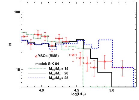
Figure 14 shows the luminosity distribution of young massive stars from the simulation using the decelerating accretion model. The SK04 accretion model provides no estimate of MS, but the low accretion rates as the star is approaching its final mass suggest that MS may be lower under this model than for the constant and accelerating models. In Fig. 14 we show simulation results for three different values of MS.
The qualitative shape of the YSO bol-distribution this time does not match the observations. The longer time that YSOs spend at higher masses compared to the accelerating accretion models produces a luminosity distribution which is more top-heavy than the observations. This is reflected in the values, which are higher than those of the accelerating accretion models.
The overall numbers of objects, as with the constant rate accretion law, are overpredicted in this model – to achieve the correct normalization each histogram had to be scaled down by factors of 2-3, implying global star-formation rates below 1-1.5⊙yr-1. Meanwhile, the qualitative shape of the models’ bol-distributions is much flatter than the observations. This is due to the very high accretion rates that objects have at early times, and hence higher accretion luminosities. The net effect is that lower mass objects are moved to higher luminosity bins with respect to accelerating accretion models, producing a flatter bol-distribution.
4.5 Which accretion laws fit the data best?
We now discuss which of the accretion models we have tested best fits the observed luminosity distribution of the RMS survey data, taking into account the results described in this section thus far.
The first conclusion that we draw is that the decelerating accretion scenario is the least likely of all those studied here. While it may be argued that the prescription of SK04 is only calibrated between 1-10⊙, the poor match between the data and the observations is still evident at low luminosities (and hence at masses between 5 and 20⊙). Also, irrespective of the prescription’s quantitative details, the qualititave effect of a decelerating accretion law is to produce a flat luminosity distribution of YSOs. Therefore, we conclude that this mechanism is unlikely to be the prevalent mode of massive star formation in our Galaxy. There are however caveats to this statement as we made several approximations in our calculations, such as that of the accretion luminosity of massive protostars, and of objects joining the MS mid-way through their accretion phase just as the accelerating accretion models do. Stronger critical analysis of the decelerating accretion scenario awaits the numerical predictions of the accretion luminosities and pre-MS tracks of massive stars forming in this way.
Similarly, we also argue against the uniform accretion rate models. Models where all stars accrete at exactly the same rate produce spikes in the luminosity distribution due to the discrete features in the HO09 accretion tracks, while the global gradients of the simulated bol-distributions are much flatter than that observed.
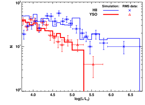
The uniform form models do produce very good qualitative fits to the data, but only if the formation timescale is very long, i.e. yrs. As previously discussed, using the fiducial value of SFRGal this produces greater numbers of YSOs than are observed. To recover the observed numbers, it requires that SFRGal be reduced to 0.6⊙yr-1, a factor of five lower than the typically-quoted value of 3⊙yr-1, and below even the lower limit of Robitaille & Whitney (2010), whose estimate of SFRGal is significantly lower than any other recent measurements. Further, this formation timescale would imply accretion-rates for massive stars of ⊙yr-1, which are an order of magnitude lower than current observational and theoretical estimates (e.g. Krumholz et al., 2009; Qiu et al., 2011).
The best fits are produced by the two accelerating accretion models. Both produce reduced statistics close to unity (see Table 3), and hence provide excellent fits to the data given the experimental uncertainties. At the same time, the number of sources in each model is a close match to the observations, meaning that the implied SFRGal remains sensible: we find best fitting average Galactic star-formation rates of 1.6⊙yr-1 and 2.0⊙yr-1 for the MT03 and BH models respectively. These are consistent with most recent measurements of this property (see Diehl et al., 2006; Robitaille & Whitney, 2010, and references therein).
At this stage, we are unable to conclusively state which of the accelerating models fits the data best. Random errors in, for example, how the data are binned, mean that the difference in the statistic between the two models is not significant. We should state that the MT03 model has a more rigorous quantitative basis compared to our BH model, which simply assumes the analytical formula for Bondi-Hoyle accretion and ad-hoc estimates for MS. Thorough numerical calculations of each scenario may in future allow us to distinguish decisively between the two.
In Fig. 15 we plot the YSO and Hii-region luminosity distributions for the best-fit model. We have chosen the BH model, since this gives a slightly lower than the MT03 model, and we have increased MS to 23⊙ to match the largest YSO luminosity bin, though this is more for aesthetic purposes since the reduced is no better than for MS=20⊙. Since the overall level of Hii-regions was slightly underpredicted, we have increased the initial electron density to = to slightly prolong the Hii-region phase and therefore increase the overall number of objects. Note that this value of is consistent with the typically quoted densities for ultra-compact Hii-regions of (Wood & Churchwell, 1989).
We can highlight two features of Fig. 15 where there is room for improvement in the fit. Firstly, the simulated YSO cutoff occurs at lower luminosities than in the observed trend. A better fit may be obtained by using values of MS which depend on fin rather than a single blanket value. Since MS depends on accretion history (see HO09, plus discussion in this work), which in turn depends on stellar mass in the accelerating accretion rate models, it is entirely plausible that MS may be dependent on final stellar mass. This would then serve to smooth-out the YSO cutoff and make it more like the observations.
Secondly, there is an apparent downturn in the Hii-region luminosity distribution at low luminosities, which is not reproduced in our simulations. An improvement to the fit may be obtained if lower fin objects have lower initial gas densities once they have reached the MS. Since low density regions expand at a faster rate, this will cause the Hii-region phase lifetime to be shorter for these objects. Though there are a large number of assumptions that go into our simulation of the Hii-region distribution, it is not an unreasonable expectation that higher mass stars should form in regions of higher gas densities.
4.6 Phase lifetimes of the best-fit model
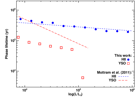
For our best-fitting model described in the previous Section, we now revisit the topic of the YSO and Hii-region phase lifetimes. For this, we compare to our recent empirical estimates presented in Mottram et al. (2011a). In that study, the lifetimes were estimated by dividing the number of objects per luminosity bin by the number of OB stars with the same luminosity, then multiplying by the MS lifetime of OB stars. There are three main sources of uncertainty in estimating phase lifetimes in this way. Firstly, the OB star population of the Galaxy is only complete within a few kiloparsecs of the Sun, which serves to increase the random errors. Secondly, the relationship between spectral type, stellar luminosity and stellar mass is still uncertain, and may introduce systematic errors, though we mitigate this uncertainty by using the same sources for these relations. Finally, this method gives phase lifetime as a function of luminosity, which for actively accreting objects is variable throughout their formation. However, our simulation provides a ‘snap-shot’ of the Galaxy’s population of young massive stars in a way designed to mimic the RMS survey. Therefore, we can make a quantitative measurement of lifetime versus bol from our simulation, despite the fact that objects may migrate from bin to bin throughout their evolution.
To calculate the lifetime as a function of luminosity, we first construct a diagnostic diagram of the simulation similar to that of the lower-left panel in Fig. 6, but plotting age against bol. Then, for a given luminosity bin, we determine the age range (i.e. the difference between the minimum to maximum ages) of all YSOs/Hii-regions in that bin, discarding the oldest and youngest 5% of objects to limit the impact of statistical outliers. The results of this analysis are plotted in Fig. 16, where we also compare with the results of Mottram et al. (2011a) which are illustrated by the long- and short-dashed lines.
We find that the lifetimes of YSOs are typically yrs with shorter lifetimes for the more luminous objects, predominantly an effect of the reduction in KH timescales at higher masses. On the other hand, Hii-region lifetimes show a weaker dependence on luminosity, spanning a factor of 3 between across the plotted luminosity range333Note that this lifetime refers to that of compact phase of the Hii-region, such that it would be detected in the RMS survey. . This can easily be understood from a numerical analysis of Eqs. (16) and (18) and the Lyman fluxes from Table 1 (see Sect. 2.3.4), which show that the expansion rates of Hii-regions span a similar factor of 3 across the range of luminosities plotted in Fig. 16, under the assumption of initial gas densities which are uniform across all objects.
The agreement between the two estimates of Hii-region lifetimes is excellent. Recall that we have already fine-tuned the initial electron density in order to match the observed numbers of Hii-regions. Since the observed number of objects at any given time is a product of the production rate and the lifetime, the fact that we can match the lifetimes and overall numbers simultaneously must mean that we also have an accurate estimate of the production rate (i.e. the globally averaged star-formation rate). In other words, the overall number of Hii-regions depends on SFRGal and , whereas the lifetime depends on only .
In terms of the YSOs, there is an apparent discrepancy between the two estimates. The systematic errors quoted by Mottram et al. (2011a), 0.45dex in the zero-point and 0.5 in the gradient, mean that the differences are significant only at the 1-2 level. In addition, the differences in gradient can in part be explained by the way in which Mottram et al. (2011a) determined the YSO lifetimes. As discussed above, these authors assumed a 1:1 correspondance between the luminosities of the YSOs and the those of main-sequence (MS) stars. However, since YSOs are often accreting objects they will have some accretion luminosity, and so their total luminosities will exceed those of MS stars with the same mass. In contrast, the majority of Hii-regions in our simulation have finished accreting, and have bolometric luminosities comparable to their MS luminosities.
For the simulation used in Fig. 16, we found that if the YSOs bolometric luminosities were used to estimate cur (i.e from interpolation of Table 1), then the current masses were typically overestimated by around 30%. This leads to the ratio of the number of YSOs to the number of MS stars at a given mass being over-predicted, and ultimately to overestimates of the YSO lifetimes. Quantitatively, we find that this overestimate in lifetimes is 70% at bol=⊙, and 40% at bol=⊙. Though this effect is not large enough to fully explain the discrepancy in YSO lifetimes in Fig. 16, it may be a contributing factor to the difference between the two gradients.
5 Summary
We have constructed a model to simulate the distributions and physical properties of massive protostars throughout the Galaxy, with the aim of predicting the observed luminosity distribution of massive Young Stellar Objects (YSOs) from the RMS survey. To compute the observed properties of each protostar in the simulation we employed several different prescriptions of the rates at which stars accrete mass as a function of time. For each accretion model we identified the parameters which produced the best qualitative fit to the observed YSO bol-distribution, allowing the global star formation rate SFRGal to vary to optimize the overall normalization.
Our main findings may be summarized as follows:
-
•
The luminosity distribution of YSOs is best described using accretion rates which increase as the star grows in mass. Accretion rates which were constant in time or which decreased as the star grew in mass were ruled out, as they either produced poor qualitative fits, produced far too many YSOs, or both.
-
•
The lack of YSOs at high luminosities is consistent with a picture of star-formation whereby stars arrive on the main-sequence (MS) once they reach a mass of 20-30⊙, even if the final mass of the star is well in excess of this value. We suggest that the precise mass at which stars arrive on the MS may be some function of the final stellar mass.
-
•
In order to produce a satisfactory qualitative fit to the YSO distribution at low luminosities, an intermediate radio-quiet phase is required between the end of accretion and the ignition of a Hii-region. The length of this phase is well described by the star’s Kelvin-Helmholz timescale, and therefore is consistent with a ‘swollen star’ period of pre-MS evolution for stars with masses 5-20⊙.
-
•
The maximum final stellar mass fin at which stars no longer experience this ‘swollen’ phase is indicated by the observed drop-off in YSO numbers at ⊙. This corresponds to stars with masses fin20⊙, which in our simulations have accretion rates of 1-4 ⊙yr-1.
-
•
From the best-fit models we find that the overall numbers of objects can be well reproduced by a globally averaged star-formation rate of the Galaxy of 1.5-2⊙yr-1.
-
•
Our best-fit model predicts phase lifetimes for YSOs of yrs, falling off dramatically for objects with bol⊙. The compact Hii-regions in the RMS survey have phase lifetimes between 2-4yrs.
In the future, the framework of the simulations presented here could be adapted to investigate Galactic structure, once the distances to the RMS survey objects are known to a greater precision. Future modelling of the RMS population will take into account the evolution of the SED. This will include the increasing luminosity and heating as well as the dispersal of circumstellar material by feedback. Bipolar cavities in particular make the SED dependent on the viewing angle (Whitney et al., 2003) and a simulation of a large sample with random viewing angles will be constrained by comparison with the colour distribution as well as properties of the CO outflows and near-IR reflection nebulae.
Acknowledgments
We thank Jonathan Tan and Willem-Jan de Wit for many useful discussions during the course of this work. BD is funded by a fellowship from the Royal Astronomical Society.
References
- Arthur & Hoare (2006) Arthur, S. J. & Hoare, M. G. 2006, ApJS, 165, 283
- Ascenso et al. (2007) Ascenso, J., Alves, J., Vicente, S., & Lago, M. T. V. T. 2007, A&A, 476, 199
- Bastian et al. (2010) Bastian, N., Covey, K. R., & Meyer, M. R. 2010, ARA&A, 48, 339
- Benjamin et al. (2005) Benjamin, R. A., Churchwell, E., Babler, B. L., Indebetouw, R., Meade, M. R., Whitney, B. A., Watson, C., Wolfire, M. G., Wolff, M. J., Ignace, R., Bania, T. M., Bracker, S., Clemens, D. P., Chomiuk, L., Cohen, M., Dickey, J. M., Jackson, J. M., Kobulnicky, H. A., Mercer, E. P., Mathis, J. S., Stolovy, S. R., & Uzpen, B. 2005, ApJ, 630, L149
- Berdnikov et al. (2000) Berdnikov, L. N., Dambis, A. K., & Vozyakova, O. V. 2000, A&AS, 143, 211
- Bernasconi & Maeder (1996) Bernasconi, P. A. & Maeder, A. 1996, A&A, 307, 829
- Bibby et al. (2008) Bibby, J. L., Crowther, P. A., Furness, J. P., & Clark, J. S. 2008, MNRAS, 386, L23
- Blanc et al. (2009) Blanc, G. A., Heiderman, A., Gebhardt, K., Evans, N. J., & Adams, J. 2009, ApJ, 704, 842
- Bonnell & Bate (2006) Bonnell, I. A. & Bate, M. R. 2006, MNRAS, 370, 488
- Brandner et al. (2008) Brandner, W., Clark, J. S., Stolte, A., Waters, R., Negueruela, I., & Goodwin, S. P. 2008, A&A, 478, 137
- Chapman et al. (2009) Chapman, N. L., Mundy, L. G., Lai, S.-P., & Evans, N. J. 2009, ApJ, 690, 496
- Cordes & Lazio (2002) Cordes, J. M. & Lazio, T. J. W. 2002, ArXiv Astrophysics e-prints
- Davies et al. (2009) Davies, B., Figer, D. F., Kudritzki, R., Trombley, C., Kouveliotou, C., & Wachter, S. 2009, ApJ, 707, 844
- Davies et al. (2007) Davies, B., Figer, D. F., Kudritzki, R.-P., MacKenty, J., Najarro, F., & Herrero, A. 2007, ApJ, 671, 781
- Davies et al. (2008) Davies, B., Figer, D. F., Law, C. J., Kudritzki, R.-P., Najarro, F., Herrero, A., & MacKenty, J. W. 2008, ApJ, 676, 1016
- Diehl et al. (2006) Diehl, R., Halloin, H., Kretschmer, K., Lichti, G. G., Schönfelder, V., Strong, A. W., von Kienlin, A., Wang, W., Jean, P., Knödlseder, J., Roques, J., Weidenspointner, G., Schanne, S., Hartmann, D. H., Winkler, C., & Wunderer, C. 2006, Nature, 439, 45
- Diolaiti et al. (2000) Diolaiti, E., Bendinelli, O., Bonaccini, D., Close, L., Currie, D., & Parmeggiani, G. 2000, A&AS, 147, 335
- Draine (1989) Draine, B. T. 1989, in ESA Special Publication, Vol. 290, Infrared Spectroscopy in Astronomy, ed. E. Böhm-Vitense, 93–98
- Dyson & Williams (1997) Dyson, J. E. & Williams, D. A. 1997, The physics of the interstellar medium, ed. Dyson, J. E. & Williams, D. A.
- Egan et al. (2003) Egan, M. P., Price, S. D., Kraemer, K. E., Mizuno, D. R., Carey, S. J., Wright, C. O., Engelke, C. W., Cohen, M., & Gugliotti, M. G. 2003, VizieR Online Data Catalog, 5114, 0
- Ellingsen (2006) Ellingsen, S. P. 2006, ApJ, 638, 241
- Flaherty et al. (2007) Flaherty, K. M., Pipher, J. L., Megeath, S. T., Winston, E. M., Gutermuth, R. A., Muzerolle, J., Allen, L. E., & Fazio, G. G. 2007, ApJ, 663, 1069
- Foster & Chevalier (1993) Foster, P. N. & Chevalier, R. A. 1993, ApJ, 416, 303
- Froebrich et al. (2006) Froebrich, D., Schmeja, S., Smith, M. D., & Klessen, R. S. 2006, MNRAS, 368, 435
- Harayama et al. (2008) Harayama, Y., Eisenhauer, F., & Martins, F. 2008, ApJ, 675, 1319
- Hoare et al. (2005) Hoare, M. G., Lumsden, S. L., Oudmaijer, R. D., Urquhart, J. S., Busfield, A. L., Sheret, T. L., Clarke, A. J., Moore, T. J. T., Allsopp, J., Burton, M. G., Purcell, C. R., Jiang, Z., & Wang, M. 2005, in IAU Symposium, Vol. 227, Massive Star Birth: A Crossroads of Astrophysics, ed. R. Cesaroni, M. Felli, E. Churchwell, & M. Walmsley, 370–375
- Hosokawa & Omukai (2009) Hosokawa, T. & Omukai, K. 2009, ApJ, 691, 823
- Kahn (1974) Kahn, F. D. 1974, A&A, 37, 149
- Kennicutt (1998) Kennicutt, Jr., R. C. 1998, ApJ, 498, 541
- Kothes & Dougherty (2007) Kothes, R. & Dougherty, S. M. 2007, ArXiv e-prints, 0704.3073
- Kroupa (2001) Kroupa, P. 2001, MNRAS, 322, 231
- Krumholz et al. (2009) Krumholz, M. R., Klein, R. I., McKee, C. F., Offner, S. S. R., & Cunningham, A. J. 2009, Science, 323, 754
- Kuiper et al. (2011) Kuiper, R., Klahr, H., Beuther, H., & Henning, T. 2011, ApJ, 732, 20
- Kurtev et al. (2007) Kurtev, R., Borissova, J., Georgiev, L., Ortolani, S., & Ivanov, V. D. 2007, A&A, 475, 209
- Lanz & Hubeny (2007) Lanz, T. & Hubeny, I. 2007, ApJS, 169, 83
- Lumsden et al. (2002) Lumsden, S. L., Hoare, M. G., Oudmaijer, R. D., & Richards, D. 2002, MNRAS, 336, 621
- Lutz (1999) Lutz, D. 1999, in ESA Special Publication, Vol. 427, The Universe as Seen by ISO, ed. P. Cox & M. Kessler, 623–+
- Martins & Plez (2006) Martins, F. & Plez, B. 2006, A&A, 457, 637
- Martins et al. (2005) Martins, F., Schaerer, D., & Hillier, D. J. 2005, A&A, 436, 1049
- McKee & Tan (2003) McKee, C. F. & Tan, J. C. 2003, ApJ, 585, 850
- Melena et al. (2008) Melena, N. W., Massey, P., Morrell, N. I., & Zangari, A. M. 2008, AJ, 135, 878
- Messineo et al. (2009) Messineo, M., Davies, B., Ivanov, V. D., Figer, D. F., Schuller, F., Habing, H. J., Menten, K. M., & Petr-Gotzens, M. G. 2009, ApJ, 697, 701
- Messineo et al. (2008) Messineo, M., Figer, D. F., Davies, B., Rich, R. M., Valenti, E., & Kudritzki, R. P. 2008, ApJ, 683, L155
- Messineo et al. (2005) Messineo, M., Habing, H. J., Menten, K. M., Omont, A., Sjouwerman, L. O., & Bertoldi, F. 2005, A&A, 435, 575
- Meynet & Maeder (2000) Meynet, G. & Maeder, A. 2000, A&A, 361, 101
- Motoyama & Yoshida (2003) Motoyama, K. & Yoshida, T. 2003, MNRAS, 344, 461
- Mottram et al. (2011a) Mottram, J. C., Hoare, M. G., Davies, B., Lumsden, S. L., Oudmaijer, R. D., Urquhart, J. S., Moore, T. J. T., Cooper, H. D. B., & Stead, J. J. 2011a, ApJ, 730, L33+
- Mottram et al. (2007) Mottram, J. C., Hoare, M. G., Lumsden, S. L., Oudmaijer, R. D., Urquhart, J. S., Sheret, T. L., Clarke, A. J., & Allsopp, J. 2007, A&A, 476, 1019
- Mottram et al. (2011b) Mottram, J. C., Hoare, M. G., Urquhart, J. S., Lumsden, S. L., Oudmaijer, R. D., Robitaille, T. P., Moore, T. J. T., Davies, B., & Stead, J. 2011b, A&A, 525, A149+
- Plume et al. (1997) Plume, R., Jaffe, D. T., Evans, II, N. J., Martin-Pintado, J., & Gomez-Gonzalez, J. 1997, ApJ, 476, 730
- Qiu et al. (2011) Qiu, K., Zhang, Q., & Menten, K. M. 2011, ApJ, 728, 6
- Rathborne et al. (2010) Rathborne, J. M., Jackson, J. M., Chambers, E. T., Stojimirovic, I., Simon, R., Shipman, R., & Frieswijk, W. 2010, ApJ, 715, 310
- Reid et al. (2009) Reid, M. J., Menten, K. M., Zheng, X. W., Brunthaler, A., Moscadelli, L., Xu, Y., Zhang, B., Sato, M., Honma, M., Hirota, T., Hachisuka, K., Choi, Y. K., Moellenbrock, G. A., & Bartkiewicz, A. 2009, ApJ, 700, 137
- Robitaille & Whitney (2010) Robitaille, T. P. & Whitney, B. A. 2010, ApJ, 710, L11
- Robitaille et al. (2006) Robitaille, T. P., Whitney, B. A., Indebetouw, R., Wood, K., & Denzmore, P. 2006, ApJS, 167, 256
- Schaller et al. (1992) Schaller, G., Schaerer, D., Meynet, G., & Maeder, A. 1992, A&AS, 96, 269
- Schmeja & Klessen (2004) Schmeja, S. & Klessen, R. S. 2004, A&A, 419, 405
- Shu (1977) Shu, F. H. 1977, ApJ, 214, 488
- Stahler et al. (2000) Stahler, S. W., Palla, F., & Ho, P. T. P. 2000, Protostars and Planets IV, 327
- Tapia et al. (2003) Tapia, M., Roth, M., Vázquez, R. A., & Feinstein, A. 2003, MNRAS, 339, 44
- Taylor & Cordes (1993) Taylor, J. H. & Cordes, J. M. 1993, ApJ, 411, 674
- Urquhart et al. (2007a) Urquhart, J. S., Busfield, A. L., Hoare, M. G., Lumsden, S. L., Clarke, A. J., Moore, T. J. T., Mottram, J. C., & Oudmaijer, R. D. 2007a, A&A, 461, 11
- Urquhart et al. (2007b) Urquhart, J. S., Busfield, A. L., Hoare, M. G., Lumsden, S. L., Oudmaijer, R. D., Moore, T. J. T., Gibb, A. G., Purcell, C. R., Burton, M. G., & Marechal, L. J. L. 2007b, A&A, 474, 891
- Urquhart et al. (2008) Urquhart, J. S., Busfield, A. L., Hoare, M. G., Lumsden, S. L., Oudmaijer, R. D., Moore, T. J. T., Gibb, A. G., Purcell, C. R., Burton, M. G., Maréchal, L. J. L., Jiang, Z., & Wang, M. 2008, A&A, 487, 253
- Urquhart et al. (2009a) Urquhart, J. S., Hoare, M. G., Lumsden, S. L., Oudmaijer, R. D., Moore, T. J. T., Brook, P. R., Mottram, J. C., Davies, B., & Stead, J. J. 2009a, A&A, 507, 795
- Urquhart et al. (2009b) Urquhart, J. S., Hoare, M. G., Purcell, C. R., Lumsden, S. L., Oudmaijer, R. D., Moore, T. J. T., Busfield, A. L., Mottram, J. C., & Davies, B. 2009b, A&A, 501, 539
- Whitney et al. (2003) Whitney, B. A., Wood, K., Bjorkman, J. E., & Wolff, M. J. 2003, ApJ, 591, 1049
- Whitworth & Ward-Thompson (2001) Whitworth, A. P. & Ward-Thompson, D. 2001, ApJ, 547, 317
- Wolfire & Cassinelli (1987) Wolfire, M. G. & Cassinelli, J. P. 1987, ApJ, 319, 850
- Wood & Churchwell (1989) Wood, D. O. S. & Churchwell, E. 1989, ApJS, 69, 831
- Zinnecker & Yorke (2007) Zinnecker, H. & Yorke, H. W. 2007, ARA&A, 45, 481
Appendix A Computation of line-of-sight extinction
In calculating the extinction towards each object in our simulation, we cannot simply use 2-D extinction maps of the Galactic Plane, as these do not give any indication of how extinction varies with distance along a given sightline. Instead, we use test points with known distances and extinctions, and derive a relation between the intervening gas column density and the line of sight extinction by assuming that the extinction is some function of the interstellar gas column density between the Earth and the object. This relation should be linear, as they are both directly proportional to the optical depth.

| Name | (°) | (°) | D⊙(kpc) | Ak | Ref |
|---|---|---|---|---|---|
| 1806-20 | 10.00 | -0.24 | 8.7 | 3.00.3 | 1 |
| CL1813 | 12.77 | -0.01 | 4.70.4 | 0.830.2 | 2 |
| Quartet | 24.90 | +0.12 | 6.10.6 | 1.60.4 | 3 |
| RSGC1 | 25.27 | -0.16 | 6.60.9 | 2.600.07 | 4 |
| RSGC2 | 26.19 | -0.07 | 5.8 | 1.440.05 | 5 |
| 1900+14 | 43.02 | +0.77 | 12.51.7 | 1.380.06 | 6 |
| GLIMPSE20 | 44.16 | -0.07 | 4.50.7 | 1.20.2 | 3 |
| Tr14 | 287.40 | -0.58 | 2.70.3 | 0.290.05 | 7,8 |
| NGC3603 | 291.63 | -0.53 | 7.60.5 | 0.50.06 | 9,10 |
| GLIMPSE30 | 298.76 | -0.41 | 7.20.9 | 1.120.08 | 11 |
| Wd1 | 339.55 | -0.40 | 3.90.7 | 1.130.05 | 12,13 |
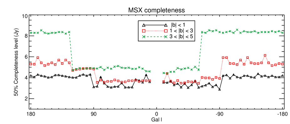
For the test points, we must use objects that span a large range of distances and extinctions, as we will need to use this function to compute the extinctions to objects at the far side of the Galaxy. For this reason, we have chosen to use young stellar clusters as the test points. They are very bright in the near-IR, and so can be observed at very large extinctions (); while spectroscopic observations of the stellar content allow the determination of both spectrophotometric and kinematic distances.
In Table 4 we list a sample of clusters with known distances and -band extinctions which we use to derive the relation between extinction and column density. For each cluster, we use the model of the Galactic electron density described in Sect. 2.1 to calculate the integrated gas column density along the line-of-sight from Earth to the cluster, . We also complement these data with that from cepheids, using the data from Berdnikov et al. (2000).
In Fig. 17 we plot against for each cluster in the sample. For the cepheids, which are all at low column densities, we take the average of the whole sample. As expected, the relation is consistent with being linear, where we find,
| (21) |
Note that if the gas distribution is altered this relation must be recalculated. To convert the -band extinction to the extinction at 21m , we must know the ratio / for interstellar extinction. Though not well studied, there seems to be some agreement in the literature that this value is 0.4-0.6 from studies of evolved stars, star-forming regions, the Galactic Centre, and the diffuse interstellar medium (Draine, 1989; Lutz, 1999; Flaherty et al., 2007; Chapman et al., 2009; Messineo et al., 2005). For the remainder of this work, we assume /.
Appendix B Completeness of the MSX survey at 21m
In order to accurately predict whether or not a source would be picked up by the MSX survey, we must first know the detection limits of the survey. The survey is not isotropic, as some regions of the sky were scanned more times than others, so we must determine the completeness as a function of viewing angle.
To measure the completeness of the MSX survey, we took representitive cutout images 1°1° in size. We then analyzed the images with the photometry package starfinder (Diolaiti et al., 2000). The input parameters were adjusted until the closest match was achieved between the starfinder and MSX source lists. The typical overlap between the sources was 80%.
Using a point-spread-function (PSF) measured from the test image, we then inserted fake stars into the image of a set brightness. No more than 40 stars were added at one time so as not to affect the crowding. We then ran the starfinder algorithm on the image and measured the recovery rate. The process was repeated five times per fake-star brightness interval, and six different brightness levels were tested between 12Jy and 2Jy. This process was repeated on a large number of fields, spaced at intervals of 5° in and 2° in , a total of 345 images in all.