The WiggleZ Dark Energy Survey: testing the cosmological model with baryon acoustic oscillations at
Abstract
We measure the imprint of baryon acoustic oscillations (BAOs) in the galaxy clustering pattern at the highest redshift achieved to date, , using the distribution of emission-line galaxies in the WiggleZ Dark Energy Survey. We quantify BAOs using three statistics: the galaxy correlation function, power spectrum and the band-filtered estimator introduced by Xu et al. (2010). The results are mutually consistent, corresponding to a measurement of the cosmic distance-redshift relation at (in terms of the acoustic parameter “” introduced by Eisenstein et al. (2005) we find ). Both BAOs and power spectrum shape information contribute toward these constraints. The statistical significance of the detection of the acoustic peak in the correlation function, relative to a wiggle-free model, is -. The ratios of our distance measurements to those obtained using BAOs in the distribution of Luminous Red Galaxies at redshifts and are consistent with a flat Cold Dark Matter model that also provides a good fit to the pattern of observed fluctuations in the Cosmic Microwave Background (CMB) radiation. The addition of the current WiggleZ data results in a improvement in the measurement accuracy of a constant equation-of-state, , using BAO data alone. Based solely on geometric BAO distance ratios, accelerating expansion () is required with a probability of , providing a consistency check of conclusions based on supernovae observations. Further improvements in cosmological constraints will result when the WiggleZ Survey dataset is complete.
keywords:
surveys, large-scale structure of Universe, cosmological parameters1 Introduction
**footnotetext: E-mail: cblake@astro.swin.edu.auThe measurement of baryon acoustic oscillations (BAOs) in the large-scale clustering pattern of galaxies has rapidly become one of the most important observational pillars of the cosmological model. BAOs correspond to a preferred length scale imprinted in the distribution of photons and baryons by the propagation of sound waves in the relativistic plasma of the early Universe (Peebles & Yu 1970, Sunyaev & Zeldovitch 1970, Bond & Efstathiou 1984, Holtzman 1989, Hu & Sugiyama 1996, Eisenstein & Hu 1998). A full account of the early-universe physics is provided by Bashinsky & Bertschinger (2001, 2002). In a simple intuitive description of the effect we can imagine an overdensity in the primordial dark matter distribution creating an overpressure in the tightly-coupled photon-baryon fluid and launching a spherical compression wave. At redshift there is a precipitous decrease in sound speed due to recombination to a neutral gas and de-coupling of the photon-baryon fluid. The photons stream away and can be mapped as the Cosmic Microwave Background (CMB) radiation; the spherical shell of compressed baryonic matter is frozen in place. The overdense shell, together with the initial central perturbation, seeds the later formation of galaxies and imprints a preferred scale into the galaxy distribution equal to the sound horizon at the baryon drag epoch. Given that baryonic matter is secondary to cold dark matter in the clustering pattern, the amplitude of the effect is much smaller than the acoustic peak structure in the CMB.
The measurement of BAOs in the pattern of late-time galaxy clustering provides a compelling validation of the standard picture that large-scale structure in today’s Universe arises through the gravitational amplification of perturbations seeded at early times. The small amplitude of the imprint of BAOs in the galaxy distribution is a demonstration that the bulk of matter consists of non-baryonic dark matter that does not couple to the relativistic plasma before recombination. Furthermore, the preferred length scale – the sound horizon at the baryon drag epoch – may be predicted very accurately by measurements of the CMB which yield the physical matter and baryon densities that control the sound speed, expansion rate and recombination time: the latest determination is Mpc (Komatsu et al. 2009). Therefore the imprint of BAOs provide a standard cosmological ruler that can map out the cosmic expansion history and provide precise and robust constraints on the nature of the “dark energy” that is apparently dominating the current cosmic dynamics (Blake & Glazebrook 2003; Hu & Haiman 2003; Seo & Eisenstein 2003). In principle the standard ruler may be applied in both the tangential and radial directions of a galaxy survey, yielding measures of the angular diameter distance and Hubble parameter as a function of redshift.
The large scale and small amplitude of the BAOs imprinted in the galaxy distribution implies that galaxy redshift surveys mapping cosmic volumes of order 1 Gpc3 with of order galaxies are required to ensure a robust detection (Tegmark 1997, Blake & Glazebrook 2003, Blake et al. 2006). Gathering such a sample represents a formidable observational challenge typically necessitating hundreds of nights of telescope time over several years. The leading such spectroscopic dataset in existence is the Sloan Digital Sky Survey (SDSS), which covers deg2 of sky containing a “main” -band selected sample of galaxies with median redshift , and a Luminous Red Galaxy (LRG) extension consisting of galaxies but covering a significantly-greater cosmic volume with median redshift . Eisenstein et al. (2005) reported a convincing BAO detection in the 2-point correlation function of the SDSS Third Data Release (DR3) LRG sample at , demonstrating that this standard-ruler measurement was self-consistent with the cosmological model established from CMB observations and yielding new, tighter constraints on cosmological parameters such as the spatial curvature. Percival et al. (2010) undertook a power-spectrum analysis of the SDSS DR7 dataset, considering both the main and LRG samples, and constrained the distance-redshift relation at both and with accuracy in units of the standard ruler scale. Other studies of the SDSS LRG sample, producing broadly similar conclusions, have been performed by Huetsi (2006), Percival et al. (2007), Sanchez et al. (2009) and Kazin et al. (2010a). Some analyses have attempted to separate the tangential and radial BAO signatures in the LRG dataset, albeit with lower statistical significance (Gaztanaga et al. 2009, Kazin et al. 2010b). These studies built on earlier hints of BAOs reported by the 2-degree Field Galaxy Redshift Survey (Cole et al. 2005) and combinations of smaller datasets (Miller et al. 2001).
This ambitious observational program to map out the cosmic expansion history with BAOs has prompted serious theoretical scrutiny of the accuracy with which we can model the BAO signature and the likely amplitude of systematic errors in the measurement. The pattern of clustering laid down in the high-redshift Universe is potentially subject to modulation by the non-linear scale-dependent growth of structure, by the distortions apparent when the signal is observed in redshift-space, and by the bias with which galaxies trace the underlying network of matter fluctuations. In this context the fact that the BAOs are imprinted on large, linear and quasi-linear scales of the clustering pattern implies that non-linear BAO distortions are relatively accessible to modelling via perturbation theory or numerical N-body simulations (Eisenstein, Seo & White 2007, Crocce & Scoccimarro 2008, Matsubara 2008). The leading-order effect is a “damping” of the sharpness of the acoustic feature due to the differential motion of pairs of tracers separated by 150 Mpc driven by bulk flows of matter. Effects due to galaxy formation and bias are confined to significantly smaller scales and are not expected to cause significant acoustic peak shifts. Although the non-linear damping of BAOs reduces to some extent the accuracy with which the standard ruler can be applied, the overall picture remains that BAOs provide a robust probe of the cosmological model free of serious systematic error. The principle challenge lies in executing the formidable galaxy redshift surveys needed to exploit the technique.
In particular, the present ambition is to extend the relatively low-redshift BAO measurements provided by the SDSS dataset to the intermediate- and high-redshift Universe. Higher-redshift observations serve to further test the cosmological model over the full range of epochs for which dark energy apparently dominates the cosmic dynamics, can probe greater cosmic volumes and therefore yield more accurate BAO measurements, and are less susceptible to the non-linear effects which damp the sharpness of the acoustic signature at low redshift and may induce low-amplitude systematic errors. Currently, intermediate redshifts have only been probed by photometric-redshift surveys which have limited statistical precision (Blake et al. 2007, Padmanabhan et al. 2007).
The WiggleZ Dark Energy Survey at the Australian Astronomical Observatory (Drinkwater et al. 2010) was designed to provide the next-generation spectroscopic BAO dataset following the SDSS, extending the distance-scale measurements across the intermediate-redshift range up to with a precision of mapping the acoustic scale comparable to the SDSS LRG sample. The survey, which began in August 2006, completed observations in January 2011 and has obtained of order redshifts for UV-bright emission-line galaxies covering of order 1000 deg2 of equatorial sky. Analysis of the full dataset is ongoing. In this paper we report intermediate results for a subset of the WiggleZ sample with effective redshift .
BAOs are a signature present in the 2-point clustering of galaxies. In this paper we analyze this signature using a variety of techniques: the 2-point correlation function, the power spectrum, and the band-filtered estimator recently proposed by Xu et al. (2010) which amounts to a band-filtered correlation function. Quantifying the BAO measurement using this range of techniques increases the robustness of our results and gives us a sense of the amplitude of systematic errors induced by our current methodologies. Using each of these techniques we measure the angle-averaged clustering statistic, making no attempt to separate the tangential and radial components of the signal. Therefore we measure the “dilation scale” distance introduced by Eisenstein et al. (2005) which consists of two parts physical angular-diameter distance, , and one part radial proper-distance, :
| (1) |
This distance measure reflects the relative importance of the tangential and radial modes in the angle-averaged BAO measurement (Padmanabhan & White 2008), and reduces to proper distance in the low-redshift limit. Given that a measurement of is correlated with the physical matter density which controls the standard ruler scale, we extract other distilled parameters which are far less significantly correlated with , namely: the acoustic parameter as introduced by Eisenstein et al. (2005); the ratio , which quantifies the distance scale in units of the sound horizon at the baryon drag epoch, ; and which is the ratio between and the distance to the CMB last-scattering surface.
The structure of this paper is as follows. The WiggleZ data sample is introduced in Section 2, and we then present our measurements of the galaxy correlation function, power spectrum and band-filtered correlation function in Sections 3, 4 and 5, respectively. The results of these different methodologies are compared in Section 6. In Section 7 we state our measurements of the BAO distance scale at using various distilled parameters, and combine our result with other cosmological datasets in Section 8. Throughout this paper we assume a fiducial cosmological model which is a flat CDM Universe with matter density parameter , baryon fraction , Hubble parameter , primordial index of scalar perturbations and redshift-zero normalization . This fiducial model is used for some of the intermediate steps in our analysis but our final cosmological constraints are, to first-order at least, independent of the choice of fiducial model.
2 Data
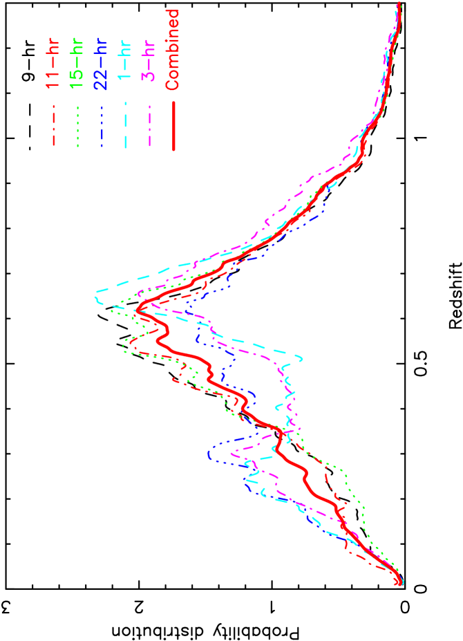
The WiggleZ Dark Energy Survey at the Anglo Australian Telescope (Drinkwater et al. 2010) is a large-scale galaxy redshift survey of bright emission-line galaxies mapping a cosmic volume of order 1 Gpc3 over the redshift interval . The survey has obtained of order redshifts for UV-selected galaxies covering of order 1000 deg2 of equatorial sky. In this paper we analyze the subset of the WiggleZ sample assembled up to the end of the 10A semester (May 2010). We include data from six survey regions in the redshift range – the 9-hr, 11-hr, 15-hr, 22-hr, 1-hr and 3-hr regions – which together constitute a total sample of galaxies. The redshift probability distributions of the galaxies in each region are shown in Figure 1.
The selection function for each survey region was determined using the methods described by Blake et al. (2010) which model effects due to the survey boundaries, incompleteness in the parent UV and optical catalogues, incompleteness in the spectroscopic follow-up, systematic variations in the spectroscopic redshift completeness across the AAOmega spectrograph, and variations of the galaxy redshift distribution with angular position. The modelling process produces a series of Monte Carlo random realizations of the angle/redshift catalogue in each region, which are used in the correlation function estimation. By stacking together a very large number of these random realizations we deduced the 3D window function grid used for power spectrum estimation.
3 Correlation function
3.1 Measurements
The 2-point correlation function is a common method for quantifying the clustering of a population of galaxies, in which the distribution of pair separations in the dataset is compared to that within random, unclustered catalogues possessing the same selection function (Peebles 1980). In the context of measuring baryon acoustic oscillations, the correlation function has the advantage that the expected signal of a preferred clustering scale is confined to a single, narrow range of separations around Mpc. Furthermore, small-scale non-linear effects, such as the distribution of galaxies within dark matter haloes, do not influence the correlation function on these large scales. One disadvantage of this statistic is that measurements of the large-scale correlation function are prone to systematic error because they are very sensitive to the unknown mean density of the galaxy population. However, such “integral constraint” effects result in a roughly constant offset in the large-scale correlation function, which does not introduce a preferred scale that could mimic the BAO signature.
In order to estimate the correlation function of each WiggleZ survey region we first placed the angle/redshift catalogues for the data and random sets on a grid of co-moving co-ordinates, assuming a flat CDM model with matter density . We then measured the redshift-space 2-point correlation function for each region using the Landy-Szalay (1993) estimator:
| (2) |
where , and are the data-data, data-random and random-random weighted pair counts in separation bin , each random catalogue containing the same number of galaxies as the real dataset. In the construction of the pair counts each data or random galaxy is assigned a weight , where is the survey number density [in Mpc-3] at the location of the th galaxy, and Mpc3 is a characteristic power spectrum amplitude at the scales of interest. The survey number density distribution is established by averaging over a large ensemble of random catalogues. The and pair counts are determined by averaging over 10 random catalogues. We measured the correlation function in 20 separation bins of width Mpc between and Mpc, and determined the covariance matrix of this measurement using lognormal survey realizations as described below. We combined the correlation function measurements in each bin for the different survey regions using inverse-variance weighting of each measurement (we note that this procedure produces an almost identical result to combining the individual pair counts).
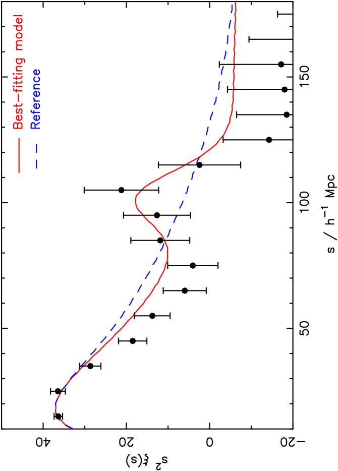
The combined correlation function is plotted in Figure 2 and shows clear evidence for the baryon acoustic peak at separation Mpc. The effective redshift of the correlation function measurement is the weighted mean redshift of the galaxy pairs entering the calculation, where the redshift of a pair is simply the average , and the weighting is where is defined above. We determined for the bin Mpc, although it does not vary significantly with separation. For the combined WiggleZ survey measurement, we found .
We note that the correlation function measurements are corrected for the effect of redshift blunders in the WiggleZ data catalogue. These are fully quantified in Section 3.2 of Blake et al. (2010), and can be well-approximated by a scale-independent boost to the correlation function amplitude of , where is the redshift blunder fraction (which is separately measured for each WiggleZ region).
3.2 Uncertainties : lognormal realizations and covariance matrix
We determined the covariance matrix of the correlation function measurement in each survey region using a large set of lognormal realizations. Jack-knife errors, implemented by dividing the survey volume into many sub-regions, are a poor approximation for the error in the large-scale correlation function because the pair separations of interest are usually comparable to the size of the sub-regions, which are then not strictly independent. Furthermore, because the WiggleZ dataset is not volume-limited and the galaxy number density varies with position, it is impossible to define a set of sub-regions which are strictly equivalent.
Lognormal realizations are relatively cheap to generate and provide a reasonably accurate galaxy clustering model for the linear and quasi-linear scales which are important for the modelling of baryon oscillations (Coles & Jones 1991). We generated a set of realizations for each survey region using the method described in Blake & Glazebrook (2003) and Glazebrook & Blake (2005). In brief, we started with a model galaxy power spectrum consistent with the survey measurement. We then constructed Gaussian realizations of overdensity fields sampled from a second power spectrum (defined below), in which real and imaginary Fourier amplitudes are drawn from a Gaussian distribution with zero mean and standard deviation . A lognormal overdensity field is then created, and is used to produce a galaxy density field consistent with the survey window function :
| (3) |
where the constant of proportionality is fixed by the size of the final dataset. The galaxy catalogue is then Poisson-sampled in cells from the density field . We note that the input power spectrum for the Gaussian overdensity field, , is constructed to ensure that the final power spectrum of the lognormal overdensity field is consistent with . This is achieved using the relation between the correlation functions of Gaussian and lognormal fields, .
We determined the covariance matrix between bins and using the correlation function measurements from a large ensemble of lognormal realizations:
| (4) |
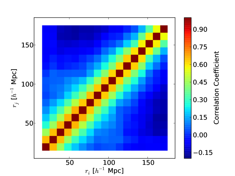
where the angled brackets indicate an average over the realizations. Figure 3 displays the final covariance matrix resulting from combining the different WiggleZ survey regions in the form of a correlation matrix . The magnitude of the first and second off-diagonal elements of the correlation matrix is typically and , respectively. We find that the jack-knife errors on scales of Mpc typically exceed the lognormal errors by a factor of , which we can attribute to an over-estimation of the number of independent jack-knife regions.
3.3 Fitting the correlation function : template model and simulations
In this Section we discuss the construction of the template fiducial correlation function model which we fitted to the WiggleZ measurement. When fitting the model we vary a scale distortion parameter , a linear normalization factor and the matter density which controls both the overall shape of the correlation function and the standard ruler sound horizon scale. Hence we fitted the model
| (5) |
The probability distribution of the scale distortion parameter , after marginalizing over and , gives the probability distribution of the distance variable where for our sample (Eisenstein et al. 2005, Padmanabhan & White 2008). , defined by Equation 1, is a composite of the physical angular-diameter distance and Hubble parameter which govern tangential and radial galaxy separations, respectively, where Mpc.
We note that the measured value of resulting from this fitting process will be independent (to first order) of the fiducial cosmological model adopted for the conversion of galaxy redshifts and angular positions to co-moving co-ordinates. A change in would result in a shift in the measured position of the acoustic peak. This shift would be compensated for by a corresponding offset in the best-fitting value of , leaving the measurement of unchanged (to first order).
An angle-averaged power spectrum may be converted into an angle-averaged correlation function using the spherical Hankel transform
| (6) |
In order to determine the shape of the model power spectrum for a given , we first generated a linear power spectrum using the fitting formula of Eisenstein & Hu (1998). This yields a result in good agreement with a CAMB linear power spectrum (Lewis, Challinor & Lasenby 2000), and also produces a wiggle-free reference spectrum which possesses the same shape as but with the baryon oscillation component deleted. This reference spectrum is useful for assessing the statistical significance with which we have detected the acoustic peak. We fixed the values of the other cosmological parameters using our fiducial model , , and . Our choices for these parameters are consistent with the latest fits to the Cosmic Microwave Background radiation (Komatsu et al. 2009).
We then corrected the power spectrum for quasi-linear effects. There are two main aspects to the model: a damping of the acoustic peak caused by the displacement of matter due to bulk flows, and a distortion in the overall shape of the clustering pattern due to the scale-dependent growth of structure (Eisenstein, Seo & White 2007, Crocce & Scoccimarro 2008, Matsubara 2008). We constructed our model in a similar manner to Eisenstein et al. (2005). We first incorporated the acoustic peak smoothing by multiplying the power spectrum by a Gaussian damping term :
| (7) |
where the inclusion of the second term maintains the same small-scale clustering amplitude. The magnitude of the damping can be modelled using perturbation theory (Crocce & Scoccimarro 2008) as
| (8) |
where is the growth rate of structure. In our fiducial cosmological model, , we find Mpc. We checked that this value was consistent with the allowed range when was varied as a free parameter and fitted to the data.
Next, we incorporated the non-linear boost to the clustering power using the fitting formula of Smith et al. (2003). However, we calculated the non-linear enhancement of power using the input no-wiggles reference spectrum rather than the full linear model including baryon oscillations:
| (9) |
Equation 9 is then transformed into a correlation function using Equation 6.
The final component of our model is a scale-dependent galaxy bias term relating the galaxy correlation function appearing in Equation 5 to the non-linear matter correlation function:
| (10) |
where we note that an overall constant normalization has already been separated in Equation 5 so that at large .
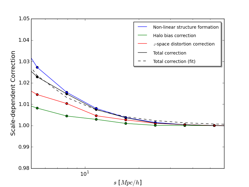
We determined the form of using halo catalogues extracted from the GiggleZ dark matter simulation. This -body simulation has been generated specifically in support of WiggleZ survey science, and consists of particles evolved in a Gpc3 box using a WMAP5 cosmology (Komatsu et al. 2009). We deduced using the non-linear redshift-space halo correlation functions and non-linear dark-matter correlation function of the simulation. We found that a satisfactory fitting formula for the scale-dependent bias over the scales of interest is
| (11) |
We performed this procedure for several contiguous subsets of halos rank-ordered by their maximum circular velocity (a robust proxy for halo mass). The best-fitting parameters of Equation 11 for the subset which best matches the large-scale WiggleZ clustering amplitude are Mpc, . We note that the magnitude of the scale-dependent correction from this term is for a scale Mpc, which is far smaller than the magnitude of such effects for more strongly-biased galaxy samples such as Luminous Red Galaxies (Eisenstein et al. 2005). This greatly reduces the potential for systematic error due to a failure to model correctly scale-dependent galaxy bias effects.
3.4 Extraction of
We fitted the galaxy correlation function template model described above to the WiggleZ survey measurement, varying the matter density , the scale distortion parameter and the galaxy bias . Our default fitting range was Mpc (following Eisenstein et al. 2005), where is an estimate of the minimum scale of validity for the quasi-linear theory described in Section 3.3. In the following, we assess the sensitivity of the parameter constraints to the fitting range.
We minimized the statistic using the full data covariance matrix, assuming that the probability of a model was proportional to . The best-fitting parameters were , and , where the errors in each parameter are produced by marginalizing over the remaining two parameters. The minimum value of is for 14 degrees of freedom (17 bins minus 3 fitted parameters), indicating an acceptable fit to the data. In Figure 2 we compare the best-fitting correlation function model to the WiggleZ data points. The results of the parameter fits are summarized for ease of reference in Table 1.
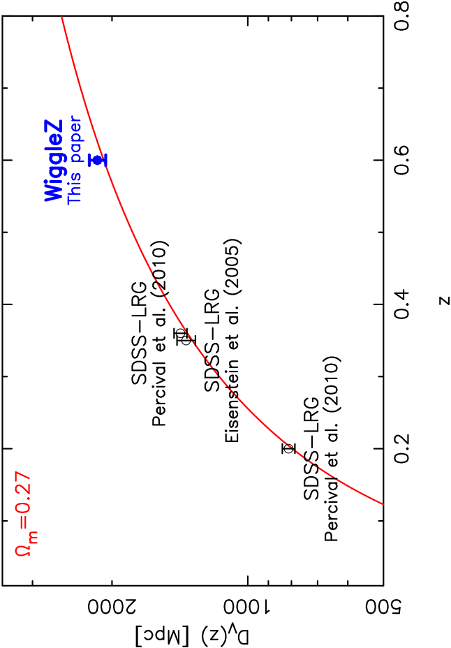
Our measurement of the scale distortion parameter may be translated into a constraint on the distance scale Mpc, corresponding to a measurement of the distance scale at . This accuracy is comparable to that reported by Eisenstein et al. (2005) for the analysis of the SDSS DR3 LRG sample at . Figure 5 compares our measurement of the distance-redshift relation with those from the LRG samples analyzed by Eisenstein et al. (2005) and Percival et al. (2010).
The 2D probability contours for the parameters and , marginalizing over , are displayed in Figure 6. Following Eisenstein et al. (2005) we indicate three degeneracy directions in this parameter space. The first direction (the dashed line in Figure 6) corresponds to a constant measured acoustic peak separation, i.e. . We used the fitting formula quoted in Percival et al. (2010) to determine as a function of (given our fiducial value of ); we find that Mpc for our fiducial cosmological model. The second degeneracy direction (the dotted line in Figure 6) corresponds to a constant measured shape of a Cold Dark Matter power spectrum, i.e. . In such models the matter transfer function at recombination can be expressed as a function of (Bardeen et al. 1986). Given that changing corresponds to a scaling of , we recover that the measured power spectrum shape depends on . The principle degeneracy axis of our measurement lies between these two curves, suggesting that both the correlation function shape and acoustic peak information are driving our measurement of . The third degeneracy direction we plot (the dash-dotted line in Figure 6), which matches our measurement, corresponds to a constant value of the acoustic parameter introduced by Eisenstein et al. (2005). We present our fits for this parameter in Section 7.
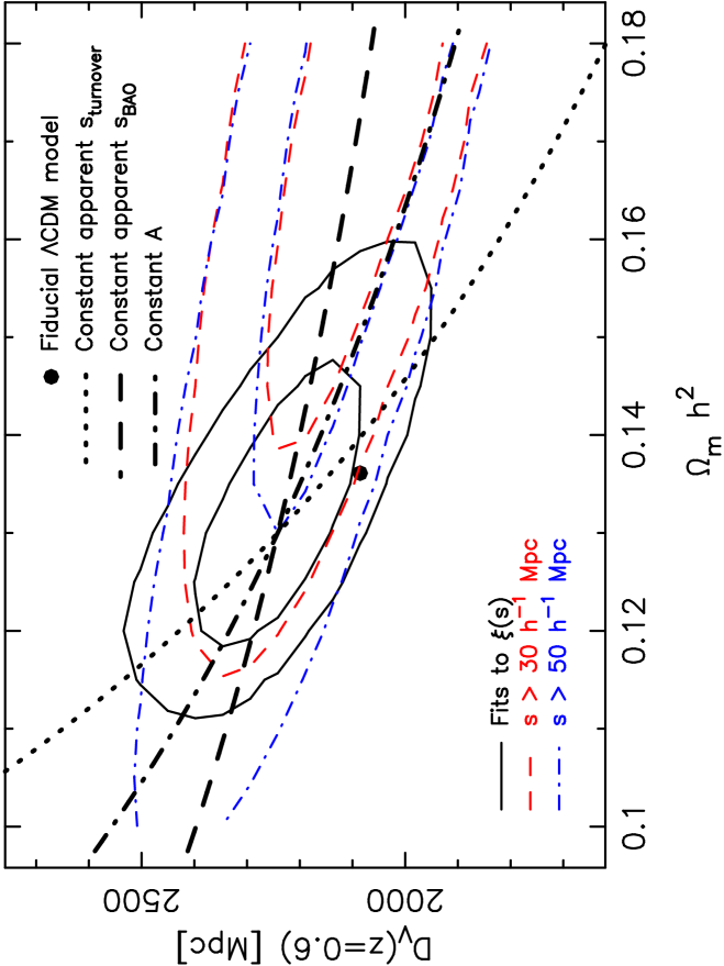
In Figure 6 we also show probability contours resulting from fits to a restricted range of separations and Mpc. In both cases the contours become significantly more extended and the long axis shifts into alignment with the case of the acoustic peak alone driving the fits. The restricted fitting range no longer enables us to perform an accurate determination of the value of from the shape of the clustering pattern alone.
3.5 Significance of the acoustic peak detection
In order to assess the importance of the baryon acoustic peak in constraining this model, we repeated the parameter fit replacing the model correlation function with one generated using a “no-wiggles” reference power spectrum , which possesses the same amplitude and overall shape as the original matter power spectrum but lacks the baryon oscillation features (i.e., we replaced with in Equation 7). The minimum value obtained for the statistic in this case was , indicating that the model containing baryon oscillations was favoured by . This corresponds to a detection of the acoustic peak with a statistical significance of -. Furthermore, the value and error obtained for the scale distortion parameter in the no-wiggles model was , representing a degradation of the error in by a factor of three. This also suggests that the acoustic peak is important for establishing the distance constraints from our measurement.
As an alternative approach for assessing the significance of the acoustic peak, we changed the fiducial baryon density to and repeated the parameter fit. The minimum value obtained for the statistic was now and the value and marginalized error determined for the scale distortion parameter was , re-affirming the significance of our detection of the baryon wiggles.
If we restrict the correlation function fits to the range Mpc, further reducing the influence of the overall shape of the clustering pattern on the goodness-of-fit, we find that our fiducial model has a minimum (for 5 degrees of freedom) and the “no-wiggles” reference spectrum produces a minimum . Even for this restricted range of scales, the model containing baryon oscillations was therefore favoured by .
3.6 Sensitivity to the clustering model
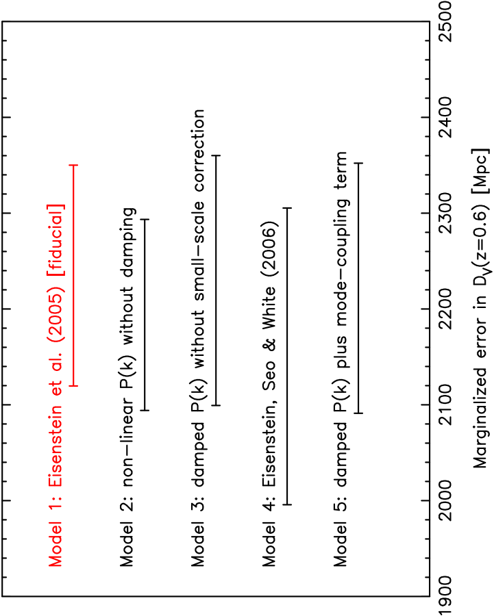
In this Section we investigate the systematic dependence of our measurement of on the model used to describe the quasi-linear correlation function. We considered five modelling approaches proposed in the literature:
-
•
Model 1: Our fiducial model described in Section 3.3 following Eisenstein et al. (2005), in which the quasi-linear damping of the acoustic peak was modelled by an exponential factor , is determined from linear theory via Equation 8, and the small-scale power was restored by adding a term multiplied by the wiggle-free reference spectrum (Equation 7).
-
•
Model 2: No quasi-linear damping of the acoustic peak was applied, i.e. .
-
•
Model 3: The term restoring the small-scale power, in Equation 7, was omitted.
-
•
Model 4: in Equation 7 was generated using Equation 14 of Eisenstein, Seo & White (2006), which implements different damping coefficients in the tangential and radial directions.
-
•
Model 5: The quasi-linear matter correlation function was generated using Equation 10 of Sanchez et al. (2009), following Crocce & Scoccimarro (2008), which includes the additional contribution of a “mode-coupling” term. We set the coefficient in this equation (rather than introduce an additional free parameter).
Figure 7 compares the measurements of from the correlation function data, marginalized over and , assuming each of these models. The agreement amongst the best-fitting measurements is excellent, and the minimum statistics imply a good fit to the data in each case. We conclude that systematic errors associated with modelling the correlation function are not significantly affecting our results. The error in the distance measurement is determined by the amount of damping of the acoustic peak, which controls the precision with which the standard ruler may be applied. The lowest distance error is produced by Model 2 which neglects damping; the greatest distance error is associated with Model 4, in which the damping is enhanced along the line-of-sight (see Equation 13 in Eisenstein, Seo & White 2006).
| Statistic | Scale range | |||||
|---|---|---|---|---|---|---|
| [Mpc] | fixing | |||||
| Mpc | ||||||
| [full] | Mpc-1 | |||||
| [wiggles] | Mpc-1 | |||||
| Mpc | ||||||
| Mpc | ||||||
| Mpc | ||||||
| [full] | Mpc-1 | |||||
| [full] | Mpc-1 | |||||
| [wiggles] | Mpc-1 | |||||
| [wiggles] | Mpc-1 | |||||
| Mpc | ||||||
| Mpc |
4 Power spectrum
4.1 Measurements and covariance matrix
The power spectrum is a second commonly-used method for quantifying the galaxy clustering pattern, which is complementary to the correlation function. It is calculated using a Fourier decomposition of the density field in which (contrary to the correlation function) the maximal signal-to-noise is achieved on large, linear or quasi-linear scales (at low wavenumbers) and the measurement of small-scale power (at high wavenumbers) is limited by shot noise. However, also in contrast to the correlation function, small-scale effects such as shot noise influence the measured power at all wavenumbers, and the baryon oscillation signature appears as a series of decaying harmonic peaks and troughs at different wavenumbers. In aesthetic terms this diffusion of the baryon oscillation signal is disadvantageous.
We estimated the galaxy power spectrum for each separate WiggleZ survey region using the direct Fourier methods introduced by Feldman, Kaiser & Peacock (1994; FKP). Our methodology is fully described in Section 3.1 of Blake et al. (2010); we give a brief summary here. Firstly we map the angle-redshift survey cone into a cuboid of co-moving co-ordinates using a fiducial flat CDM cosmological model with matter density . We gridded the catalogue in cells using nearest grid point assignment ensuring that the Nyquist frequencies in each direction were much higher than the Fourier wavenumbers of interest (we corrected the power spectrum measurement for the small bias introduced by this gridding). We then applied a Fast Fourier transform to the grid, optimally weighting each pixel by , where is the galaxy number density in the pixel (determined using the selection function) and Mpc3 is a characteristic power spectrum amplitude. The Fast Fourier transform of the selection function is then used to construct the final power spectrum estimator using Equation 13 in Blake et al. (2010). The measurement is corrected for the effect of redshift blunders using Monte Carlo survey simulations as described in Section 3.2 of Blake et al. (2010). We measured each power spectrum in wavenumber bins of width Mpc-1 between and Mpc-1, and determined the covariance matrix of the measurement in these bins by implementing the sums in Fourier space described by FKP (see Blake et al. 2010 equations 20-22). The FKP errors agree with those obtained from lognormal realizations within at all scales.
In order to detect and fit for the baryon oscillation signature in the WiggleZ galaxy power spectrum, we need to stack together the measurements in the individual survey regions and redshift slices. This requires care because each sub-region possesses a different selection function, and therefore each power spectrum measurement corresponds to a different convolution of the underlying power spectrum model. Furthermore the non-linear component of the underlying model varies with redshift, due to non-linear evolution of the density and velocity power spectra. Hence the observed power spectrum in general has a systematically-different slope in each sub-region, which implies that the baryon oscillation peaks lie at slightly different wavenumbers. If we stacked together the raw measurements, there would be a significant washing-out of the acoustic peak structure.
Therefore, before combining the measurements, we made a correction to the shape of the various power spectra to bring them into alignment. We wish to avoid spuriously enhancing the oscillatory features when making this correction. Our starting point is therefore a fiducial power spectrum model generated from the Eisenstein & Hu (1998) “no-wiggles” reference linear power spectrum, which defines the fiducial slope to which we correct each measurement. Firstly, we modified this reference function into a redshift-space non-linear power spectrum, using an empirical redshift-space distortion model fitted to the two-dimensional power spectrum split into tangential and radial bins (see Blake et al. 2011a). The redshift-space distortion is modelled by a coherent-flow parameter and a pairwise velocity dispersion parameter , which were fitted independently in each of the redshift slices. We convolved this redshift-space non-linear reference power spectrum with the selection function in each sub-region, and our correction factor for the measured power spectrum is then the ratio of this convolved function to the original real-space linear reference power spectrum. After applying this correction to the data and covariance matrix we combined the resulting power spectra using inverse-variance weighting.
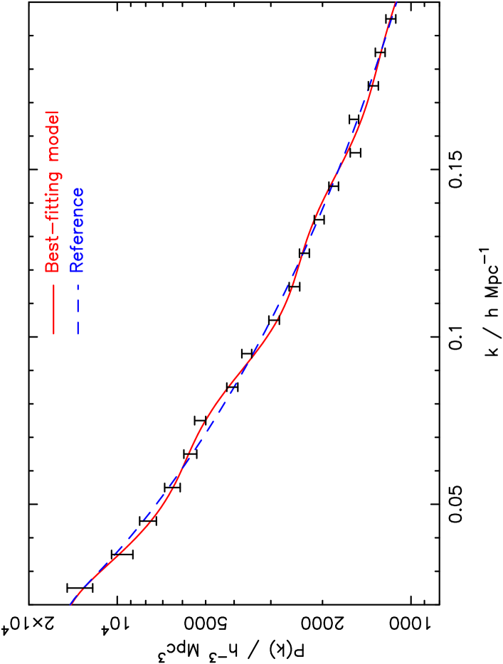
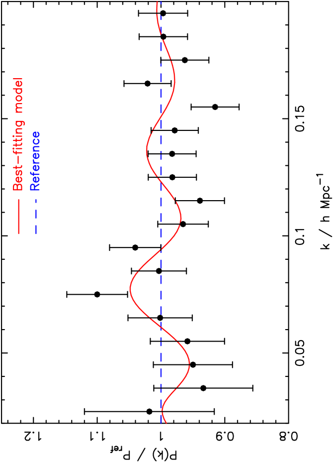
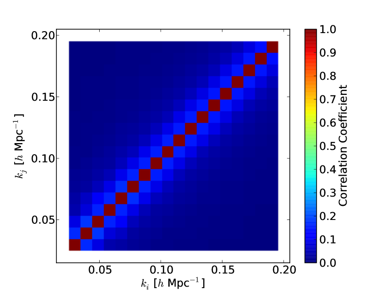
Figures 8 and 9 respectively display the combined power spectrum data, and that data divided through by the combined no-wiggles reference spectrum in order to reveal any signature of acoustic oscillations more clearly. We note that there is a significant enhancement of power at the position of the first harmonic, Mpc-1. The other harmonics are not clearly detected with the current dataset, although the model is nevertheless a good statistical fit. Figure 10 displays the final power spectrum covariance matrix, resulting from combining the different WiggleZ survey regions, in the form of a correlation matrix . We note that there is very little correlation between separate Mpc-1 power spectrum bins.
We note that our method for combining power spectrum measurements in different sub-regions only corrects for the convolution effect of the window function on the overall power spectrum shape, and does not undo the smoothing of the BAO signature in each window. We therefore expect the resulting BAO detection in the combined power spectrum may have somewhat lower significance than that in the combined correlation function.
4.2 Extraction of
We investigated two separate methods for fitting the scale distortion parameter to the power spectrum data. Our first approach used the whole shape of the power spectrum including any baryonic signature. We generated a template model non-linear power spectrum parameterized by , which we took as Equation 9 in Section 3.3, and fitted the model
| (12) |
where now appears in the denominator (as opposed to the numerator of Equation 5) due to the switch from real space to Fourier space. As in the case of the correlation function, the probability distribution of , after marginalizing over and , can be connected to the measurement of . We determined the effective redshift of the power spectrum estimate by weighting each pixel in the selection function by its contribution to the power spectrum error:
| (13) |
where is the galaxy number density in each grid cell and is the characteristic galaxy power spectrum amplitude, which we evaluated at a scale Mpc-1. We obtained an effective redshift . In order to enable comparison with the correlation function fits we applied the best-fitting value of at .
Our second approach to fitting the power spectrum measurement used only the information contained in the baryon oscillations. We divided the combined WiggleZ power spectrum data by the corresponding combined no-wiggles reference spectrum, and when fitting models we divided each trial power spectrum by its corresponding reference spectrum prior to evaluating the statistic.
We restricted our fits to Fourier wavescales Mpc-1, where the upper limit is an estimate of the range of reliability of the quasi-linear power spectrum modelling. We investigate below the sensitivity of the best-fitting parameters to the fitting range. For the first method, fitting to the full power spectrum shape, the best-fitting parameters and confidence ranges were and , where the errors in each parameter are produced by marginalizing over the remaining two parameters. The minimum value of was for 15 degrees of freedom (18 bins minus 3 fitted parameters), indicating an acceptable fit to the data. We can convert the constraint on the scale distortion parameter into a measured distance Mpc. The 2D probability distribution of and , marginalizing over , is displayed as the solid contours in Figure 11. In this Figure we reproduce the same degeneracy lines discussed in Section 3.4, which are expected to result from fits involving just the acoustic oscillations and just the shape of a pure CDM power spectrum. We note that the long axis of our probability contours is oriented close to the latter line, indicating that the acoustic peak is not exerting a strong influence on fits to the full WiggleZ power spectrum shape. Comparison of Figure 11 with Figure 6 shows that fits to the WiggleZ galaxy correlation function are currently more influenced by the BAOs than the power spectrum. This is attributable to the signal being stacked at a single scale in the correlation function, in this case of a moderate BAO detection.
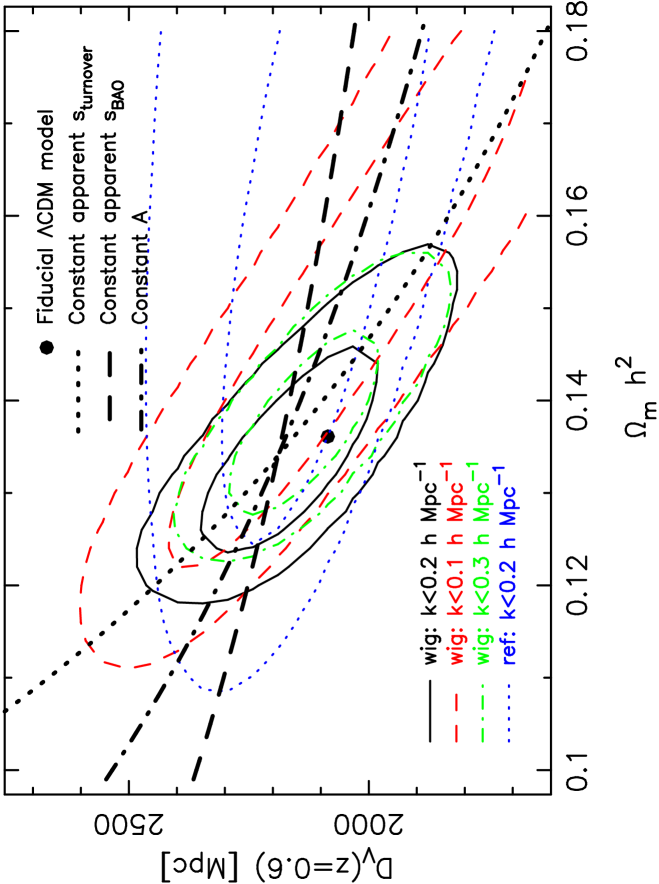
For the second method, fitting to just the baryon oscillations, the best-fitting parameters and confidence ranges were and . Inspection of the 2D probability contours of and , which are shown as the dotted contours in Figure 11, indicates that a significant degeneracy has opened up parallel to the line of constant apparent BAO scale (as expected). Increasing decreases the standard ruler scale, but the positions of the acoustic peaks may be brought back into line with the data by applying a lower scale distortion parameter . Low values of are ruled out because the resulting amplitude of baryon oscillations is too high (given that is fixed). We also plot in Figure 11 the probability contours resulting from fitting different ranges of Fourier scales Mpc-1 and Mpc-1. The confidence regions generated for these different cases overlap.
We assessed the significance with which acoustic features are detected in the power spectrum using a method similar to our treatment of the correlation function in Section 3. We repeated the parameter fit for using the “no-wiggles” reference power spectrum in place of the full model power spectrum. The minimum value obtained for the statistic in this case was , indicating that the model containing baryon oscillations was favoured by only . This is consistent with the direction of the long axis of the probability contours in Figure 11, which suggests that the baryon oscillations are not driving the fits to the full power spectrum shape.
5 Band-filtered correlation function
5.1 Measurements and covariance matrix
Xu et al. (2010) introduced a new statistic for the measurement of the acoustic peak in configuration space, which they describe as an advantageous approach for band-filtering the information. They proposed estimating the quantity
| (14) |
where is the 2-point correlation function as a function of separation and
| (15) | |||||
| (16) |
in terms of . This filter localizes the acoustic information in a single feature at the acoustic scale in a similar manner to the correlation function, which is beneficial for securing a robust, model-independent detection. However, the form of the filter function advantageously reduces the sensitivity to small-scale power (which is difficult to model due to non-linear effects) and large-scale power (which is difficult to measure because it is subject to uncertainties regarding the mean density of the sample), combining the respective advantages of the correlation function and power spectrum approaches.
Xu et al. (2010) proposed that should be estimated as a weighted sum over galaxy pairs
| (17) |
where is the separation of pair , is the cosine of the angle of the separation vector to the line-of-sight, is the number of data galaxies, and is the average galaxy density which we simply define as where is the volume of a cuboid enclosing the survey cone. The function describes the edge effects due to the survey boundaries and is normalized so that the number of random pairs in a bin is
| (18) |
where for a uniform, infinite survey. We determined the function used in Equation 17 by binning the pair counts for many random sets in fine bins of and . We then fitted a parameterized model
| (19) |
to the result in bins of , and used the coefficients to generate the value of for each galaxy pair.
We note that our Equation 17 contains an extra factor of 2 compared to Equation 12 of Xu et al. (2010) because we define the quantity as a sum over unique pairs, rather than all pairs. We also propose to modify the estimator to introduce a “DR” term by analogy with the correlation function estimator of Equation 2, in order to correct for the distribution of data galaxies with respect to the boundaries of the sample:
| (20) |
where is estimated using Equation 17, but summing over data-random pairs and excluding the initial factor of 2. We used our lognormal realizations to determine that this modified estimator of Equation 20 produces a result with lower bias and variance compared to Equation 17. We used Equation 20 to measure the band filtered correlation function of each WiggleZ region for 17 values of spaced by Mpc between and Mpc.
We determined the covariance matrix of our estimator using the ensemble of lognormal realizations for each survey region. We note that for our dataset the amplitude of the diagonal errors determined by lognormal realizations is typically times greater than jack-knife errors and times higher than obtained by evaluating Equation 13 in Xu et al. (2010) which estimates the covariance matrix in the Gaussian limit. Given the likely drawbacks of jack-knife errors (the lack of independence of the jack-knife regions on large scales) and Gaussian errors (which fail to incorporate the survey selection function), the lognormal errors should provide by far the best estimate of the covariance matrix for this measurement.
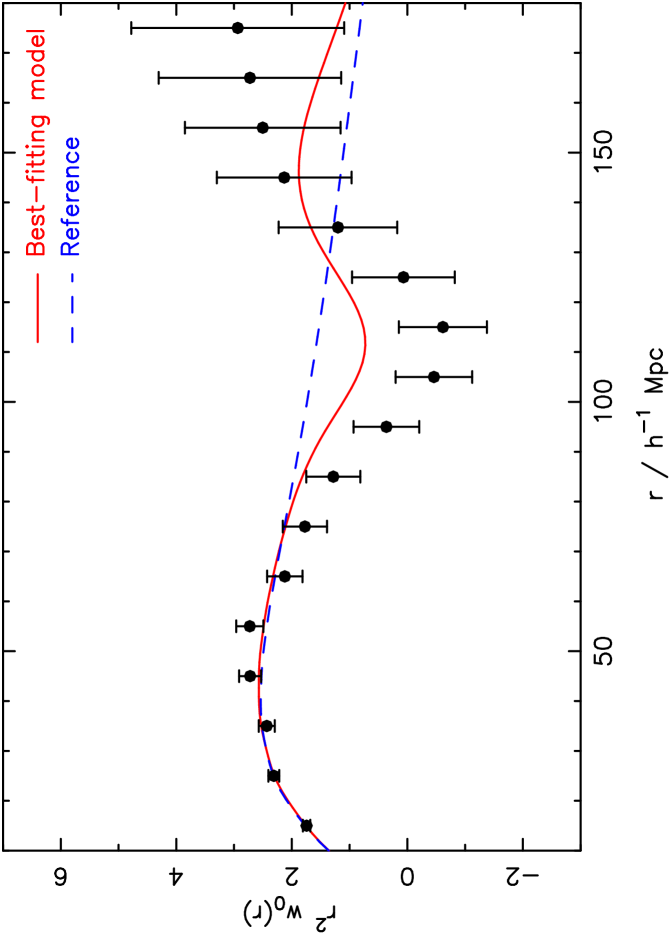
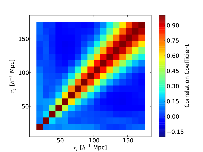
We constructed the final measurement of the band-filtered correlation function by stacking the individual measurements in different survey regions with inverse-variance weighting. Figure 12 displays our measurement. We detect clear evidence of the expected dip in at the acoustic scale. Figure 13 displays the final covariance matrix of the band-filtered correlation function resulting from combining the different WiggleZ survey regions in the form of a correlation matrix . We note that the nature of the estimator, which depends on the correlation function at all scales , implies that the data points in different bins of are highly correlated, and the correlation coefficient increases with . At the acoustic scale, neighbouring Mpc bins are correlated at the level and bins spaced by Mpc are correlated at a level of .
5.2 Extraction of
We determined the acoustic scale from the band-filtered correlation function by constructing a template function in the same style as Section 3.3 and then fitting the model
| (21) |
We determined the function by applying the transformation of Equation 14 to the template galaxy correlation function defined in Section 3.3, as a function of .
The best-fitting parameters to the band-filtered correlation function are , and , where the errors in each parameter are produced by marginalizing over the remaining two parameters. The minimum value of is for 14 degrees of freedom (17 bins minus 3 fitted parameters), indicating an acceptable fit to the data. Our measurement of the distortion parameter may be translated into a constraint on the distance scale Mpc, corresponding to a measurement of the distance scale at . Probability contours of and are overplotted in Figure 14.
In Figure 12 we compare the best fitting band-filtered correlation function model to the WiggleZ data points (noting that the strong covariance between the data gives the mis-leading impression of a poor fit). We overplot a second model which corresponds to our best-fit parameters but for which the no-wiggle reference power spectrum has been used in place of the full power spectrum. If we fit this no-wiggles model varying , and we find a minimum value of , implying that the model containing acoustic features is favoured by .
6 Comparison of clustering statistics
The distance-scale measurements of using the four different clustering statistics applied in this paper are compared in Figure 14. All four statistics give broadly consistent results for the measurement of and , with significant overlap between the respective confidence regions in this parameter space. This agreement suggests that systematic measurement errors in these statistics are not currently dominating the WiggleZ BAO fits.
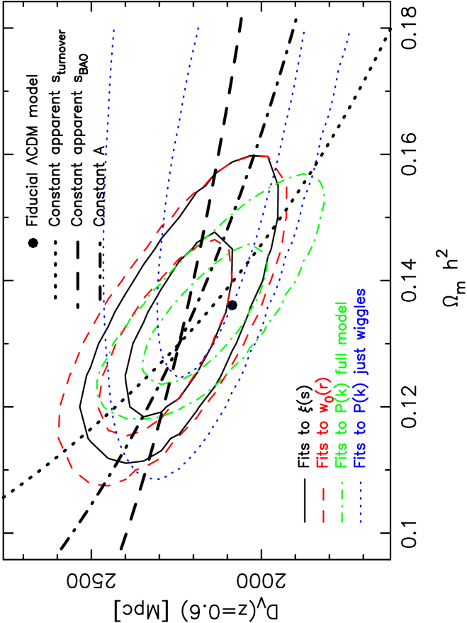
There are some differences in detail between the results derived from the four statistics. Fits to the galaxy power spectrum are currently dominated by the power spectrum shape rather than the BAOs, such that the degeneracy direction lies along the line of constant apparent turnover scale. Fitting to only the “wiggles” in Fourier space gives weaker constraints on the distance scale which (unsurprisingly) lie along the line of constant apparent BAO scale.
The correlation function and band-filtered correlation function yield very similar results (with the constraints from the standard correlation function being slightly stronger). Their degeneracy direction in the parameter space lies between the two degeneracy directions previously mentioned, implying that both the BAO scale and correlation function shape are influencing the result. The slightly weaker constraint on the distance scale provided by the band-filtered correlation function compared to the standard correlation function is likely due to the suppression of information on small and large scales by the compensated filter, which is designed to reduce potential systematic errors in modelling the shape of the clustering pattern.
For our cosmological parameter fits in the remainder of the paper we used the standard correlation function as our default choice of statistic. The correlation function provides the tightest measurement of the distance scale from our current dataset and encodes the most significant detection of the BAO signal.
7 Distilled parameters
For each of the clustering statistics determined above, the measurement of is significantly correlated with the matter density which controls both the shape of the clustering pattern and the length-scale of the standard ruler (see Figure 14). It is therefore useful to re-cast these BAO measurements in a manner less correlated with and more representative of the observable combination of parameters constrained by the BAOs. These “distilled parameters” are introduced and measured in this Section.
7.1 CMB information
The length-scale of the BAO standard ruler and shape of the linear clustering pattern is calibrated by Cosmic Microwave Background data. The cosmological information contained in the CMB may be conveniently encapsulated by the Wilkinson Microwave Anisotropy Probe (WMAP) “distance priors” (Komatsu et al. 2009). We use the 7-year WMAP results quoted in Komatsu et al. (2011).
Firstly, the CMB accurately measures the characteristic angular scale of the acoustic peaks , where is the size of the sound horizon at last scattering and is the physical angular-diameter distance to the decoupling surface. This quantity is conventionally expressed as a characteristic acoustic index:
| (22) |
The complete CMB likelihood is well-reproduced by combining this measurement of with the “shift parameter” defined by
| (23) |
and the redshift of recombination (using the fitting function given as equations 66-68 in Komatsu et al. 2009)
| (24) |
The inverse covariance matrix for is given as Table 10 in Komatsu et al. (2011) and is included in our cosmological parameter fit.
7.2 Measuring
As noted in Eisenstein et al. (2005) and discussed in Section 3.4 above, the parameter combination
| (25) |
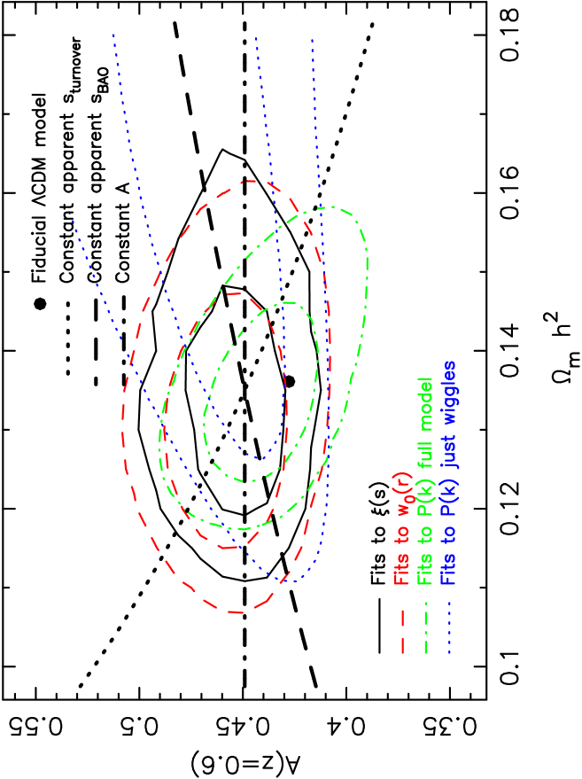
which we refer to as the “acoustic parameter”, is particularly well-constrained by distance fits which utilize a combination of acoustic oscillation and clustering shape information, since in this situation the degeneracy direction of constant lies approximately perpendicular to the minor axis of the measured probability contours. Conveniently, is also independent of (given that ). Figure 15 displays the measurements resulting from fitting the parameter set to the four WiggleZ clustering statistics and marginalizing over . The results of the parameter fits are displayed in Table 1; the correlation function yields (i.e. with a measurement precision of ). For this clustering statistic in particular, the correlation between measurements of and is very low. Given that the CMB provides a very accurate determination of (via the distance priors) we do not use the WiggleZ determination of in our cosmological parameter fits, but just use the marginalized measurement of .
The measurement of involves the assumption of a model for the shape of the power spectrum, which we parameterize by . Essentially the full power spectrum shape, rather than just the BAOs, is being used as a standard ruler, although the two features combine in such a way that and are uncorrelated. However, given that a model for the full power spectrum is being employed, we refer to these results as large-scale structure (“LSS”) rather than BAO constraints, where appropriate.
7.3 Measuring
In the case of a measurement of the BAOs in which the shape of the clustering pattern is marginalized over, the probability contours would lie along a line of constant apparent BAO scale. Hence the extracted distances are measured in units of the standard-ruler scale, which may be conveniently quoted using the distilled parameter where is the co-moving sound horizon size at the baryon drag epoch. In contrast to the acoustic parameter, provides a purely geometric distance measurement that does not depend on knowledge of the power spectrum shape. The information required to compare the observations to theoretical predictions also varies between these first two distilled parameters: the prediction of requires prior information about (or ), whereas the prediction of does not. We also fitted the parameter set to the four WiggleZ clustering statistics. The results of the parameter fits are displayed in Table 1; the correlation function yields (i.e. with a measurement precision of ). We note that, given the WiggleZ fits are in part driven by the shape of the power spectrum as well as the BAOs, there is a weak residual correlation between and .
When calculating the theoretical prediction for this parameter we obtained the value of for each cosmological model tested using Equation 6 of Eisenstein & Hu (1998), which is a fitting formula for in terms of the values of and . In our analysis we fixed which is consistent with the measured CMB value (Komatsu et al. 2009); we find that marginalizing over the uncertainty in this value does not change the results of our cosmological analysis.
We note that is determined from the matter and baryon densities in units of Mpc (not Mpc), and thus a fiducial value of must also be used when determining from data (we chose ). However, the quoted observational result is actually independent of . Adoption of a different value of would result in a shifted standard ruler scale [in units of Mpc] and hence shifted best-fitting values of and in such a way that is unchanged. However, although the observed value of is independent of the fiducial value of , the model fitted to the data still depends on as remarked above.
7.4 Measuring
The measurement of may be equivalently expressed as a ratio of the low-redshift distance to the distance to the last-scattering surface, exploiting the accurate measurement of provided by the CMB. We note that the value of depends on the behaviour of dark energy between redshift and recombination, whereas a constraint derived from only depends on the properties of dark energy at redshifts lower than . Taking the product of and approximately cancels out the dependence on the sound horizon scale:
The value is the ratio between the sound horizon at last scattering and at the baryon drag epoch. Although this is a model-dependent quantity, the change in redshift between recombination and the end of the drag epoch is driven by the relative number density of photons and baryons, which is a feature that does not change much across the range of viable cosmological models. Combining our measurement of from the WiggleZ correlation function fit with (Komatsu et al. 2011) we obtain .
7.5 Measuring distance ratios
Finally, we can avoid the need to combine the BAO fits with CMB measurements by considering distance ratios between the different redshifts at which BAO detections have been performed. Measurements of alone are dependent on the fiducial cosmological model and assumed standard-ruler scale: an efficient way to measure is by calculating , which is independent of the value of . Percival et al. (2010) reported BAO fits to the SDSS LRG sample in two correlated redshift bins and (with correlation coefficient ). Ratioing with the independent measurement of from the WiggleZ correlation function and combining the errors in quadrature we find that . Percival et al. (2010) report (where in this latter case the error is slightly tighter than obtained by adding errors in quadrature because of the correlation between and ). These two distance ratio measurements are also correlated by the common presence of in the denominators; the correlation coefficient is .
7.6 Comparison of distilled parameters
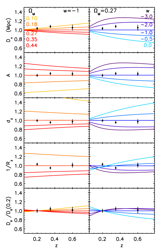
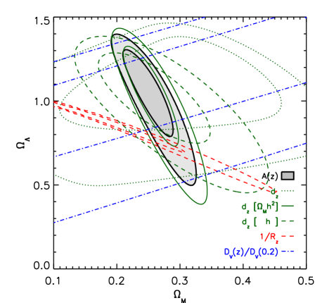
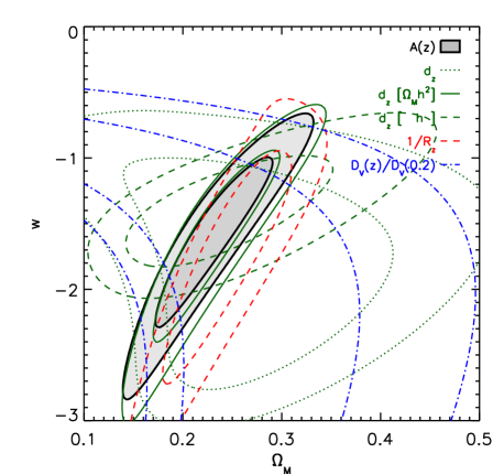
Figure 16 compares the measurements of the distilled parameters introduced in this Section, using both WiggleZ and LRG data, to a series of cosmological models varying either or the dark energy equation-of-state, , relative to a fiducial model with and . These plots have all been normalized to the fiducial model and plotted on the same scale so that the level of information contained in the different distilled parameters can be compared. For presentational purposes in Figure 16 we converted the Percival et al. (2010) measurements of into constraints on the acoustic parameter , using their fiducial values of Mpc and and employing the same fractional error in the distilled parameter.
We note that and the ratio of values are the only distilled parameters that are independent of CMB data: the measurement of uses from the CMB, and whilst the observed value of is independent of the CMB, we need to marginalize over or in order to compare it with theoretical models. Figure 17 illustrates the differing information encapsulated by each of these distilled parameters by plotting likelihood contours of for and for fitted to these data. The significant differences in the resulting likelihood contours exemplify the fact that in some cases we have not used all the information in the galaxy data (e.g. uses only the ratio of BAO scales, neglecting information from the absolute scale of the standard ruler), while in other cases we have already included significant information from the CMB (e.g. ). This illustrates that we must be careful to include additional CMB data in a self-consistent manner, not double-counting the information. This plot also serves to illustrate the mild tension between the BAO and CMB results, which can be seen from the fact that the constraints are offset from the centre of the constraints. The WiggleZ and LRG distilled BAO parameters used in these fits are summarized for convenience in Table 2.
| measured | measured | |||
|---|---|---|---|---|
| (LRG) | — | |||
| (LRG) | ||||
| (WiggleZ) |
8 Cosmological parameter measurements
In this Section we present cosmological parameter fits to the distilled BAO parameters measured above. We consider two versions of the standard cosmological model. The first version is the standard CDM model in which dark energy is a cosmological constant with equation-of-state and spatial curvature is a free parameter; we fit for and the cosmological constant density . The second version is the flat CDM model in which spatial curvature is fixed at but the equation of state of dark energy is a free parameter; we fit for and .
Unless otherwise stated, we fitted these cosmological models to the WiggleZ measurement of combined with the measurements of from LRG samples at and (Percival et al. 2010). The distilled parameter (measured from the galaxy correlation function) is the most appropriate choice for quantifying the WiggleZ BAO measurement because it is uncorrelated with , as demonstrated by Figure 15. The parameter provides the best representation of the Percival et al. (2010) BAO data, because the shape of the clustering pattern was marginalized over in that analysis.
8.1 BAO alone
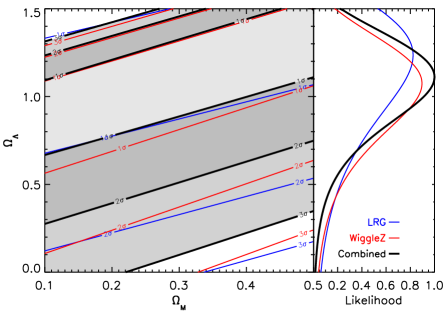
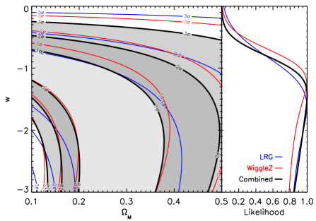
As a first step in the cosmological analysis we considered the constraints on cosmological parameters obtained using BAO data alone. Two of the distilled parameters allow the derivation of cosmological constraints based on only BAO measurements: the ratio of measurements and the acoustic parameter, .
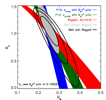
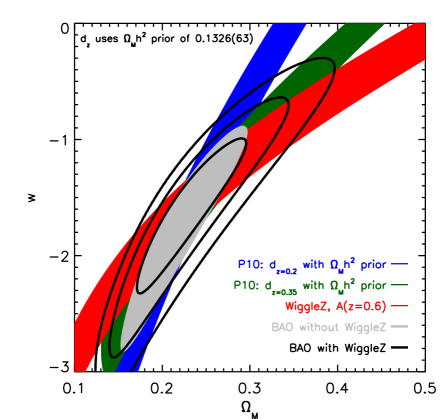
Ratios of measurements are of particularly interest because they provide constraints on the cosmic expansion history using geometric information alone, independent of the shape of the clustering pattern and the absolute scale of the standard ruler. Plots of the resulting cosmological constraints in our two test models (CDM and CDM) are shown in Figure 18. Using only LRG BAO data, the single available distance ratio provided relatively weak constraints on cosmological parameters and, in particular, could not confirm the acceleration of the expansion of the universe. The addition of the second distance ratio based on WiggleZ data, , significantly improves these constraints. For the first time, purely geometric distance ratios from BAO measurements demonstrate that the cosmic expansion is accelerating: assuming the flat CDM model, a dark energy fluid with is required with a likelihood of (assuming the flat prior ).
The improvement in the statistic comparing the best-fitting CDM model to the Einstein de-Sitter model is , whilst comparing the best-fitting CDM model to the open CDM model we obtain . Even given the extra parameter in the CDM model, information criteria tests consider this level of improvement in to be significant evidence in favour of the CDM model compared to a model with no dark energy.
Following the addition of the WiggleZ measurement, the BAO data alone require accelerating cosmic expansion with a higher level of statistical confidence than the initial luminosity distance measurements from supernovae that are considered to be the first direct evidence of accelerating expansion (compare the left-hand panel of Figure 18 with Figure 6 of Riess et al. 1998). Although these BAO measurements are not yet competitive with the latest supernova constraints, it is nevertheless reassuring that a standard-ruler measurement of the expansion of the universe, subject to an entirely different set of potential systematic uncertainties, produces a result in agreement with the standard-candle measurement.
The cosmological constraints from the acoustic parameter are much more constraining than the ratios because they implicitly incorporate a model for the clustering pattern and standard ruler scale as a function of . Figure 19 displays the resulting cosmological parameter fits to the WiggleZ measurement of combined with the LRG measurements of . For the purposes of this Figure we combine the measurements with a prior (following Percival et al. 2010); in the next sub-section we use the WMAP distance priors instead. The improvement delivered by the WiggleZ data can be seen by comparing the shaded grey contour, which is the combination of the LRG results, with the solid black contours representing the total BAO constraint including the new WiggleZ data. The current WiggleZ dataset delivers an improvement of about in the measurement of and about in the measurement of , based on LSS data alone. The marginalized parameter measurements are and (for CDM) and and (for CDM).
The BAO results continue to prefer a more negative dark energy equation-of-state or a higher cosmological constant density than the CMB or supernovae data. We explore this further in the following Section.
8.2 BAO combined with CMB and SNe
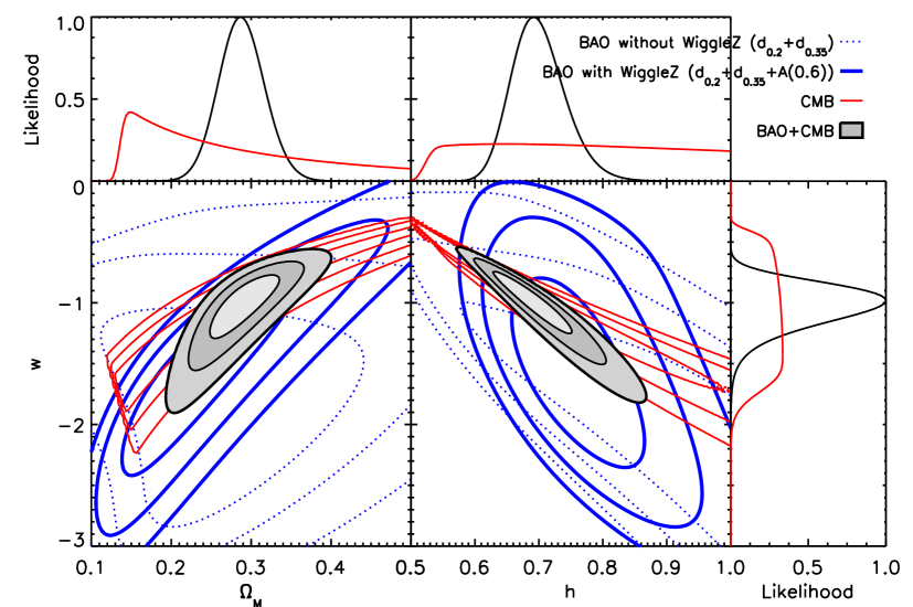
We now combine these large-scale structure (LSS) measurements with other cosmological datasets. We incorporated the CMB data using the WMAP distance priors in described in Section 7.1. We fitted a model parameterized by using flat priors , and and assuming a flat Universe (). Figure 20 compares the combined LSS cosmological parameter measurements to the CMB constraints in both the and planes, marginalizing over and respectively. The marginalized measurements of each parameter are , and .
We also combined these constraints with those arising from type Ia supernovae data from the “Union2” compilation by Amanullah et al. (2010), which includes data from Hamuy et al. (1996), Riess et al. (1999, 2007), Astier et al. (2006), Jha et al. (2006), Wood-Vasey et al. (2007), Holtzman et al. (2008), Hicken et al. (2009) and Kessler et al. (2009). Using all of these data sets (LSS+CMB+SN) the best fitting CDM model is . This model provides a a good fit to the data with a minimum per degree of freedom of 0.95.
The best-fitting parameter values based on LSS data alone are offset by slightly more than one standard deviation from the best-fitting parameter values of the combined LSS+CMB+SN fit. This mild tension between LSS and CMB+SN results was already evident in the Percival et al. (2007) measurement of BAOs in the SDSS: the LSS measurements prefer a slightly higher rate of acceleration, or a more negative equation of state of dark energy. The new WiggleZ results reported here serve to amplify that tension, although the level of discrepancy is not statistically significant.
In order to investigate whether more complex models give a better statistical fit to these datasets we performed fits of two additional cosmological models. The first is a CDM model in which we allow curvature to be a free parameter; i.e. we fit for , and . The second is a CDM model in which the equation-of-state of dark energy is allowed to vary linearly with scale factor (CPL parameterization; Chevallier & Polarski 2001, Linder 2003); i.e. we fit for , , and . If these additional parameters are justified we should find that the minimum value of the statistic decreases significantly. However, we in fact find that the addition of the extra degrees of freedom improves the value of the best-fitting model by at most compared to the CDM model, and significantly degrades the errors in our fitted parameters. In terms of information criteria this does not represent a sufficient improvement to justify the addition of the extra degree-of-freedom.
9 Conclusions
We summarize our conclusions as follows:
-
•
This intermediate sample of the WiggleZ Dark Energy Survey, containing galaxies, permits a convincing detection of baryon acoustic oscillations at the highest redshift achieved to date, . We have quantified the baryon oscillations in both the galaxy correlation function and power spectrum statistics. The statistical significance of the correlation function detection exceeds 3-.
-
•
We present the first measurement from a galaxy survey of the band-filtered BAO estimator defined by Xu et al. (2010), which also exhibits strong evidence of BAOs, and we suggest some improvements in its implementation. The distance-scale measurements resulting from are slightly less precise than those obtained by fits to the standard correlation function, likely due to the suppression by the filtering function of clustering information on small and large scales.
-
•
The clustering statistics are well-fit by a non-linear power spectrum model including a Gaussian damping factor which models coherent flows on 100 Mpc scales. We show that our results are not sensitive to the details of the quasi-linear model by comparing five different implementations suggested in the literature. We use the GiggleZ N-body simulation to demonstrate that scale-dependent bias effects in the WiggleZ galaxy distribution have an amplitude of on Mpc scales, compared to for more highly-biased LRGs.
-
•
We measured the distance-redshift relation with an accuracy of about using the scale dilation method. The self-consistency of the measurement amongst the independent clustering statistics suggests that systematic measurement errors are not dominating these results. Our data best constrain the quantity , which lies perpendicular to the principal degeneracy direction of our contours and which is measured with an accuracy of : we find .
-
•
The distance ratios between our measurements and previous analyses of the Luminous Red Galaxy distribution at redshifts and are consistent with a flat CDM cosmological model which also provides a good fit to the CMB distance priors. Addition of the WiggleZ data allows us to establish, using geometric distance ratios alone, that the equation-of-state of dark energy drives an accelerating expansion () with likelihood, assuming a flat prior . The current WiggleZ dataset delivers an improvement of about in the measurement of and in the measurement of , based on BAO data alone. The WiggleZ measurement confirms the mild tension that was previously reported between CMB and BAO measurements of the acceleration of the Universe, whereby the BAO data favour a slightly higher acceleration rate.
-
•
Cosmological parameter fits using BAO and CMB data are consistent with those based on current supernovae data; this cross-check does not yield evidence for systematic errors. Combining all current BAO, CMB and supernovae data we find that the best-fitting CDM model is . These data do not justify the addition of another degree-of-freedom such as non-zero spatial curvature or an evolving equation-of-state of dark energy.
When the complete BAO dataset from the WiggleZ survey is available, we plan to split our data into redshift bins and explore fitting for the BAOs separately in the tangential and radial directions, improving the cosmological constraints presented in this paper.
The WiggleZ dataset enables further tests of the cosmological model, complementary to those involving baryon acoustic oscillations. Two such results will be published at a similar time as the current paper. Firstly, we have used redshift-space distortions in the WiggleZ sample to measure accurately the growth rate of structure in the redshift range , finding that this is consistent with the predictions of the CDM model (Blake et al. 2011a). Secondly, we have used the Alcock-Paczynski test to perform non-parametric reconstructions of the cosmic expansion history (Blake et al. 2011b).
Acknowledgments
We acknowledge financial support from the Australian Research Council through Discovery Project grants funding the positions of SB, MP, GP and TD. SMC acknowledges the support of the Australian Research Council through a QEII Fellowship. MJD thanks the Gregg Thompson Dark Energy Travel Fund for financial support.
GALEX (the Galaxy Evolution Explorer) is a NASA Small Explorer, launched in April 2003. We gratefully acknowledge NASA’s support for construction, operation and science analysis for the GALEX mission, developed in co-operation with the Centre National d’Etudes Spatiales of France and the Korean Ministry of Science and Technology.
Finally, the WiggleZ survey would not be possible without the dedicated work of the staff of the Australian Astronomical Observatory in the development and support of the AAOmega spectrograph, and the running of the AAT.
References
- [1] Amanullah R., et al., 2010, ApJ, 716, 712
- [2] Astier P., et al., 2006, A&A, 447, 31
- [3] Bardeen J.M., Bond J.R., Kaiser N., Szalay A.S., 1986, ApJ, 304, 15
- [4] Bashinsky S., Bertschinger E., 2001, Phys. Rev. Lett., 87, 081301
- [5] Bashinsky S., Bertschinger E., 2002, Phys. Rev. D, 65, 123008
- [6] Blake C.A, Glazebrook K., 2003, ApJ, 594, 665
- [7] Blake C.A., Parkinson D., Bassett B., Glazebrook K., Kunz M., Nichol R.C., 2006, MNRAS, 365, 255
- [8] Blake C.A., Collister A., Bridle S., Lahav O., 2007, MNRAS, 374, 1527
- [9] Blake C.A., et al., 2010, MNRAS, 406, 803
- [10] Blake C.A., et al., 2011a, MNRAS accepted
- [11] Blake C.A., et al., 2011b, MNRAS submitted
- [12] Bond J.R., Efstathiou G., 1984, ApJ, 285, L45
- [13] Chevallier M., Polarski D., 2001, Int. J. Mod. Phys., D10, 213
- [14] Cole S. et al., 2005, MNRAS, 362, 505
- [15] Coles P., Jones B., 1991, MNRAS, 248, 1
- [16] Crocce M., Scoccimarro R., 2008, Phys. Rev. D, 2008, 77, 3533
- [17] Drinkwater M., et al., 2010, MNRAS, 401, 1429
- [18] Eisenstein D.J., Hu W., 1998, ApJ, 518, 2
- [19] Eisenstein D.J. et al., 2005, ApJ, 633, 560
- [20] Eisenstein D.J., Seo H.-J., White M., 2007, ApJ, 664, 660
- [21] Feldman H.A., Kaiser N., Peacock J.A., 1994, ApJ, 426, 23
- [22] Gaztanaga E., Cabre A., Hui L., 2009, MNRAS, 399, 1663
- [23] Glazebrook K., Blake C.A., 2005, ApJ, 631, 1
- [24] Hamuy M., et al., 1996, AJ, 112, 2408
- [25] Hicken M., et al., 2009, ApJ, 700, 331
- [26] Holtzman J.A., 1989, ApJS, 71, 1
- [27] Holtzman J.A., et al. 2008, AJ, 136, 2306
- [28] Hu W., Haiman Z., 2003, Phys. Rev. D, 68, 063004
- [29] Hu W., Sugiyama N., 1996, ApJ, 471, 542
- [30] Huetsi G., 2006, A&A, 449, 891
- [31] Jha S., et al., 2006, AJ, 131, 527
- [32] Kazin E., et al., 2010a, ApJ, 710, 1444
- [33] Kazin E., Blanton M.R., Scoccimarro R., McBride C.K., Berlind A.A., 2010b, ApJ, 719, 1032
- [34] Kessler R., et al., 2009, ApJS, 185, 32
- [35] Komatsu E., et al., 2009, ApJS, 180, 330
- [36] Komatsu E., et al., 2011, ApJS, 192, 18
- [37] Landy S.D., Szalay A.S., 1993, ApJ, 412, 64
- [38] Lewis A., Challinor A., Lasenby A., 2000, ApJ, 538, 473
- [39] Linder E.V., 2003, PRL, 90, 091301
- [40] Matsubara T., 2008, Phys. Rev. D, 78, 083519
- [41] Miller C.J., Nichol R.C., Batuski D.J., 2001, ApJ, 555, 68
- [42] Padmanabhan N. et al., 2007, MNRAS, 378, 852
- [43] Padmanabhan N., White M., 2008, Phys. Rev. D, 77, 3540
- [44] Peebles P.J.E., Yu J.T., 1970, ApJ, 162, 815
- [45] Peebles P.J.E., 1980, The Large-Scale Structure of the Universe, Princeton Univ. Press, Princeton, NJ
- [46] Percival W.J., et al., 2007, ApJ, 657, 51
- [47] Percival W.J., et al., 2010, MNRAS, 401, 2148
- [48] Riess A.G., et al., 1998, AJ, 116, 1009
- [49] Riess A.G., et al., 1999, AJ, 117, 707
- [50] Riess A.G., et al., 2007, ApJ, 659, 98
- [51] Sanchez A.G., Crocce M., Cabre A., Baugh C.M., Gaztanaga E., 2009, MNRAS, 400, 1643
- [52] Seo H.-J., Eisenstein D.J., 2003, ApJ, 598, 720
- [53] Smith R.E. et al., 2003, MNRAS, 341, 1311
- [54] Sunyaev R.A., Zeldovitch, Y.B., 1970, Ap&SS, 7, 3
- [55] Tegmark M., 1997, PRL, 79, 20
- [56] Wood-Vasey W.M., et al., 2007, ApJ, 666, 694
- [57] Xu X., et al., 2010, ApJ, 718, 1224