Multibody Multipole Methods

Dongryeol Lee Computational Science and Engineering
Georgia Institute of Technology
266 Ferst Drive
Atlanta, GA 30332
Arkadas Ozakin Georgia Tech Research Institute
Georgia Institute of Technology
266 Ferst Drive
Atlanta, GA 30332
Alexander G. Gray
Abstract

A three-body potential function can account for interactions among triples of particles which are uncaptured by pairwise interaction functions such as Coulombic or Lennard-Jones potentials. Likewise, a multibody potential of order n𝑛n can account for interactions among n𝑛n-tuples of particles uncaptured by interaction functions of lower orders. To date, the computation of multibody potential functions for a large number of particles has not been possible due to its O(Nn)𝑂superscript𝑁𝑛O(N^{n}) scaling cost. In this paper we describe a fast tree-code for efficiently approximating multibody potentials that can be factorized as products of functions of pairwise distances. For the first time, we show how to derive a Barnes-Hut type algorithm for handling interactions among more than two particles. Our algorithm uses two approximation schemes: 1) a deterministic series expansion-based method; 2) a Monte Carlo-based approximation based on the central limit theorem. Our approach guarantees a user-specified bound on the absolute or relative error in the computed potential with an asymptotic probability guarantee. We provide speedup results on a three-body dispersion potential, the Axilrod-Teller potential.

keywords:
Fast multipole methods; Data structures; kd-trees; Axilrod-Teller potential; Multi-tree algorithms
journal: Journal of Computational Physics

1 Introduction

In this paper, we generalize previous algorithmic frameworks for rapidly computing pair-wise summations to include higher-order summations. Suppose we are given a set of particles X={x0,,xN1}𝑋subscript𝑥0subscript𝑥𝑁1X=\{x_{0},\cdots,x_{N-1}\} in D𝐷D-dimensional space.

Refer to caption
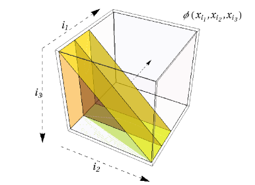
Figure 1: An example multibody computation (n=3𝑛3n=3). For each fixed argument xi1subscript𝑥subscript𝑖1x_{i_{1}}, Φ(xi1)Φsubscript𝑥subscript𝑖1\Phi(x_{i_{1}}) equals the summation of the entries ϕ(xi1,xi2,xi3)italic-ϕsubscript𝑥subscript𝑖1subscript𝑥subscript𝑖2subscript𝑥subscript𝑖3\phi(x_{i_{1}},x_{i_{2}},x_{i_{3}}) in the shaded region corresponding to xi1subscript𝑥subscript𝑖1x_{i_{1}}.

For xX𝑥𝑋x\in X and a n𝑛n-tuple function ϕ:D××Dn copies:italic-ϕsubscriptsuperscript𝐷superscript𝐷𝑛 copies\phi:\underbrace{\mathbb{R}^{D}\times\cdots\times\mathbb{R}^{D}}_{n\mbox{ copies}}\rightarrow\mathbb{R}, we are interested in computing the following form111In computing Φ(x)Φ𝑥\Phi(x), we fix one of the arguments of ϕitalic-ϕ\phi as x𝑥x and choose a (n1)𝑛1(n-1)-subset from X(n1)superscript𝑋𝑛1X^{(n-1)} which does not contain x𝑥x.:

Φ(x;X××X(n1) copies)=xi2X\{x}xi3X\{x}i2<i3xinX\{x}in1<inϕ(x,xi2,xin)Φ𝑥subscript𝑋𝑋𝑛1 copiessubscriptsubscript𝑥subscript𝑖2\𝑋𝑥subscriptsubscript𝑥subscript𝑖3\𝑋𝑥subscript𝑖2subscript𝑖3subscriptsubscript𝑥subscript𝑖𝑛\𝑋𝑥subscript𝑖subscript𝑛1subscript𝑖𝑛italic-ϕ𝑥subscript𝑥subscript𝑖2subscript𝑥subscript𝑖𝑛\Phi(x;\underbrace{X\times\cdots\times X}_{(n-1)\mbox{ copies}})=\sum\limits_{x_{i_{2}}\in X\backslash\{x\}}\ \sum\limits_{\begin{subarray}{c}x_{i_{3}}\in X\backslash\{x\}\\ i_{2}<i_{3}\end{subarray}}\cdots\sum\limits_{\begin{subarray}{c}x_{i_{n}}\in X\backslash\{x\}\\ i_{n_{1}}<i_{n}\end{subarray}}\phi(x,x_{i_{2}}\cdots,x_{i_{n}}) (1)

Sums of the form Equation (1) occur in molecular dynamics, protein structure prediction, and other similar contexts. Biomolecular simulations usually break down the interactions in complex chemical systems into balls-and-springs mechanical models augmented by torsional terms, pairwise point charge electrostatic terms, and simple pairwise dispersion (van der Waals) interactions, etc. However, such pairwise (n=2𝑛2n=2) interactions often fail to capture important, complex non-additive interactions found in real systems. Though many researchers have argued that multibody potentials enable more accurate and realistic molecular modeling, the evaluation of n𝑛n-body forces for n3𝑛3n\geq 3 in systems beyond tiny sizes (less than 10,000 particles) has not been possible due to the unavailability of an efficient way to realize the computation.

In this paper we focus on computing multibody potentials of the third order (n=3𝑛3n=3), but frame our presentation so that the methods can easily be generalized to handle higher-order potentials. For concreteness, we consider the Axilrod-Teller potential (dispersion potential):

ϕ(xi,xj,xk)=1+3cosθicosθjcosθkxixj3xixk3xjxk3italic-ϕsubscript𝑥𝑖subscript𝑥𝑗subscript𝑥𝑘13subscript𝜃𝑖subscript𝜃𝑗subscript𝜃𝑘superscriptnormsubscript𝑥𝑖subscript𝑥𝑗3superscriptnormsubscript𝑥𝑖subscript𝑥𝑘3superscriptnormsubscript𝑥𝑗subscript𝑥𝑘3\phi(x_{i},x_{j},x_{k})=\frac{1+3\cos{\theta_{i}}\cos{\theta_{j}}\cos{\theta_{k}}}{||x_{i}-x_{j}||^{3}||x_{i}-x_{k}||^{3}||x_{j}-x_{k}||^{3}} (2)

where θisubscript𝜃𝑖\theta_{i}, θjsubscript𝜃𝑗\theta_{j}, θksubscript𝜃𝑘\theta_{k} are the angles at the vertices of the triangle xixjxksubscript𝑥𝑖subscript𝑥𝑗subscript𝑥𝑘x_{i}x_{j}x_{k} and ||||||\cdot|| is the Euclidean distance metric. This potential [1] describes induced dipole interactions between triples of atoms, and is known to be important for the accurate computation of the physical properties of certain noble gases.

This Paper. For the first time, we introduce a fast algorithm for efficiently computing multibody potentials for a large number of particles. We restrict the class of multibody potentials to those that can be factorized as products of functions of pairwise Euclidean distances. That is,

ϕ(xi1,,xin)=1p<qnϕp,q(xip,xiq)=1p<qnϕp,q(xipxiq)italic-ϕsubscript𝑥subscript𝑖1subscript𝑥subscript𝑖𝑛subscriptproduct1𝑝𝑞𝑛subscriptitalic-ϕ𝑝𝑞subscript𝑥subscript𝑖𝑝subscript𝑥subscript𝑖𝑞subscriptproduct1𝑝𝑞𝑛subscriptitalic-ϕ𝑝𝑞subscript𝑥subscript𝑖𝑝subscript𝑥subscript𝑖𝑞\phi(x_{i_{1}},\cdots,x_{i_{n}})=\prod\limits_{1\leq p<q\leq n}\phi_{p,q}(x_{i_{p}},x_{i_{q}})=\prod\limits_{1\leq p<q\leq n}\phi_{p,q}(x_{i_{p}}-x_{i_{q}}) (3)

Our algorithm achieves speedup by utilizing two approximation methods: a deterministic and a probabilistic one. The deterministic approximation is based on the analytic series-expansion-based approach in [2, 3, 4] to handle potential functions that describe n𝑛n-body interactions with n>2𝑛2n>2. The probabilistic approach uses a Monte Carlo-based approximation based on the central limit theorem. Our algorithm can compute multibody potentials within user-specified bounds for relative or absolute error with an asymptotic probability guarantee.

However, we would like to point out the following limitations in our algorithm. First of all, we do not present a full-fledged derivation of all three translation operators (namely the far-to-far, the far-to-local, and the local-to-local translation operators) for the general multibody case. While we define the far-field expansion for a restricted class of multibody potentials, defining the local expansion for this same class is harder (see Section 3.4). We would also like to point out that the hybrid deterministic/probabilistic approximation heuristic works under some partial distributions but not all. Indeed, there are configurations for which the speedup factor over the naive brute-force method is minimal. The Monte-Carlo based approximation relies on two theorems: 1) the central limit theorem from which we determine the number of required samples; 2) the Berry-Esseen theorem which characterizes the the rate at which the sample average converges to the true average. Both theorems provide only asymptotic guarantees.

Our work utilizes and extends a framework for efficient algorithms for so-called generalized N𝑁N-Body Problems [5], which introduced multi-tree methods. The framework was originally developed to accelerate common bottleneck statistical computations based on distances; it utilizes multiple kd𝑘𝑑kd-trees and other spatial data structures to reduce computation times both asymptotically and practically by multiple orders of magnitude. This work extends the framework with higher-order hierarchical series approximation techniques, demonstrating a fast multipole-type method for higher-order interactions for the first time, effectively creating a Multibody Multipole Method.

Section 3 introduces the generalized N𝑁N-body framework and describes a partial extension of fast multipole-type methods to handle higher-order interactions; we will discuss the technical difficulties for deriving all of the necessary tools for the general multibody case. As a result, we utilize only a simple but effective approximation using the center-of-mass approximations. Section 4 focuses on three-body interactions and introduces methods to do potential computations under both deterministic and probabilistic error criteria; the section also provides a description of the fast algorithm for the three-body case. Section 5 proves that our proposed algorithms can approximate potentials within user-specified error bounds. Section 6 shows experimental scalability results for our proposed algorithms against the naive algorithm under different error parameter settings.

Notations. Throughout this paper, we use these common sets of notations:

  • 1.

    (Normal Distribution). This is denoted by 𝒩(μ,Σ)𝒩𝜇Σ\mathcal{N}(\mu,\Sigma) where μ𝜇\mu and ΣΣ\Sigma are the mean and the covariance respectively.

  • 2.

    (Vector Component). For a given vector vk𝑣superscript𝑘v\in\mathbb{R}^{k}, we access its d𝑑d-th component by v[d]𝑣delimited-[]𝑑{v}[d] where 1dk1𝑑𝑘1\leq d\leq k (i.e. 111-based index).

  • 3.

    (Multi-index Notation). Throughout this paper, we will be using the multi-index notation. A D𝐷D-dimensional multi-index 𝜶𝜶\bm{\alpha} is a D𝐷D-tuple of non-negative integers and will be denoted using a bold lowercase Greek alphabet. For any D𝐷D-dimensional multi-indices 𝜶𝜶\bm{\alpha}, 𝜷𝜷\bm{\beta} and any xD𝑥superscript𝐷{x}\in\mathbb{R}^{D},

    • |𝜶|=𝜶[1]+𝜶[2]++𝜶[D]𝜶𝜶delimited-[]1𝜶delimited-[]2𝜶delimited-[]𝐷|\bm{\alpha}|=\bm{\alpha}[1]+\bm{\alpha}[2]+\cdots+\bm{\alpha}[D]

    • 𝜶!=(𝜶[1])!(𝜶[2])!(𝜶[D])!𝜶𝜶delimited-[]1𝜶delimited-[]2𝜶delimited-[]𝐷\bm{\alpha}!=(\bm{\alpha}[1])!(\bm{\alpha}[2])!\cdots(\bm{\alpha}[D])!

    • x𝜶=(x[1])𝜶[1](x[2])𝜶[2](x[D])𝜶[D]superscript𝑥𝜶superscript𝑥delimited-[]1𝜶delimited-[]1superscript𝑥delimited-[]2𝜶delimited-[]2superscript𝑥delimited-[]𝐷𝜶delimited-[]𝐷{x}^{\bm{\alpha}}=({x}[1])^{\bm{\alpha}[1]}({x}[2])^{\bm{\alpha}[2]}\cdots({x}[D])^{\bm{\alpha}[D]}

    • D𝜶=1𝜶[1]2𝜶[2]D𝜶[D]superscript𝐷𝜶superscriptsubscript1𝜶delimited-[]1superscriptsubscript2𝜶delimited-[]2superscriptsubscript𝐷𝜶delimited-[]𝐷D^{\bm{\alpha}}=\partial_{1}^{\bm{\alpha}[1]}\partial_{2}^{\bm{\alpha}[2]}\cdots\partial_{D}^{\bm{\alpha}[D]}

    • 𝜶+𝜷=(𝜶[1]+𝜷[1],,𝜶[D]+𝜷[D])𝜶𝜷𝜶delimited-[]1𝜷delimited-[]1𝜶delimited-[]𝐷𝜷delimited-[]𝐷\bm{\alpha}+\bm{\beta}=(\bm{\alpha}[1]+\bm{\beta}[1],\cdots,\bm{\alpha}[D]+\bm{\beta}[D])

    • 𝜶𝜷=(𝜶[1]𝜷[1],,𝜶[D]𝜷[D])𝜶𝜷𝜶delimited-[]1𝜷delimited-[]1𝜶delimited-[]𝐷𝜷delimited-[]𝐷\bm{\alpha}-\bm{\beta}=(\bm{\alpha}[1]-\bm{\beta}[1],\cdots,\bm{\alpha}[D]-\bm{\beta}[D]) for 𝜶𝜷𝜶𝜷\bm{\alpha}\geq\bm{\beta}.

    where isubscript𝑖\partial_{i} is a i𝑖i-th directional partial derivative. Define 𝜶>𝜷𝜶𝜷\bm{\alpha}>\bm{\beta} if 𝜶[d]>𝜷[d]𝜶delimited-[]𝑑𝜷delimited-[]𝑑\bm{\alpha}[d]>\bm{\beta}[d], and 𝜶p𝜶𝑝\bm{\alpha}\geq p for p+{0}𝑝superscript0p\in\mathbb{Z^{+}}\cup\{0\} if 𝜶[d]p𝜶delimited-[]𝑑𝑝\bm{\alpha}[d]\geq p for 1dD1𝑑𝐷1\leq d\leq D (and similarly for 𝜶p𝜶𝑝\bm{\alpha}\leq p).

  • 4.

    (Size of a Point Set). Given a set S𝑆S, it size is denoted by |S|𝑆|S|.

  • 5.

    (Probability Guarantee). We use the unbold Greek alphabet α𝛼\alpha.

  • 6.

    (A Tree Node). A tree node represents a subset of a point set represented by the root node. Hence, we use the same notation as the previous.

  • 7.

    (Representative Point of a Tree Node). Usually a geometric center is used but any point inside the bounding primitive of a tree node is chosen as well. For the tree node P𝑃{P}, this is denoted as cPsubscript𝑐𝑃{c_{P}}.

  • 8.

    (Child Nodes of an Internal Tree Node). Given a node N𝑁{N}, denote its left and right child nodes by NLsuperscript𝑁𝐿{N}^{L} and NRsuperscript𝑁𝑅{N}^{R} respectively.

2 Related Work

2.1 Error Bounds

Due to its expensive computational cost, many algorithms approximate sums at the expense of reduced precision. The following error bounding criteria are used in the literature:

Definition 2.1.

τ𝜏\tau absolute error bound: For each Φ(x)Φ𝑥\Phi(x) for xX𝑥𝑋x\in X, it computes Φ~(x)~Φ𝑥\widetilde{\Phi}(x) such that |Φ~(x)Φ(x)|τ~Φ𝑥Φ𝑥𝜏\left|\widetilde{\Phi}(x)-\Phi(x)\right|\leq\tau.

Definition 2.2.

ϵitalic-ϵ\epsilon relative error bound: For each Φ(x)Φ𝑥\Phi(x) for xX𝑥𝑋x\in X, compute Φ~(x)~Φ𝑥\widetilde{\Phi}(x) such that |Φ~(x)Φ(x)|ϵ|Φ(x)|~Φ𝑥Φ𝑥italic-ϵΦ𝑥\left|\widetilde{\Phi}(x)-\Phi(x)\right|\leq\epsilon\left|\Phi(x)\right|.

Bounding the relative error is much harder because the error bound criterion is in terms of the initially unknown exact quantity. As a result, many previous methods [4, 6] have focused on bounding the absolute error. The relative error bound criterion is preferred to the absolute error bound criterion in statistical applications in which high accuracy is desired. Our framework can enforce the following error form:

Definition 2.3.

(1α)1𝛼(1-\alpha) probabilistic ϵitalic-ϵ\epsilon relative/τ𝜏\tau absolute error: For each Φ(x)Φ𝑥\Phi(x) for xX𝑥𝑋x\in X, compute Φ~(x)~Φ𝑥\widetilde{\Phi}(x), such that with at least probability 0<1α101𝛼10<1-\alpha\leq 1, |Φ~(x)Φ(x)|ϵ|Φ(x)|+τ~Φ𝑥Φ𝑥italic-ϵΦ𝑥𝜏\left|\widetilde{\Phi}(x)-\Phi(x)\right|\leq\epsilon\left|\Phi(x)\right|+\tau.

2.2 Series Expansion

A series of papers first laid the foundations for efficiently computing sums of pairwise potentials such as Coulombic and Yukawa potentials [2, 3, 4]. The common approach in these papers is to derive analytical series expansions of the given potential function in either Cartesian or spherical coordinate systems. The series expansion is then truncated after taking a fixed number of terms. The associated error bounds are derived from summing the truncated terms in an appropriate infinite geometric sum or bounding the remainder term using Taylor’s theorem. A recent line of work on efficient computation of pairwise function has focused on developing numerical representations of the potential matrix [ϕ(xm,xn)]m,n=1Nsuperscriptsubscriptdelimited-[]italic-ϕsubscript𝑥𝑚subscript𝑥𝑛𝑚𝑛1𝑁[\phi(x_{m},x_{n})]_{m,n=1}^{N}, rather than relying on analytical expansion of the potential function. [7] and [8] use singular value decomposition and the QR decomposition to compute the compressed forms of the potential function and the three translation operators. [9, 10] take the “pseudo-particle” approach by placing equivalent artificial charges on the bounding surface of the actual particles by solving appropriate integral equations. All of these works have been limited to pairwise potential functions, and the approach does not naturally suggest a generalization to n𝑛n-body potentials with n>2𝑛2n>2. To our knowledge, no research has been performed on the problem of evaluating multibody potentials using a method more sophisticated than the O(Nn)𝑂superscript𝑁𝑛O(N^{n}) brute-force algorithm with an ad-hoc cut-off distance. [11, 12].

3 Generalized N𝑁N-body Framework

Refer to caption
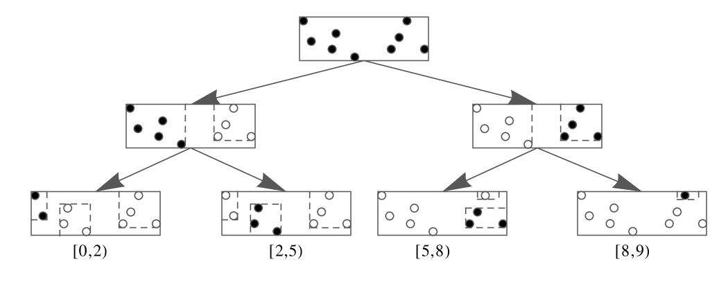
Figure 2: kd𝑘𝑑kd-tree of a two-dimensional point set. At each level, the bounding box is split in half along the widest dimension. The solid points denote the points owned by each node. At each leaf node, we can enumerate each point with its depth-first rank. The minimum depth-first rank (inclusive) and the maximum depth-first rank (exclusive) is shown for each node.

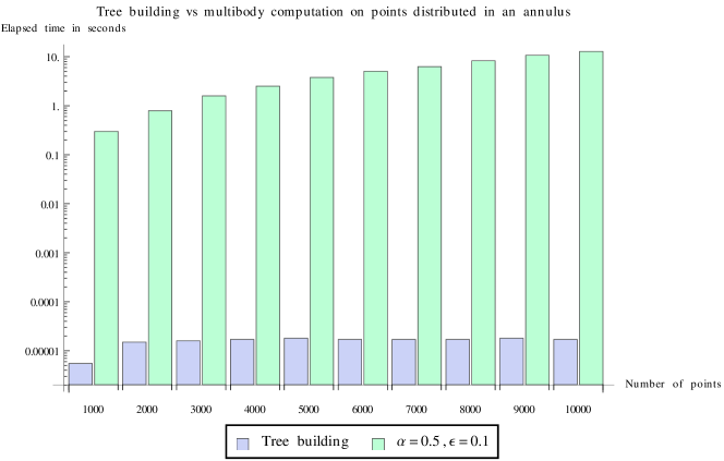
We use a variant of kd𝑘𝑑kd-trees [13] to form hierarchical groupings of points based on their locations using the recursive procedure shown in Algorithm 1. Initially, the algorithm starts with P=X𝑃𝑋P=X (the entire point set). We split a given set of points along the widest dimension of the bounding hyper-rectangle into two equal halves at the splitting coordinate. We continue splitting until the number of points is below some user-defined threshold called the leaf threshold. If the number of points owned by a node exceeds the leaf threshold, then it is called an internal node. Otherwise it is called a leaf node. Assuming that each split on a level results in the equal number of points on the left subset and the right subset PLsuperscript𝑃𝐿P^{L} and PRsuperscript𝑃𝑅P^{R} respectively, the runtime cost is 𝒪(|X|log|X|)𝒪𝑋𝑋\mathcal{O}(|X|\log|X|). We note that the cost of building a kd𝑘𝑑kd-tree is negligible compared to the actual multibody potential computation (see Section 6). See Figure 2.

Algorithm 1 BuildKdTree(P)BuildKdTree𝑃\mbox{{BuildKdTree}}(P)
  if  |P|𝑃|P| is above the leaf threshold then
     Find the widest dimension d𝑑d of the bounding box of P𝑃P.
     Choose an axis-aligned split s𝑠s along d𝑑d.
     Split P=PLPR𝑃superscript𝑃𝐿superscript𝑃𝑅P=P^{L}\cup P^{R} where PL={xP|x[d]s}superscript𝑃𝐿conditional-set𝑥𝑃𝑥delimited-[]𝑑𝑠P^{L}=\{x\in P\ |\ x[d]\leq s\} and PR=P\PLsuperscript𝑃𝑅\𝑃superscript𝑃𝐿P^{R}=P\backslash P^{L}.
     BuildKdTree(PL)BuildKdTreesuperscript𝑃𝐿\mbox{{BuildKdTree}}(P^{L}), BuildKdTree(PR)BuildKdTreesuperscript𝑃𝑅\mbox{{BuildKdTree}}(P^{R})
     Form far-field moments of P𝑃P by translating far-field moments of PLsuperscript𝑃𝐿P^{L} and PRsuperscript𝑃𝑅P^{R}.
  else
     Form far-field moments of P𝑃P.
  Initialize summary statistics of P𝑃P.

The general framework for computing Equation (1) is formalized in [5, 14, 15, 16]. This approach consists of the following steps:

  1. 1.

    Build a spatial tree (such as kd-trees) for the set of particles X𝑋X and build far-field moments on each node of the tree (Bottom-up phase).

  2. 2.

    Perform a multi-tree traversal over n𝑛n-tuples of nodes (Approximation phase).

  3. 3.

    Pre-order traverse the tree and propagate unincorporated bound changes downward (Top-down phase).

Refer to caption
Refer to caption
Figure 3: The lower and upper bound on pairwise distances between the points contained in a pair of nodes.

Step 2 utilizes the procedure shown in Algorithm 2 (called by setting each Pi=Xsubscript𝑃𝑖𝑋P_{i}=X for 1in1𝑖𝑛1\leq i\leq n), a recursive function that allows us to consider the n𝑛n-tuples formed by choosing each xisubscript𝑥𝑖x_{i} from Pisubscript𝑃𝑖P_{i}; we can gain efficiency over the naive enumeration of the n𝑛n-tuples by using the bounding box and the moment information stored in each Pisubscript𝑃𝑖P_{i}. One such information is the distance bound computed using the bounding box (see Figure 3).

Algorithm 2 MTPotentialCanonical({Pi}i=1n)MTPotentialCanonicalsuperscriptsubscriptsubscript𝑃𝑖𝑖1𝑛\mbox{{MTPotentialCanonical}}(\{P_{i}\}_{i=1}^{n})
  if CanSummarize({Pi}i=1n)CanSummarizesuperscriptsubscriptsubscript𝑃𝑖𝑖1𝑛\mbox{{CanSummarize}}(\{P_{i}\}_{i=1}^{n})    (Try approximation.) then
     Summarize({Pi}i=1n,ϵ,τ,α)Summarizesuperscriptsubscriptsubscript𝑃𝑖𝑖1𝑛italic-ϵ𝜏𝛼\mbox{{Summarize}}(\{P_{i}\}_{i=1}^{n},\epsilon,\tau,\alpha)
  else
     if all of Sisubscript𝑆𝑖S_{i} are leaves then
        MTPotentialBase({Pi}i=1n)MTPotentialBasesuperscriptsubscriptsubscript𝑃𝑖𝑖1𝑛\mbox{{MTPotentialBase}}(\{P_{i}\}_{i=1}^{n})    (Base case.)
     else
        Find an internal node Pksubscript𝑃𝑘P_{k} to split among {Pi}i=1nsuperscriptsubscriptsubscript𝑃𝑖𝑖1𝑛\{P_{i}\}_{i=1}^{n}.
        Propagate bounds of Pksubscript𝑃𝑘P_{k} to PkLsuperscriptsubscript𝑃𝑘𝐿P_{k}^{L} and PkRsuperscriptsubscript𝑃𝑘𝑅P_{k}^{R}.
        MTPotentialCanonical({P1,,Pk1,PkL,Pk+1,,Pn})MTPotentialCanonicalsubscript𝑃1subscript𝑃𝑘1superscriptsubscript𝑃𝑘𝐿subscript𝑃𝑘1subscript𝑃𝑛\mbox{{MTPotentialCanonical}}(\{P_{1},\cdots,P_{k-1},P_{k}^{L},P_{k+1},\cdots,P_{n}\})
        MTPotentialCanonical({P1,,Pk1,PkR,Pk+1,,Pn})MTPotentialCanonicalsubscript𝑃1subscript𝑃𝑘1superscriptsubscript𝑃𝑘𝑅subscript𝑃𝑘1subscript𝑃𝑛\mbox{{MTPotentialCanonical}}(\{P_{1},\cdots,P_{k-1},P_{k}^{R},P_{k+1},\cdots,P_{n}\})
        Refine summary statistics based on the two recursive calls.

CanSummarize function first eliminates redundant recursive calls for the list of node tuples that satisfy the following condition: if there exists a pair of nodes Pisubscript𝑃𝑖P_{i} and Pjsubscript𝑃𝑗P_{j} (i<j𝑖𝑗i<j) among the node list P1,,Pnsubscript𝑃1subscript𝑃𝑛P_{1},\cdots,P_{n}, such that the maximum depth-first rank of Pisubscript𝑃𝑖P_{i} is less than the minimum depth-first rank of Pjsubscript𝑃𝑗P_{j}. In this case, the function returns true. See Figure 2 and [17]. In addition, if any one of the nodes in the list includes one of the other nodes (i.e. there exists nodes Pisubscript𝑃𝑖P_{i} and Pjsubscript𝑃𝑗P_{j} such that the minimum depth-first rank of Pi<subscript𝑃𝑖absentP_{i}< the minimum depth-first rank of Pj<subscript𝑃𝑗absentP_{j}< the maximum depth-first rank of Pj<subscript𝑃𝑗absentP_{j}< the maximum depth-first rank of Pisubscript𝑃𝑖P_{i}), CanSummarize returns false. We do this because it is a bit tricky to count the number of tuples for each point in this case (see Figure 4).

Refer to caption
Refer to caption
Refer to caption
Refer to caption
Figure 4: For n=3𝑛3n=3, four canonical cases of the three “valid” (i.e. the particle indices in each node are in increasing depth-first order) node tuples encountered during the algorithm: (a) All three nodes are equal; (b) S1subscript𝑆1S_{1} and S2subscript𝑆2S_{2} are equal, and S3subscript𝑆3S_{3} comes later in the depth-first order; (c) S2subscript𝑆2S_{2} and S3subscript𝑆3S_{3} are equal and come later in the depth-first order; (d) All three nodes are different.

Otherwise, CanSummarize function tests whether each potential sum for x1mnPm𝑥subscript1𝑚𝑛subscript𝑃𝑚x\in\bigcup\limits_{1\leq m\leq n}P_{m} can be approximated within the error tolerance determined by the algorithm. For example, if n=4𝑛4n=4, we test for each x1P1subscript𝑥1subscript𝑃1x_{1}\in P_{1}, x2P2subscript𝑥2subscript𝑃2x_{2}\in P_{2}, x3P3subscript𝑥3subscript𝑃3x_{3}\in P_{3}, x4P4subscript𝑥4subscript𝑃4x_{4}\in P_{4}, the following exact quantities can be approximated:

Φ(x1;P2×P3×P4)Φsubscript𝑥1subscript𝑃2subscript𝑃3subscript𝑃4\displaystyle\Phi(x_{1};P_{2}\times P_{3}\times P_{4}) =xi2P2\{x1}xi3P3\{x1}i2<i3xi4P4\{x1}i3<i4ϕ(x1,xi2,xi3,xi4)absentsubscriptsubscript𝑥subscript𝑖2\subscript𝑃2subscript𝑥1subscriptsubscript𝑥subscript𝑖3\subscript𝑃3subscript𝑥1subscript𝑖2subscript𝑖3subscriptsubscript𝑥subscript𝑖4\subscript𝑃4subscript𝑥1subscript𝑖3subscript𝑖4italic-ϕsubscript𝑥1subscript𝑥subscript𝑖2subscript𝑥subscript𝑖3subscript𝑥subscript𝑖4\displaystyle=\sum\limits_{x_{i_{2}}\in P_{2}\backslash\{x_{1}\}}\ \sum\limits_{\begin{subarray}{c}x_{i_{3}}\in P_{3}\backslash\{x_{1}\}\\ i_{2}<i_{3}\end{subarray}}\ \sum\limits_{\begin{subarray}{c}x_{i_{4}}\in P_{4}\backslash\{x_{1}\}\\ i_{3}<i_{4}\end{subarray}}\phi(x_{1},x_{i_{2}},x_{i_{3}},x_{i_{4}})
Φ(x2;P1×P3×P4)Φsubscript𝑥2subscript𝑃1subscript𝑃3subscript𝑃4\displaystyle\Phi(x_{2};P_{1}\times P_{3}\times P_{4}) =xi1P1\{x2}xi3P3\{x2}i1<i3xi4P4\{x2}i3<i4ϕ(x2,xi1,xi3,xi4)absentsubscriptsubscript𝑥subscript𝑖1\subscript𝑃1subscript𝑥2subscriptsubscript𝑥subscript𝑖3\subscript𝑃3subscript𝑥2subscript𝑖1subscript𝑖3subscriptsubscript𝑥subscript𝑖4\subscript𝑃4subscript𝑥2subscript𝑖3subscript𝑖4italic-ϕsubscript𝑥2subscript𝑥subscript𝑖1subscript𝑥subscript𝑖3subscript𝑥subscript𝑖4\displaystyle=\sum\limits_{x_{i_{1}}\in P_{1}\backslash\{x_{2}\}}\ \sum\limits_{\begin{subarray}{c}x_{i_{3}}\in P_{3}\backslash\{x_{2}\}\\ i_{1}<i_{3}\end{subarray}}\ \sum\limits_{\begin{subarray}{c}x_{i_{4}}\in P_{4}\backslash\{x_{2}\}\\ i_{3}<i_{4}\end{subarray}}\phi(x_{2},x_{i_{1}},x_{i_{3}},x_{i_{4}})
Φ(x3;P1×P2×P4)Φsubscript𝑥3subscript𝑃1subscript𝑃2subscript𝑃4\displaystyle\Phi(x_{3};P_{1}\times P_{2}\times P_{4}) =xi1P1\{x3}xi2P2\{x3}i1<i2xi4P4\{x3}i2<i4ϕ(x3,xi1,xi2,xi4)absentsubscriptsubscript𝑥subscript𝑖1\subscript𝑃1subscript𝑥3subscriptsubscript𝑥subscript𝑖2\subscript𝑃2subscript𝑥3subscript𝑖1subscript𝑖2subscriptsubscript𝑥subscript𝑖4\subscript𝑃4subscript𝑥3subscript𝑖2subscript𝑖4italic-ϕsubscript𝑥3subscript𝑥subscript𝑖1subscript𝑥subscript𝑖2subscript𝑥subscript𝑖4\displaystyle=\sum\limits_{x_{i_{1}}\in P_{1}\backslash\{x_{3}\}}\ \sum\limits_{\begin{subarray}{c}x_{i_{2}}\in P_{2}\backslash\{x_{3}\}\\ i_{1}<i_{2}\end{subarray}}\ \sum\limits_{\begin{subarray}{c}x_{i_{4}}\in P_{4}\backslash\{x_{3}\}\\ i_{2}<i_{4}\end{subarray}}\phi(x_{3},x_{i_{1}},x_{i_{2}},x_{i_{4}})
Φ(x4;P1×P2×P3)Φsubscript𝑥4subscript𝑃1subscript𝑃2subscript𝑃3\displaystyle\Phi(x_{4};P_{1}\times P_{2}\times P_{3}) =xi1P1\{x4}xi2P2\{x4}i1<i2xi3P3\{x4}i2<i3ϕ(x4,xi1,xi2,xi3)absentsubscriptsubscript𝑥subscript𝑖1\subscript𝑃1subscript𝑥4subscriptsubscript𝑥subscript𝑖2\subscript𝑃2subscript𝑥4subscript𝑖1subscript𝑖2subscriptsubscript𝑥subscript𝑖3\subscript𝑃3subscript𝑥4subscript𝑖2subscript𝑖3italic-ϕsubscript𝑥4subscript𝑥subscript𝑖1subscript𝑥subscript𝑖2subscript𝑥subscript𝑖3\displaystyle=\sum\limits_{x_{i_{1}}\in P_{1}\backslash\{x_{4}\}}\ \sum\limits_{\begin{subarray}{c}x_{i_{2}}\in P_{2}\backslash\{x_{4}\}\\ i_{1}<i_{2}\end{subarray}}\ \sum\limits_{\begin{subarray}{c}x_{i_{3}}\in P_{3}\backslash\{x_{4}\}\\ i_{2}<i_{3}\end{subarray}}\phi(x_{4},x_{i_{1}},x_{i_{2}},x_{i_{3}})

If the approximation is not possible, then the algorithm continues to consider the data at a finer granularity; it chooses an internal node Pksubscript𝑃𝑘P_{k} (typically the one with the largest diameter) to split among {Pi}i=1nsuperscriptsubscriptsubscript𝑃𝑖𝑖1𝑛\{P_{i}\}_{i=1}^{n}. Before recursing to two sub-calls in Line 9 and Line 10 of Algorithm 2, the algorithm can optionally push quantities from a node that is being split to its child nodes (Line 8). After returning from the recursive calls, the node that was just split can refine summary statistics based on the results accumulated on its child nodes. The details of these operations are available in earlier papers [5, 14, 15, 16, 18].

The basic idea is to terminate the recursion as soon as possible, i.e. by considering a tuple of large subsets and avoiding the number of exhaustive leaf-leaf-leaf computations. We note that the CanSummarize and Summarize functions effectively replace unwieldy interaction lists used in FMM algorithms. Interaction lists in n𝑛n-tuple interaction, if naively enumerated, can be large depending on the potential function ϕitalic-ϕ\phi and the dimensionality D𝐷D of the problem, whereas the generalized N𝑁N-body approach can handle a wide spectrum of problems without this drawback.
Refer to caption
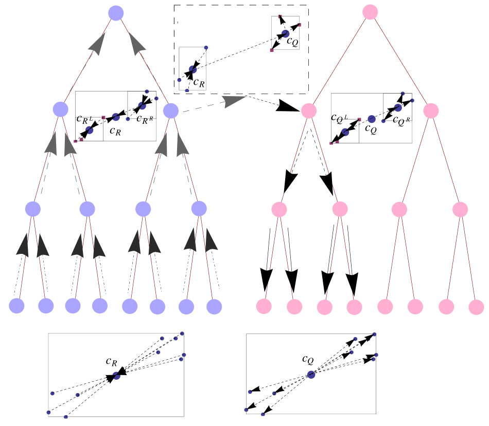
Figure 5: The reference points (the left tree) are hierarchically compressed and uncompressed when a pair of query (from the right tree)/reference nodes is approximated within an error tolerance.

3.1 Algorithm for Pairwise Potentials (n=2𝑛2n=2)

The general algorithmic strategy for pairwise potentials ϕ(,)italic-ϕ\phi(\cdot,\cdot) is described in [5, 14, 15, 16], and consists of the following three main phases (see Figure 5). Suppose we are given a set of “source” points (denoted as reference points) and a set of “target” points (denoted as query points)222The terms “reference/query” have been used in the general framework we are applying.

  1. 1.

    Bottom-up phase: Compute far-field moments of order p𝑝p in every leaf node of the reference tree. The resulting far-field expansion of each reference node P2subscript𝑃2P_{2} is given by:

    Φ(x;P2)=𝜶0[xi2P2(1)𝜶𝜶!(xi2cP2)𝜶]D𝜶ϕ(xcP2)=𝜶0M𝜶(P2,cP2)D𝜶ϕ(xcP2)Φ𝑥subscript𝑃2subscript𝜶0delimited-[]subscriptsubscript𝑥subscript𝑖2subscript𝑃2superscript1𝜶𝜶superscriptsubscript𝑥subscript𝑖2subscript𝑐subscript𝑃2𝜶superscript𝐷𝜶italic-ϕ𝑥subscript𝑐subscript𝑃2subscript𝜶0subscript𝑀𝜶subscript𝑃2subscript𝑐subscript𝑃2superscript𝐷𝜶italic-ϕ𝑥subscript𝑐subscript𝑃2\displaystyle\Phi(x;P_{2})=\sum\limits_{\bm{\alpha}\geq 0}\left[\sum\limits_{x_{i_{2}}\in P_{2}}\frac{(-1)^{\bm{\alpha}}}{\bm{\alpha}!}(x_{i_{2}}-c_{P_{2}})^{\bm{\alpha}}\right]D^{\bm{\alpha}}\phi(x-c_{P_{2}})=\sum\limits_{\bm{\alpha}\geq 0}M_{\bm{\alpha}}(P_{2},c_{P_{2}})D^{\bm{\alpha}}\phi(x-c_{P_{2}})

    Φ(x;P2)Φ𝑥subscript𝑃2\Phi(x;P_{2}) reads as “the potential sum on x𝑥x due to the contribution of P2subscript𝑃2P_{2}” and M𝜶(P2,cP2)subscript𝑀𝜶subscript𝑃2subscript𝑐subscript𝑃2M_{\bm{\alpha}}(P_{2},c_{P_{2}}) as “the 𝜶𝜶\bm{\alpha}-th far-field coefficient of P2subscript𝑃2P_{2} centered at cP2subscript𝑐subscript𝑃2c_{P_{2}}.” Because it is impossible to store an infinite number of far-field moments M𝜶(P2,cP2)subscript𝑀𝜶subscript𝑃2subscript𝑐subscript𝑃2M_{\bm{\alpha}}(P_{2},c_{P_{2}}), we truncate the Taylor expansion up to the order p𝑝p (determined either arbitrarily or by an appropriate error criterion):

    Φ~(x;P2;F(cP2,p))=|𝜶|pM𝜶(P2,cP2)D𝜶ϕ(xcP2)~Φ𝑥subscript𝑃2𝐹subscript𝑐subscript𝑃2𝑝subscript𝜶𝑝subscript𝑀𝜶subscript𝑃2subscript𝑐subscript𝑃2superscript𝐷𝜶italic-ϕ𝑥subscript𝑐subscript𝑃2\displaystyle\widetilde{\Phi}(x;P_{2};F(c_{P_{2}},p))=\sum\limits_{|\bm{\alpha}|\leq p}M_{\bm{\alpha}}(P_{2},c_{P_{2}})D^{\bm{\alpha}}\phi(x-c_{P_{2}}) (4)

    such that |Φ~(x;P2)Φ(x;P2)|~Φ𝑥subscript𝑃2Φ𝑥subscript𝑃2\left|\widetilde{\Phi}(x;P_{2})-\Phi(x;P_{2})\right| is sufficiently small. Φ~(x;P2;F(cP2,p))~Φ𝑥subscript𝑃2𝐹subscript𝑐subscript𝑃2𝑝\widetilde{\Phi}(x;P_{2};F(c_{P_{2}},p)) reads as “the approximated potential sum on x𝑥x due to the points owned by P2subscript𝑃2P_{2} using up to the p𝑝p-th order far-field expansion of P2subscript𝑃2P_{2} centered at cP2subscript𝑐subscript𝑃2c_{P_{2}}.”

    For internal reference nodes, perform the far-to-far (F2F) translation to convert the far-field moments owned by the child nodes to form the far-field moments for their common parent node P2subscript𝑃2P_{2}. For example, the far-field moments of P2Lsubscriptsuperscript𝑃𝐿2P^{L}_{2} centered at cP2Lsubscript𝑐subscriptsuperscript𝑃𝐿2c_{P^{L}_{2}} is shifted to cP2subscript𝑐subscript𝑃2c_{P_{2}} by:

    Φ~(x;P2L;F(cP2,p))=𝜸pM𝜸(P2L,cP2)(1)𝜸D𝜸ϕ(xcP2)~Φ𝑥superscriptsubscript𝑃2𝐿𝐹subscript𝑐subscript𝑃2𝑝subscript𝜸𝑝subscript𝑀𝜸superscriptsubscript𝑃2𝐿subscript𝑐subscript𝑃2superscript1𝜸superscript𝐷𝜸italic-ϕ𝑥subscript𝑐subscript𝑃2\displaystyle\widetilde{\Phi}(x;P_{2}^{L};F(c_{P_{2}},p))=\sum\limits_{\bm{\gamma}\leq p}M_{\bm{\gamma}}(P_{2}^{L},c_{P_{2}})(-1)^{\bm{\gamma}}D^{\bm{\gamma}}\phi(x-c_{P_{2}}) (5)

    where

    M𝜸(P2L,cP2)=𝜶𝜸M𝜶(P2L,cP2L)(cP2LcP2)𝜸𝜶(𝜸𝜶)!subscript𝑀𝜸superscriptsubscript𝑃2𝐿subscript𝑐subscript𝑃2subscript𝜶𝜸subscript𝑀𝜶superscriptsubscript𝑃2𝐿subscript𝑐superscriptsubscript𝑃2𝐿superscriptsubscript𝑐superscriptsubscript𝑃2𝐿subscript𝑐subscript𝑃2𝜸𝜶𝜸𝜶M_{\bm{\gamma}}(P_{2}^{L},c_{P_{2}})=\sum\limits_{\bm{\alpha}\leq\bm{\gamma}}\frac{M_{\bm{\alpha}}(P_{2}^{L},c_{P_{2}^{L}})(c_{P_{2}^{L}}-c_{P_{2}})^{\bm{\gamma}-\bm{\alpha}}}{(\bm{\gamma}-\bm{\alpha})!} (6)

    Note that there is no error incurred in each F2F translation, i.e. Φ~(x;P2L;F(cP2L,p))=Φ~(x;P2L;F(cP2,p))~Φ𝑥superscriptsubscript𝑃2𝐿𝐹subscript𝑐superscriptsubscript𝑃2𝐿𝑝~Φ𝑥superscriptsubscript𝑃2𝐿𝐹subscript𝑐subscript𝑃2𝑝\widetilde{\Phi}(x;P_{2}^{L};F(c_{P_{2}^{L}},p))=\widetilde{\Phi}(x;P_{2}^{L};F(c_{P_{2}},p)) for any query point y𝑦y from the intersection of the domains of x𝑥x for Φ~(x;P2L;F(cP2L,p))~Φ𝑥superscriptsubscript𝑃2𝐿𝐹subscript𝑐superscriptsubscript𝑃2𝐿𝑝\widetilde{\Phi}(x;P_{2}^{L};F(c_{P_{2}^{L}},p)) and Φ~(x;P2L;F(cP2,p))~Φ𝑥superscriptsubscript𝑃2𝐿𝐹subscript𝑐subscript𝑃2𝑝\widetilde{\Phi}(x;P_{2}^{L};F(c_{P_{2}},p)); the domain for which the far-field expansion remains valid depends on the error bound criterion for each potential. The far-field moments of the parent node P2subscript𝑃2P_{2} is the sum of the translated moments of its child nodes: M𝜸(P2,cP2)=𝜶𝜸M𝜶(P2L,cP2L)(cP2LcP2)𝜸𝜶(𝜸𝜶)!+M𝜶(P2R,cP2R)(cP2RcP2)𝜸𝜶(𝜸𝜶)!subscript𝑀𝜸subscript𝑃2subscript𝑐subscript𝑃2subscript𝜶𝜸subscript𝑀𝜶superscriptsubscript𝑃2𝐿subscript𝑐superscriptsubscript𝑃2𝐿superscriptsubscript𝑐superscriptsubscript𝑃2𝐿subscript𝑐subscript𝑃2𝜸𝜶𝜸𝜶subscript𝑀𝜶superscriptsubscript𝑃2𝑅subscript𝑐superscriptsubscript𝑃2𝑅superscriptsubscript𝑐superscriptsubscript𝑃2𝑅subscript𝑐subscript𝑃2𝜸𝜶𝜸𝜶M_{\bm{\gamma}}(P_{2},c_{P_{2}})=\sum\limits_{\bm{\alpha}\leq\bm{\gamma}}\frac{M_{\bm{\alpha}}(P_{2}^{L},c_{P_{2}^{L}})(c_{P_{2}^{L}}-c_{P_{2}})^{\bm{\gamma}-\bm{\alpha}}}{(\bm{\gamma}-\bm{\alpha})!}+\frac{M_{\bm{\alpha}}(P_{2}^{R},c_{P_{2}^{R}})(c_{P_{2}^{R}}-c_{P_{2}})^{\bm{\gamma}-\bm{\alpha}}}{(\bm{\gamma}-\bm{\alpha})!}

  2. 2.

    Approximation phase: For a given pair of the query and the reference nodes, determine the order of approximation and either (1) translate the far-field moments of the reference node to the local moments of the query node (2) or recurse to their subsets, if the F2L translation is more costly than the direct exhaustive method.

    Let us re-write the exact contribution of P2subscript𝑃2P_{2} to a point xP1𝑥subscript𝑃1x\in P_{1}:

    Φ(x;P2)=𝜷01𝜷!𝜶0M𝜶(P2,cP2)D𝜶+𝜷ϕ(cP1cP2)(xcP1)𝜷Φ𝑥subscript𝑃2subscript𝜷01𝜷subscript𝜶0subscript𝑀𝜶subscript𝑃2subscript𝑐subscript𝑃2superscript𝐷𝜶𝜷italic-ϕsubscript𝑐subscript𝑃1subscript𝑐subscript𝑃2superscript𝑥subscript𝑐subscript𝑃1𝜷\displaystyle\Phi(x;P_{2})=\sum\limits_{\bm{\beta}\geq 0}\frac{1}{\bm{\beta}!}\sum\limits_{\bm{\alpha}\geq 0}M_{\bm{\alpha}}(P_{2},c_{P_{2}})D^{\bm{\alpha}+\bm{\beta}}\phi(c_{P_{1}}-c_{P_{2}})(x-c_{P_{1}})^{\bm{\beta}}
    =\displaystyle= 𝜷0[xi2P21𝜷!D𝜷ϕ(cP1xi2)](xcP1)𝜷=𝜷0N𝜷(P2,cP1)(xcP1)𝜷subscript𝜷0delimited-[]subscriptsubscript𝑥subscript𝑖2subscript𝑃21𝜷superscript𝐷𝜷italic-ϕsubscript𝑐subscript𝑃1subscript𝑥subscript𝑖2superscript𝑥subscript𝑐subscript𝑃1𝜷subscript𝜷0subscript𝑁𝜷subscript𝑃2subscript𝑐subscript𝑃1superscript𝑥subscript𝑐subscript𝑃1𝜷\displaystyle\sum\limits_{\bm{\beta}\geq 0}\left[\sum\limits_{x_{i_{2}}\in P_{2}}\frac{1}{\bm{\beta}!}D^{\bm{\beta}}\phi(c_{P_{1}}-x_{i_{2}})\right](x-c_{P_{1}})^{\bm{\beta}}=\sum\limits_{\bm{\beta}\geq 0}N_{\bm{\beta}}(P_{2},c_{P_{1}})(x-c_{P_{1}})^{\bm{\beta}} (7)

    where N𝜷(P2,cP1)subscript𝑁𝜷subscript𝑃2subscript𝑐subscript𝑃1N_{\bm{\beta}}(P_{2},c_{P_{1}}) reads as “the exact local moments 333We use N𝑁N to denote the local moments because a “near-field” expansion is another widely used term for a local expansion. It avoids the potential notational confusion in the later parts of the paper. contributed by the points in P2subscript𝑃2P_{2} centered at cP1subscript𝑐subscript𝑃1c_{P_{1}}.” Truncating Equation (7) at |𝜷|p𝜷superscript𝑝|\bm{\beta}|\leq p^{\prime} for some ppsuperscript𝑝𝑝p^{\prime}\leq p yields a direct local accumulation of order p𝑝p.

    From the bottom-up phase, we know that |𝜶|p𝜶𝑝|\bm{\alpha}|\leq p. Similarly, we can store only a finite number of local moments up to the order ppsuperscript𝑝𝑝p^{\prime}\leq p and thus |𝜷|p𝜷superscript𝑝|\bm{\beta}|\leq p^{\prime}. We get the local expansion for P1subscript𝑃1P_{1} formed due to translated far-field moments of P2subscript𝑃2P_{2}:

    Φ~(x;P2;N~(cP1,p))~Φ𝑥subscript𝑃2~𝑁subscript𝑐subscript𝑃1superscript𝑝\displaystyle\widetilde{\Phi}(x;P_{2};\widetilde{N}(c_{P_{1}},p^{\prime})) =|𝜷|p[1𝜷!|𝜶|pM𝜶(P2,cP2)D𝜶+𝜷ϕ1,2(cP1cP2)](xcP1)𝜷absentsubscript𝜷superscript𝑝delimited-[]1𝜷subscript𝜶superscript𝑝subscript𝑀𝜶subscript𝑃2subscript𝑐subscript𝑃2superscript𝐷𝜶𝜷subscriptitalic-ϕ12subscript𝑐subscript𝑃1subscript𝑐subscript𝑃2superscript𝑥subscript𝑐subscript𝑃1𝜷\displaystyle=\sum\limits_{|\bm{\beta}|\leq p^{\prime}}\left[\frac{1}{\bm{\beta}!}\sum\limits_{|\bm{\alpha}|\leq p^{\prime}}M_{\bm{\alpha}}(P_{2},c_{P_{2}})D^{\bm{\alpha}+\bm{\beta}}\phi_{1,2}(c_{P_{1}}-c_{P_{2}})\right](x-c_{P_{1}})^{\bm{\beta}}
    =|𝜷|pN~𝜷(P2,cP1)(xcP1)𝜷absentsubscript𝜷superscript𝑝subscript~𝑁𝜷subscript𝑃2subscript𝑐subscript𝑃1superscript𝑥subscript𝑐subscript𝑃1𝜷\displaystyle=\sum\limits_{|\bm{\beta}|\leq p^{\prime}}\widetilde{N}_{\bm{\beta}}(P_{2},c_{P_{1}})(x-c_{P_{1}})^{\bm{\beta}} (8)

    where N~𝜷(P2,cP1)subscript~𝑁𝜷subscript𝑃2subscript𝑐subscript𝑃1\widetilde{N}_{\bm{\beta}}(P_{2},c_{P_{1}}) reads as “approximation to the exact local moments N𝜷(P2,cP1)subscript𝑁𝜷subscript𝑃2subscript𝑐subscript𝑃1N_{\bm{\beta}}(P_{2},c_{P_{1}})” and Φ~(x;P2;N~(cP1,p))~Φ𝑥subscript𝑃2~𝑁subscript𝑐subscript𝑃1superscript𝑝\widetilde{\Phi}(x;P_{2};\widetilde{N}(c_{P_{1}},p^{\prime})) as “the approximated potential sum on x𝑥x due to the points in P2subscript𝑃2P_{2} using up to the p𝑝p-th order inexact local moments centered at cP1subscript𝑐subscript𝑃1c_{P_{1}}”. The F2L translation is applied only if |Φ~(x;P2;N~(cP1,p))Φ(x;P2)|~Φ𝑥subscript𝑃2~𝑁subscript𝑐subscript𝑃1superscript𝑝Φ𝑥subscript𝑃2\left|\widetilde{\Phi}(x;P_{2};\widetilde{N}(c_{P_{1}},p^{\prime}))-\Phi(x;P_{2})\right| is sufficiently small.

  3. 3.

    Top-down phase: Propagate the local moments of each query node (i.e. pruned quantities) to its child nodes using the local-to-local (L2L) operator. Suppose we have the following local expansion for xP1𝑥subscript𝑃1x\in P_{1}:

    Φ~(x;F2L(P1)𝐷𝐿(P1);N~(cP1,pP1u))=|𝜶|pP1uN~𝜶(F2L(P1)𝐷𝐿(P1),cP1)(xi1cP1)𝜶~Φ𝑥italic-F2Lsubscript𝑃1𝐷𝐿subscript𝑃1~𝑁subscript𝑐subscript𝑃1superscriptsubscript𝑝subscript𝑃1𝑢subscript𝜶superscriptsubscript𝑝subscript𝑃1𝑢subscript~𝑁𝜶italic-F2Lsubscript𝑃1𝐷𝐿subscript𝑃1subscript𝑐subscript𝑃1superscriptsubscript𝑥subscript𝑖1subscript𝑐subscript𝑃1𝜶\widetilde{\Phi}(x;\mathit{F2L}(P_{1})\cup\mathit{DL}(P_{1});\widetilde{N}(c_{P_{1}},p_{P_{1}}^{u}))=\sum\limits_{|\bm{\alpha}|\leq p_{P_{1}}^{u}}\widetilde{N}_{\bm{\alpha}}(\mathit{F2L}(P_{1})\cup\mathit{DL}(P_{1}),c_{P_{1}})(x_{i_{1}}-c_{P_{1}})^{\bm{\alpha}}

    where pP1usuperscriptsubscript𝑝subscript𝑃1𝑢p_{P_{1}}^{u} is the maximum approximation order among (1) the F2L translations performed for P1subscript𝑃1P_{1} and all of the ancestor nodes of P1subscript𝑃1P_{1} (denoted by F2L(P1)italic-F2Lsubscript𝑃1\mathit{F2L}(P_{1})); and (2) the direct local accumulations of P1subscript𝑃1P_{1} and those passed down from all of the ancestors of P1subscript𝑃1P_{1} (denoted by 𝐷𝐿(P1)𝐷𝐿subscript𝑃1\mathit{DL}(P_{1})). Shifting the expansion to another center cP1P1superscriptsubscript𝑐subscript𝑃1subscript𝑃1c_{P_{1}}^{*}\in P_{1} is given by:

    Φ~(x;F2L(P1)𝐷𝐿(P1);N~(cP1,pP1u))~Φ𝑥italic-F2Lsubscript𝑃1𝐷𝐿subscript𝑃1~𝑁superscriptsubscript𝑐subscript𝑃1superscriptsubscript𝑝subscript𝑃1𝑢\displaystyle\widetilde{\Phi}(x;\mathit{F2L}(P_{1})\cup\mathit{DL}(P_{1});\widetilde{N}(c_{P_{1}}^{*},p_{P_{1}}^{u})) (9)
    =\displaystyle= |𝜶|pP1u[𝜷𝜶(𝜷𝜶)N~𝜷(F2L(P1)𝐷𝐿(P1),cP1)(cP1cP1)𝜷𝜶](xcP1)𝜶subscript𝜶superscriptsubscript𝑝subscript𝑃1𝑢delimited-[]subscript𝜷𝜶binomial𝜷𝜶subscript~𝑁𝜷italic-F2Lsubscript𝑃1𝐷𝐿subscript𝑃1subscript𝑐subscript𝑃1superscriptsuperscriptsubscript𝑐subscript𝑃1subscript𝑐subscript𝑃1𝜷𝜶superscript𝑥superscriptsubscript𝑐subscript𝑃1𝜶\displaystyle\sum\limits_{|\bm{\alpha}|\leq p_{P_{1}}^{u}}\left[\sum\limits_{\bm{\beta}\geq\bm{\alpha}}\binom{\bm{\beta}}{\bm{\alpha}}\widetilde{N}_{\bm{\beta}}(\mathit{F2L}(P_{1})\cup\mathit{DL}(P_{1}),c_{P_{1}})(c_{P_{1}}^{*}-c_{P_{1}})^{\bm{\beta}-\bm{\alpha}}\right](x-c_{P_{1}}^{*})^{\bm{\alpha}}
    =\displaystyle= |𝜶|pP1uN~𝜶(F2L(P1)𝐷𝐿(P1),cP1)(xcP1)𝜶subscript𝜶superscriptsubscript𝑝subscript𝑃1𝑢subscript~𝑁𝜶italic-F2Lsubscript𝑃1𝐷𝐿subscript𝑃1superscriptsubscript𝑐subscript𝑃1superscript𝑥superscriptsubscript𝑐subscript𝑃1𝜶\displaystyle\sum\limits_{|\bm{\alpha}|\leq p_{P_{1}}^{u}}\widetilde{N}_{\bm{\alpha}}(\mathit{F2L}(P_{1})\cup\mathit{DL}(P_{1}),c_{P_{1}}^{*})(x-c_{P_{1}}^{*})^{\bm{\alpha}} (10)

    This shifted moments are added to the local moments of each child of P1subscript𝑃1P_{1}, in effect transmitting the pruned contributions downward. At each query leaf, we evaluate the resulting local expansion at each query point.
Refer to caption
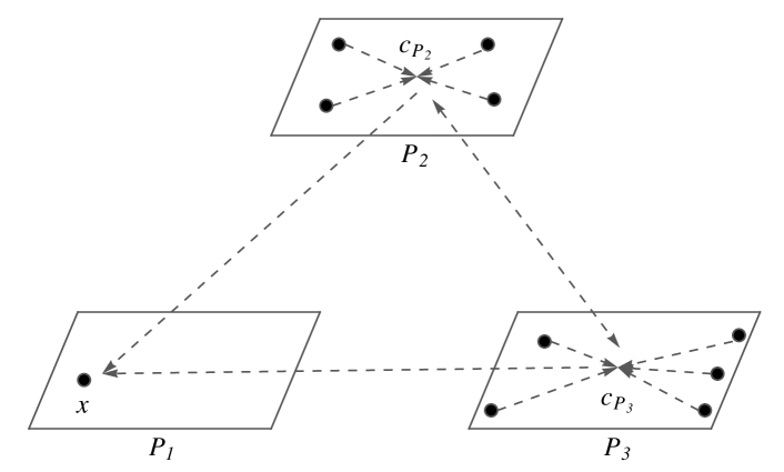
Figure 6: A far-field expansion at xi1subscript𝑥subscript𝑖1x_{i_{1}} created by the moments of P2subscript𝑃2P_{2} and P3subscript𝑃3P_{3}. Note the double-arrow between the nodes P2subscript𝑃2P_{2} and P3subscript𝑃3P_{3} corresponding to the basis functions D𝜶𝜶1,2𝜶1,3ϕ2,3(P2cP3c)superscript𝐷𝜶subscript𝜶12subscript𝜶13subscriptitalic-ϕ23superscriptsubscript𝑃2𝑐superscriptsubscript𝑃3𝑐D^{\bm{\alpha}-\bm{\alpha}_{1,2}-\bm{\alpha}_{1,3}}\phi_{2,3}(P_{2}^{c}-P_{3}^{c}) (see Equation 13).

3.2 Far-field Expansion for Three-body Potentials (n=3𝑛3n=3)

In this section, we define far-field expansions for a three-body potential that is a product of functions of pairwise distances (see Equation (1)):

ϕ(xi1,xi2,xi3)=ϕ1,2(xi1,xi2)ϕ1,3(xi1,xi3)ϕ2,3(xi2,xi3)italic-ϕsubscript𝑥subscript𝑖1subscript𝑥subscript𝑖2subscript𝑥subscript𝑖3subscriptitalic-ϕ12subscript𝑥subscript𝑖1subscript𝑥subscript𝑖2subscriptitalic-ϕ13subscript𝑥subscript𝑖1subscript𝑥subscript𝑖3subscriptitalic-ϕ23subscript𝑥subscript𝑖2subscript𝑥subscript𝑖3\phi(x_{i_{1}},x_{i_{2}},x_{i_{3}})=\phi_{1,2}(x_{i_{1}},x_{i_{2}})\cdot\phi_{1,3}(x_{i_{1}},x_{i_{3}})\cdot\phi_{2,3}(x_{i_{2}},x_{i_{3}}) (11)

We define the far-field moments of a node the same way defined for the pairwise potential case. Suppose we are given three nodes P1P2P3subscript𝑃1subscript𝑃2subscript𝑃3P_{1}\not=P_{2}\not=P_{3} from the tree. The following (n1)𝑛1(n-1)-nested sum expresses the contribution for xP1𝑥subscript𝑃1x\in P_{1} due to the other nodes P2subscript𝑃2P_{2} and P3subscript𝑃3P_{3}:

Φ(x;P2×P3)=xi2P2xi3P3ϕ(x,xi2,xi3)Φ𝑥subscript𝑃2subscript𝑃3subscriptsubscript𝑥subscript𝑖2subscript𝑃2subscriptsubscript𝑥subscript𝑖3subscript𝑃3italic-ϕ𝑥subscript𝑥subscript𝑖2subscript𝑥subscript𝑖3\Phi(x;P_{2}\times P_{3})=\sum\limits_{x_{i_{2}}\in P_{2}}\sum\limits_{x_{i_{3}}\in P_{3}}\phi(x,x_{i_{2}},x_{i_{3}}) (12)

The basic goal here is to decompose Equation (12) into sums of products of the far-field moments of each node. A far-field expansion for xi1P1subscript𝑥subscript𝑖1subscript𝑃1x_{i_{1}}\in P_{1} induced by the far-field moments of P2subscript𝑃2P_{2} and P3subscript𝑃3P_{3} is given by (see Figure 6):

Φ(x;P2×P3)Φ𝑥subscript𝑃2subscript𝑃3\displaystyle\Phi(x;P_{2}\times P_{3})
=\displaystyle= xi2P2xi3P3𝜶1,20(xi2cP2)𝜶1,2𝜶1,2!(1)𝜶1,2D𝜶1,2ϕ1,2(xcP2)subscriptsubscript𝑥subscript𝑖2subscript𝑃2subscriptsubscript𝑥subscript𝑖3subscript𝑃3subscriptsubscript𝜶120superscriptsubscript𝑥subscript𝑖2subscript𝑐subscript𝑃2subscript𝜶12subscript𝜶12superscript1subscript𝜶12superscript𝐷subscript𝜶12subscriptitalic-ϕ12𝑥subscript𝑐subscript𝑃2\displaystyle\sum\limits_{x_{i_{2}}\in P_{2}}\sum\limits_{x_{i_{3}}\in P_{3}}\sum\limits_{\bm{\alpha}_{1,2}\geq 0}\frac{(x_{i_{2}}-c_{P_{2}})^{\bm{\alpha}_{1,2}}}{\bm{\alpha}_{1,2}!}(-1)^{\bm{\alpha}_{1,2}}D^{\bm{\alpha}_{1,2}}\phi_{1,2}(x-c_{P_{2}})
𝜶1,30(xi3cP3)𝜶1,3𝜶1,3!(1)𝜶1,3D𝜶1,3ϕ1,3(xcP3)subscriptsubscript𝜶130superscriptsubscript𝑥subscript𝑖3subscript𝑐subscript𝑃3subscript𝜶13subscript𝜶13superscript1subscript𝜶13superscript𝐷subscript𝜶13subscriptitalic-ϕ13𝑥subscript𝑐subscript𝑃3\displaystyle\sum\limits_{\bm{\alpha}_{1,3}\geq 0}\frac{(x_{i_{3}}-c_{P_{3}})^{\bm{\alpha}_{1,3}}}{\bm{\alpha}_{1,3}!}(-1)^{\bm{\alpha}_{1,3}}D^{\bm{\alpha}_{1,3}}\phi_{1,3}(x-c_{P_{3}})
𝜶2,30𝜷2,3𝜶2,3(xi2cP2)𝜷2,3𝜷2,3!(xi3cP3)𝜶2,3𝜷2,3(𝜶2,3𝜷2,3)!(1)𝜶2,3𝜷2,3D𝜶2,3ϕ2,3(cP2cP3)subscriptsubscript𝜶230subscriptsubscript𝜷23subscript𝜶23superscriptsubscript𝑥subscript𝑖2subscript𝑐subscript𝑃2subscript𝜷23subscript𝜷23superscriptsubscript𝑥subscript𝑖3subscript𝑐subscript𝑃3subscript𝜶23subscript𝜷23subscript𝜶23subscript𝜷23superscript1subscript𝜶23subscript𝜷23superscript𝐷subscript𝜶23subscriptitalic-ϕ23subscript𝑐subscript𝑃2subscript𝑐subscript𝑃3\displaystyle\sum\limits_{\bm{\alpha}_{2,3}\geq 0}\sum\limits_{\bm{\beta}_{2,3}\leq\bm{\alpha}_{2,3}}\frac{(x_{i_{2}}-c_{P_{2}})^{\bm{\beta}_{2,3}}}{\bm{\beta}_{2,3}!}\frac{(x_{i_{3}}-c_{P_{3}})^{\bm{\alpha}_{2,3}-\bm{\beta}_{2,3}}}{(\bm{\alpha}_{2,3}-\bm{\beta}_{2,3})!}(-1)^{\bm{\alpha}_{2,3}-\bm{\beta}_{2,3}}D^{\bm{\alpha}_{2,3}}\phi_{2,3}(c_{P_{2}}-c_{P_{3}})

By setting 𝜶=𝜶1,2+𝜶1,3+𝜶2,3𝜶subscript𝜶12subscript𝜶13subscript𝜶23\bm{\alpha}=\bm{\alpha}_{1,2}+\bm{\alpha}_{1,3}+\bm{\alpha}_{2,3} and pushing the summations over xi2P2subscript𝑥subscript𝑖2subscript𝑃2x_{i_{2}}\in P_{2} and xi3P3subscript𝑥subscript𝑖3subscript𝑃3x_{i_{3}}\in P_{3} inside, we get:

Φ(x;P2×P3)=Φ𝑥subscript𝑃2subscript𝑃3absent\displaystyle\Phi(x;P_{2}\times P_{3})= 𝜶0𝜶1,2𝜶𝜶1,3𝜶𝜶1,2𝜷2,3𝜶𝜶1,2𝜶1,3(𝜶1,2+𝜷2,3𝜶1,2)(𝜶𝜶1,2𝜷2,3𝜶1,3)subscript𝜶0subscriptsubscript𝜶12𝜶subscriptsubscript𝜶13𝜶subscript𝜶12subscriptsubscript𝜷23𝜶subscript𝜶12subscript𝜶13binomialsubscript𝜶12subscript𝜷23subscript𝜶12binomial𝜶subscript𝜶12subscript𝜷23subscript𝜶13\displaystyle\sum\limits_{\bm{\alpha}\geq 0}\sum\limits_{\bm{\alpha}_{1,2}\leq\bm{\alpha}}\sum\limits_{\bm{\alpha}_{1,3}\leq\bm{\alpha}-\bm{\alpha}_{1,2}}\sum\limits_{\bm{\beta}_{2,3}\leq\bm{\alpha}-\bm{\alpha}_{1,2}-\bm{\alpha}_{1,3}}\binom{\bm{\alpha}_{1,2}+\bm{\beta}_{2,3}}{\bm{\alpha}_{1,2}}\binom{\bm{\alpha}-\bm{\alpha}_{1,2}-\bm{\beta}_{2,3}}{\bm{\alpha}_{1,3}}
M𝜶1,2+𝜷2,3(P2,cP2)M𝜶𝜶1,2𝜷2,3(P3,cP3)(1)𝜷2,3subscript𝑀subscript𝜶12subscript𝜷23subscript𝑃2subscript𝑐subscript𝑃2subscript𝑀𝜶subscript𝜶12subscript𝜷23subscript𝑃3subscript𝑐subscript𝑃3superscript1subscript𝜷23\displaystyle M_{\bm{\alpha}_{1,2}+\bm{\beta}_{2,3}}(P_{2},c_{P_{2}})M_{\bm{\alpha}-\bm{\alpha}_{1,2}-\bm{\beta}_{2,3}}(P_{3},c_{P_{3}})(-1)^{\bm{\beta}_{2,3}}
D𝜶1,2ϕ1,2(xi1cP2)D𝜶1,3ϕ1,3(xi1cP3)D𝜶𝜶1,2𝜶1,3ϕ2,3(cP2cP3)superscript𝐷subscript𝜶12subscriptitalic-ϕ12subscript𝑥subscript𝑖1subscript𝑐subscript𝑃2superscript𝐷subscript𝜶13subscriptitalic-ϕ13subscript𝑥subscript𝑖1subscript𝑐subscript𝑃3superscript𝐷𝜶subscript𝜶12subscript𝜶13subscriptitalic-ϕ23subscript𝑐subscript𝑃2subscript𝑐subscript𝑃3\displaystyle D^{\bm{\alpha}_{1,2}}\phi_{1,2}(x_{i_{1}}-c_{P_{2}})D^{\bm{\alpha}_{1,3}}\phi_{1,3}(x_{i_{1}}-c_{P_{3}})D^{\bm{\alpha}-\bm{\alpha}_{1,2}-\bm{\alpha}_{1,3}}\phi_{2,3}(c_{P_{2}}-c_{P_{3}}) (13)

Truncating 𝜶𝜶\bm{\alpha} at p𝑝p-th order yields:

Φ~(x;P2×P3;F(cP2×cP3,p))~Φ𝑥subscript𝑃2subscript𝑃3𝐹subscript𝑐subscript𝑃2subscript𝑐subscript𝑃3𝑝\displaystyle\widetilde{\Phi}(x;P_{2}\times P_{3};F(c_{P_{2}}\times c_{P_{3}},p))
=\displaystyle= |𝜶|p𝜶1,2𝜶𝜶1,3𝜶𝜶1,2𝜷2,3𝜶𝜶1,2𝜶1,3(𝜶1,2+𝜷2,3𝜶1,2)(𝜶𝜶1,2𝜷2,3𝜶1,3)subscript𝜶𝑝subscriptsubscript𝜶12𝜶subscriptsubscript𝜶13𝜶subscript𝜶12subscriptsubscript𝜷23𝜶subscript𝜶12subscript𝜶13binomialsubscript𝜶12subscript𝜷23subscript𝜶12binomial𝜶subscript𝜶12subscript𝜷23subscript𝜶13\displaystyle\sum\limits_{|\bm{\alpha}|\leq p}\sum\limits_{\bm{\alpha}_{1,2}\leq\bm{\alpha}}\sum\limits_{\bm{\alpha}_{1,3}\leq\bm{\alpha}-\bm{\alpha}_{1,2}}\sum\limits_{\bm{\beta}_{2,3}\leq\bm{\alpha}-\bm{\alpha}_{1,2}-\bm{\alpha}_{1,3}}\binom{\bm{\alpha}_{1,2}+\bm{\beta}_{2,3}}{\bm{\alpha}_{1,2}}\binom{\bm{\alpha}-\bm{\alpha}_{1,2}-\bm{\beta}_{2,3}}{\bm{\alpha}_{1,3}}
M𝜶1,2+𝜷2,3(P2,cP2)M𝜶𝜶1,2𝜷2,3(P3,cP3)(1)𝜷2,3subscript𝑀subscript𝜶12subscript𝜷23subscript𝑃2subscript𝑐subscript𝑃2subscript𝑀𝜶subscript𝜶12subscript𝜷23subscript𝑃3subscript𝑐subscript𝑃3superscript1subscript𝜷23\displaystyle M_{\bm{\alpha}_{1,2}+\bm{\beta}_{2,3}}(P_{2},c_{P_{2}})M_{\bm{\alpha}-\bm{\alpha}_{1,2}-\bm{\beta}_{2,3}}(P_{3},c_{P_{3}})(-1)^{\bm{\beta}_{2,3}}
D𝜶1,2ϕ1,2(xi1cP2)D𝜶1,3ϕ1,3(xi1cP3)D𝜶𝜶1,2𝜶1,3ϕ2,3(cP2cP3)superscript𝐷subscript𝜶12subscriptitalic-ϕ12subscript𝑥subscript𝑖1subscript𝑐subscript𝑃2superscript𝐷subscript𝜶13subscriptitalic-ϕ13subscript𝑥subscript𝑖1subscript𝑐subscript𝑃3superscript𝐷𝜶subscript𝜶12subscript𝜶13subscriptitalic-ϕ23subscript𝑐subscript𝑃2subscript𝑐subscript𝑃3\displaystyle D^{\bm{\alpha}_{1,2}}\phi_{1,2}(x_{i_{1}}-c_{P_{2}})D^{\bm{\alpha}_{1,3}}\phi_{1,3}(x_{i_{1}}-c_{P_{3}})D^{\bm{\alpha}-\bm{\alpha}_{1,2}-\bm{\alpha}_{1,3}}\phi_{2,3}(c_{P_{2}}-c_{P_{3}}) (14)

where Φ~(x;P2×P3;F(cP2×cP3,p))~Φ𝑥subscript𝑃2subscript𝑃3𝐹subscript𝑐subscript𝑃2subscript𝑐subscript𝑃3𝑝\widetilde{\Phi}(x;P_{2}\times P_{3};F(c_{P_{2}}\times c_{P_{3}},p)) reads as “the p𝑝p-th order far-field expansion at x𝑥x due to the moments of P2subscript𝑃2P_{2} centered at cP2subscript𝑐subscript𝑃2c_{P_{2}} and the moments of P3subscript𝑃3P_{3} centered at cP3subscript𝑐subscript𝑃3c_{P_{3}}.”

Computational Cost of Evaluating the Far-field Expansion. The first three summations over 𝜶𝜶\bm{\alpha}, 𝜶1,2subscript𝜶12\bm{\alpha}_{1,2}, 𝜶1,3subscript𝜶13\bm{\alpha}_{1,3} collectively contribute 𝒪(p3)𝒪superscript𝑝3\mathcal{O}(p^{3}) terms, and the inner summation contributing at most 𝒪(p3)𝒪superscript𝑝3\mathcal{O}(p^{3}) terms. Thus, evaluating the p𝑝p-th order far-field expansion for a three-body potential on a single point takes 𝒪(p6)𝒪superscript𝑝6\mathcal{O}\left(p^{6}\right) time.

3.3 Far-field Expansion for General Multibody Potentials (n2)𝑛2(n\geq 2)

For a general multibody potential that can be expressed as products of pairwise functions (see Equation (3)), the far-field expansion induced by the points in P2,,Pnsubscript𝑃2subscript𝑃𝑛P_{2},\cdots,P_{n} for xP1𝑥subscript𝑃1x\in P_{1} is:

Φ(x;P2××Pn)Φ𝑥subscript𝑃2subscript𝑃𝑛\displaystyle\Phi(x;P_{2}\times\cdots\times P_{n})
=\displaystyle= 2knxikPk𝜶1,k0(xikcPk)𝜶1,k𝜶1,k!(1)𝜶1,kD𝜶1,kϕ1,k(xcPk)subscriptproduct2𝑘𝑛subscriptsubscript𝑥subscript𝑖𝑘subscript𝑃𝑘subscriptsubscript𝜶1𝑘0superscriptsubscript𝑥subscript𝑖𝑘subscript𝑐subscript𝑃𝑘subscript𝜶1𝑘subscript𝜶1𝑘superscript1subscript𝜶1𝑘superscript𝐷subscript𝜶1𝑘subscriptitalic-ϕ1𝑘𝑥subscript𝑐subscript𝑃𝑘\displaystyle\prod\limits_{2\leq k\leq n}\sum\limits_{x_{i_{k}}\in P_{k}}\sum\limits_{\bm{\alpha}_{1,k}\geq 0}\frac{(x_{i_{k}}-c_{P_{k}})^{\bm{\alpha}_{1,k}}}{\bm{\alpha}_{1,k}!}(-1)^{\bm{\alpha}_{1,k}}D^{\bm{\alpha}_{1,k}}\phi_{1,k}(x-c_{P_{k}})
2s<tn𝜶s,t0𝜷s,t𝜶s,t(xiscPs)𝜷s,t𝜷s,t!(xitcPt)𝜶s,t𝜷s,t(𝜶s,t𝜷s,t)!(1)𝜶s,t𝜷s,tD𝜶s,tϕs,t(cPscPt)subscriptproduct2𝑠𝑡𝑛subscriptsubscript𝜶𝑠𝑡0subscriptsubscript𝜷𝑠𝑡subscript𝜶𝑠𝑡superscriptsubscript𝑥subscript𝑖𝑠subscript𝑐subscript𝑃𝑠subscript𝜷𝑠𝑡subscript𝜷𝑠𝑡superscriptsubscript𝑥subscript𝑖𝑡subscript𝑐subscript𝑃𝑡subscript𝜶𝑠𝑡subscript𝜷𝑠𝑡subscript𝜶𝑠𝑡subscript𝜷𝑠𝑡superscript1subscript𝜶𝑠𝑡subscript𝜷𝑠𝑡superscript𝐷subscript𝜶𝑠𝑡subscriptitalic-ϕ𝑠𝑡subscript𝑐subscript𝑃𝑠subscript𝑐subscript𝑃𝑡\displaystyle\prod\limits_{2\leq s<t\leq n}\sum\limits_{\bm{\alpha}_{s,t}\geq 0}\sum\limits_{\bm{\beta}_{s,t}\leq\bm{\alpha}_{s,t}}\frac{(x_{i_{s}}-c_{P_{s}})^{\bm{\beta}_{s,t}}}{\bm{\beta}_{s,t}!}\frac{(x_{i_{t}}-c_{P_{t}})^{\bm{\alpha}_{s,t}-\bm{\beta}_{s,t}}}{(\bm{\alpha}_{s,t}-\bm{\beta}_{s,t})!}(-1)^{\bm{\alpha}_{s,t}-\bm{\beta}_{s,t}}D^{\bm{\alpha}_{s,t}}\phi_{s,t}(c_{P_{s}}-c_{P_{t}})

Focus on grouping and multiplying monomial powers of (xikcPk)subscript𝑥subscript𝑖𝑘subscript𝑐subscript𝑃𝑘(x_{i_{k}}-c_{P_{k}}) for each 2kn2𝑘𝑛2\leq k\leq n:

(xikcPk)𝜶1,k+u=2k1(𝜶u,k𝜷u,k)+v=k+1n𝜷k,v𝜶1,k!u=2k1(𝜶u,k𝜷u,k)!v=k+1n𝜷k,v!superscriptsubscript𝑥subscript𝑖𝑘subscript𝑐subscript𝑃𝑘subscript𝜶1𝑘superscriptsubscript𝑢2𝑘1subscript𝜶𝑢𝑘subscript𝜷𝑢𝑘superscriptsubscript𝑣𝑘1𝑛subscript𝜷𝑘𝑣subscript𝜶1𝑘superscriptsubscriptproduct𝑢2𝑘1subscript𝜶𝑢𝑘subscript𝜷𝑢𝑘superscriptsubscriptproduct𝑣𝑘1𝑛subscript𝜷𝑘𝑣\displaystyle\frac{(x_{i_{k}}-c_{P_{k}})^{\bm{\alpha}_{1,k}+\sum\limits_{u=2}^{k-1}(\bm{\alpha}_{u,k}-\bm{\beta}_{u,k})+\sum\limits_{v=k+1}^{n}\bm{\beta}_{k,v}}}{\bm{\alpha}_{1,k}!\prod\limits_{u=2}^{k-1}(\bm{\alpha}_{u,k}-\bm{\beta}_{u,k})!\prod\limits_{v=k+1}^{n}\bm{\beta}_{k,v}!}

Let 𝝃k=𝜶1,k+u=2k1(𝜶u,k𝜷u,k)+v=k+1n𝜷k,vsubscript𝝃𝑘subscript𝜶1𝑘superscriptsubscript𝑢2𝑘1subscript𝜶𝑢𝑘subscript𝜷𝑢𝑘superscriptsubscript𝑣𝑘1𝑛subscript𝜷𝑘𝑣\bm{\xi}_{k}=\bm{\alpha}_{1,k}+\sum\limits_{u=2}^{k-1}(\bm{\alpha}_{u,k}-\bm{\beta}_{u,k})+\sum\limits_{v=k+1}^{n}\bm{\beta}_{k,v} and bk=𝝃k!𝜶1,k!u=2k1(𝜶u,k𝜷u,k)!v=k+1n𝜷k,v!subscript𝑏𝑘subscript𝝃𝑘subscript𝜶1𝑘superscriptsubscriptproduct𝑢2𝑘1subscript𝜶𝑢𝑘subscript𝜷𝑢𝑘superscriptsubscriptproduct𝑣𝑘1𝑛subscript𝜷𝑘𝑣b_{k}=\frac{\bm{\xi}_{k}!}{\bm{\alpha}_{1,k}!\prod\limits_{u=2}^{k-1}(\bm{\alpha}_{u,k}-\bm{\beta}_{u,k})!\prod\limits_{v=k+1}^{n}\bm{\beta}_{k,v}!}. Then,

Φ(x;P2××Pn)Φ𝑥subscript𝑃2subscript𝑃𝑛\displaystyle\Phi(x;P_{2}\times\cdots\times P_{n})
=\displaystyle= 2s<tn2kn𝜶1,k0𝜶s,t0𝜷s,t𝜶s,tbkM𝝃k(Pk,cPk)(1)𝜷s,tD𝜶1,kϕ1,k(xcPk)D𝜶s,tϕs,t(cPscPt)subscriptproduct2𝑠𝑡𝑛subscriptproduct2𝑘𝑛subscriptsubscript𝜶1𝑘0subscriptsubscript𝜶𝑠𝑡0subscriptsubscript𝜷𝑠𝑡subscript𝜶𝑠𝑡subscript𝑏𝑘subscript𝑀subscript𝝃𝑘subscript𝑃𝑘subscript𝑐subscript𝑃𝑘superscript1subscript𝜷𝑠𝑡superscript𝐷subscript𝜶1𝑘subscriptitalic-ϕ1𝑘𝑥subscript𝑐subscript𝑃𝑘superscript𝐷subscript𝜶𝑠𝑡subscriptitalic-ϕ𝑠𝑡subscript𝑐subscript𝑃𝑠subscript𝑐subscript𝑃𝑡\displaystyle\prod\limits_{2\leq s<t\leq n}\prod\limits_{2\leq k\leq n}\sum\limits_{\bm{\alpha}_{1,k}\geq 0}\sum\limits_{\bm{\alpha}_{s,t}\geq 0}\sum\limits_{\bm{\beta}_{s,t}\leq\bm{\alpha}_{s,t}}b_{k}\ M_{\bm{\xi}_{k}}(P_{k},c_{P_{k}})\ (-1)^{\bm{\beta}_{s,t}}\ D^{\bm{\alpha}_{1,k}}\phi_{1,k}(x-c_{P_{k}})D^{\bm{\alpha}_{s,t}}\phi_{s,t}(c_{P_{s}}-c_{P_{t}}) (15)

Equation (15) is a convolution of far-field moments of P2,,Pnsubscript𝑃2subscript𝑃𝑛P_{2},\cdots,P_{n}. We can truncate the expansion above for terms for |𝜶|=|1r<snαr,s|>p𝜶subscript1𝑟𝑠𝑛subscript𝛼𝑟𝑠𝑝|\bm{\alpha}|=\left|\sum\limits_{1\leq r<s\leq n}\alpha_{r,s}\right|>p for some p>0𝑝0p>0. Note that Equation (15) includes the n=2𝑛2n=2 and n=3𝑛3n=3 cases.

Φ~(x;P2××Pn;F(cP2××cPn,p))~Φ𝑥subscript𝑃2subscript𝑃𝑛𝐹subscript𝑐subscript𝑃2subscript𝑐subscript𝑃𝑛𝑝\displaystyle\widetilde{\Phi}(x;P_{2}\times\cdots\times P_{n};F(c_{P_{2}}\times\cdots\times c_{P_{n}},p))
=\displaystyle= 2s<tn2kn|𝜶|p𝜶1,k0𝜶s,t0𝜷s,t𝜶s,tbkM𝝃k(Pk,cPk)(1)𝜷s,tsubscriptproduct2𝑠𝑡𝑛subscriptproduct2𝑘𝑛subscript𝜶𝑝subscriptsubscript𝜶1𝑘0subscriptsubscript𝜶𝑠𝑡0subscriptsubscript𝜷𝑠𝑡subscript𝜶𝑠𝑡subscript𝑏𝑘subscript𝑀subscript𝝃𝑘subscript𝑃𝑘subscript𝑐subscript𝑃𝑘superscript1subscript𝜷𝑠𝑡\displaystyle\prod\limits_{2\leq s<t\leq n}\prod\limits_{2\leq k\leq n}\sum\limits_{|\bm{\alpha}|\leq p}\sum\limits_{\bm{\alpha}_{1,k}\geq 0}\sum\limits_{\bm{\alpha}_{s,t}\geq 0}\sum\limits_{\bm{\beta}_{s,t}\leq\bm{\alpha}_{s,t}}b_{k}\ M_{\bm{\xi}_{k}}(P_{k},c_{P_{k}})\ (-1)^{\bm{\beta}_{s,t}}
D𝜶1,kϕ1,k(xcPk)D𝜶s,tϕs,t(cPscPt)superscript𝐷subscript𝜶1𝑘subscriptitalic-ϕ1𝑘𝑥subscript𝑐subscript𝑃𝑘superscript𝐷subscript𝜶𝑠𝑡subscriptitalic-ϕ𝑠𝑡subscript𝑐subscript𝑃𝑠subscript𝑐subscript𝑃𝑡\displaystyle D^{\bm{\alpha}_{1,k}}\phi_{1,k}(x-c_{P_{k}})D^{\bm{\alpha}_{s,t}}\phi_{s,t}(c_{P_{s}}-c_{P_{t}}) (16)

Computational Cost of Evaluating the Far-field Expansion. The summations over 𝜶r,ssubscript𝜶𝑟𝑠\bm{\alpha}_{r,s} for 1r<sn1𝑟𝑠𝑛1\leq r<s\leq n collectively contribute 𝒪(p3)𝒪superscript𝑝3\mathcal{O}(p^{3}) terms, and each inner summation over 𝜷s,tsubscript𝜷𝑠𝑡\bm{\beta}_{s,t} contributing at most 𝒪(p3)𝒪superscript𝑝3\mathcal{O}(p^{3}) terms. Thus, evaluating the p𝑝p-th order far-field expansion for a general multibody potential of the form Equation (3) on a single point takes 𝒪(p3((n12)+1))𝒪superscript𝑝3binomial𝑛121\mathcal{O}\left(p^{3\left(\binom{n-1}{2}+1\right)}\right) time. In practice, we are forced to use p=0𝑝0p=0 for n>2𝑛2n>2 unless most ϕp,q(xip,xiq)subscriptitalic-ϕ𝑝𝑞subscript𝑥subscript𝑖𝑝subscript𝑥subscript𝑖𝑞\phi_{p,q}(x_{i_{p}},x_{i_{q}})’s in Equation (3) are constant functions.
Refer to caption
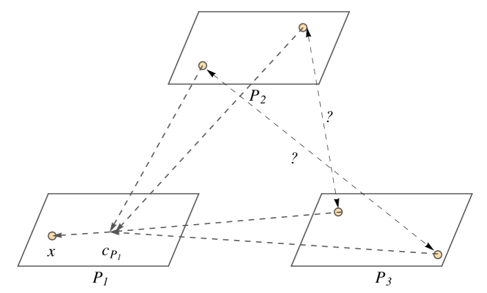
Figure 7: A local expansion created inside the node P1subscript𝑃1P_{1} at x𝑥x by directly accumulating each point in P2subscript𝑃2P_{2} and P3subscript𝑃3P_{3} (see Equation (17)). We are not aware of a technique to express an interaction between a particle in P2subscript𝑃2P_{2} and a particle in P3subscript𝑃3P_{3} (marked by the ??? symbol) for p>0𝑝0p>0.

3.4 Local Expansion for Three-body Potentials (n=3𝑛3n=3)

Unlike the far-field expansion case, we are presented a fundamental difficulty. In order to derive a local expansion, we need to express the influence of each non-evaluation point xijsubscript𝑥subscript𝑖𝑗x_{i_{j}} on the evaluation point x𝑥x at a center near x𝑥x. However, breaking up the interaction among the non-evaluation points (i.e. xijsubscript𝑥subscript𝑖𝑗x_{i_{j}}’s in the arguments of ϕ(x,xi1,,xin1)italic-ϕ𝑥subscript𝑥subscript𝑖1subscript𝑥subscript𝑖𝑛1\phi(x,x_{i_{1}},\cdots,x_{i_{n-1}})) without loss of information is hard. To see this: take a three-body potential expressible in products of pairwise functions (see Figure 7). Expanding near cP1subscript𝑐subscript𝑃1c_{P_{1}} inside the node P1subscript𝑃1P_{1} yields an expansion valid for xP1𝑥subscript𝑃1x\in P_{1}:

Φ(x;P2×P3)Φ𝑥subscript𝑃2subscript𝑃3\displaystyle\Phi(x;P_{2}\times P_{3})
=\displaystyle= xi2P2xi3P3𝜶1,20D𝜶1,2ϕ1,2(cP1xi2)𝜶1,2!(xcP1)𝜶1,2𝜶1,30D𝜶1,3ϕ1,3(cP1xi3)𝜶1,3!(xcP1)𝜶1,3subscriptsubscript𝑥subscript𝑖2subscript𝑃2subscriptsubscript𝑥subscript𝑖3subscript𝑃3subscriptsubscript𝜶120superscript𝐷subscript𝜶12subscriptitalic-ϕ12subscript𝑐subscript𝑃1subscript𝑥subscript𝑖2subscript𝜶12superscript𝑥subscript𝑐subscript𝑃1subscript𝜶12subscriptsubscript𝜶130superscript𝐷subscript𝜶13subscriptitalic-ϕ13subscript𝑐subscript𝑃1subscript𝑥subscript𝑖3subscript𝜶13superscript𝑥subscript𝑐subscript𝑃1subscript𝜶13\displaystyle\sum\limits_{x_{i_{2}}\in P_{2}}\sum\limits_{x_{i_{3}}\in P_{3}}\sum\limits_{\bm{\alpha}_{1,2}\geq 0}\frac{D^{\bm{\alpha}_{1,2}}\phi_{1,2}(c_{P_{1}}-x_{i_{2}})}{\bm{\alpha}_{1,2}!}(x-c_{P_{1}})^{\bm{\alpha}_{1,2}}\sum\limits_{\bm{\alpha}_{1,3}\geq 0}\frac{D^{\bm{\alpha}_{1,3}}\phi_{1,3}(c_{P_{1}}-x_{i_{3}})}{\bm{\alpha}_{1,3}!}(x-c_{P_{1}})^{\bm{\alpha}_{1,3}}
𝜶2,30D𝜶2,3ϕ2,3(cP1xi3)𝜶2,3!(xi2cP1)𝜶2,3subscriptsubscript𝜶230superscript𝐷subscript𝜶23subscriptitalic-ϕ23subscript𝑐subscript𝑃1subscript𝑥subscript𝑖3subscript𝜶23superscriptsubscript𝑥subscript𝑖2subscript𝑐subscript𝑃1subscript𝜶23\displaystyle\sum\limits_{\bm{\alpha}_{2,3}\geq 0}\frac{D^{\bm{\alpha}_{2,3}}\phi_{2,3}(c_{P_{1}}-x_{i_{3}})}{\bm{\alpha}_{2,3}!}(x_{i_{2}}-c_{P_{1}})^{\bm{\alpha}_{2,3}}

Again, let 𝜶=𝜶1,2+𝜶1,3+𝜶2,3𝜶subscript𝜶12subscript𝜶13subscript𝜶23\bm{\alpha}=\bm{\alpha}_{1,2}+\bm{\alpha}_{1,3}+\bm{\alpha}_{2,3}. Switching the orders of summations results:

Φ(x;P2×P3)=Φ𝑥subscript𝑃2subscript𝑃3absent\displaystyle\Phi(x;P_{2}\times P_{3})= 𝜶0𝜶1,2𝜶𝜶1,3𝜶𝜶1,2[xi2P2D𝜶1,2ϕ1,2(cP1xi2)𝜶1,2!(xi2cP1)𝜶2,3]subscript𝜶0subscriptsubscript𝜶12𝜶subscriptsubscript𝜶13𝜶subscript𝜶12delimited-[]subscriptsubscript𝑥subscript𝑖2subscript𝑃2superscript𝐷subscript𝜶12subscriptitalic-ϕ12subscript𝑐subscript𝑃1subscript𝑥subscript𝑖2subscript𝜶12superscriptsubscript𝑥subscript𝑖2subscript𝑐subscript𝑃1subscript𝜶23\displaystyle\sum\limits_{\bm{\alpha}\geq 0}\ \sum\limits_{\bm{\alpha}_{1,2}\leq\bm{\alpha}}\ \sum\limits_{\bm{\alpha}_{1,3}\leq\bm{\alpha}-\bm{\alpha}_{1,2}}\left[\sum\limits_{x_{i_{2}}\in P_{2}}\frac{D^{\bm{\alpha}_{1,2}}\phi_{1,2}(c_{P_{1}}-x_{i_{2}})}{\bm{\alpha}_{1,2}!}(x_{i_{2}}-c_{P_{1}})^{\bm{\alpha}_{2,3}}\right]
[xi3P3D𝜶1,3ϕ1,3(cP1xi3)𝜶1,3!D𝜶2,3ϕ2,3(cP1xi3)𝜶2,3!](xcP1)𝜶1,2+𝜶1,3delimited-[]subscriptsubscript𝑥subscript𝑖3subscript𝑃3superscript𝐷subscript𝜶13subscriptitalic-ϕ13subscript𝑐subscript𝑃1subscript𝑥subscript𝑖3subscript𝜶13superscript𝐷subscript𝜶23subscriptitalic-ϕ23subscript𝑐subscript𝑃1subscript𝑥subscript𝑖3subscript𝜶23superscript𝑥subscript𝑐subscript𝑃1subscript𝜶12subscript𝜶13\displaystyle\left[\sum\limits_{x_{i_{3}}\in P_{3}}\frac{D^{\bm{\alpha}_{1,3}}\phi_{1,3}(c_{P_{1}}-x_{i_{3}})}{\bm{\alpha}_{1,3}!}\frac{D^{\bm{\alpha}_{2,3}}\phi_{2,3}(c_{P_{1}}-x_{i_{3}})}{\bm{\alpha}_{2,3}!}\right](x-c_{P_{1}})^{\bm{\alpha}_{1,2}+\bm{\alpha}_{1,3}}
=\displaystyle= 𝜶0[𝜶1,2𝜶𝜶1,3𝜶𝜶1,2N¯𝜶(P2,cP1)N¯𝜶(P3,cP1)](xcP1)𝜶1,2+𝜶1,3subscript𝜶0delimited-[]subscriptsubscript𝜶12𝜶subscriptsubscript𝜶13𝜶subscript𝜶12subscript¯𝑁𝜶subscript𝑃2subscript𝑐subscript𝑃1subscript¯𝑁𝜶subscript𝑃3subscript𝑐subscript𝑃1superscript𝑥subscript𝑐subscript𝑃1subscript𝜶12subscript𝜶13\displaystyle\sum\limits_{\bm{\alpha}\geq 0}\left[\sum\limits_{\bm{\alpha}_{1,2}\leq\bm{\alpha}}\ \sum\limits_{\bm{\alpha}_{1,3}\leq\bm{\alpha}-\bm{\alpha}_{1,2}}\bar{N}_{\bm{\alpha}}(P_{2},c_{P_{1}})\ \bar{N}_{\bm{\alpha}}(P_{3},c_{P_{1}})\right](x-c_{P_{1}})^{\bm{\alpha}_{1,2}+\bm{\alpha}_{1,3}} (17)

We need the exponent of (xcP1)𝑥subscript𝑐subscript𝑃1(x-c_{P_{1}}) to match α𝛼\alpha to be able to define the local moments inside P1subscript𝑃1P_{1}. Unless α2,3=0subscript𝛼230\alpha_{2,3}=0 (i.e. ignore the interaction between a particle in the second set and a particle in the third set), this is not possible. Since we encounter a similar problem in the general case, we will skip its discussion.

4 Simpler Algorithm for General Multibody Potentials

Instead of trying to derive the full-fledged tools for general multibody potentials, we focus on deriving something simpler. Let us focus on the n=3𝑛3n=3 case. For a given set of three pairwise disjoint nodes: P1subscript𝑃1P_{1}, P2subscript𝑃2P_{2}, P3subscript𝑃3P_{3} and a monotonically decreasing444“Monotonic” multibody potentials decrease in value if one of the Euclidean distance arguments is increased while the other two are held constant. three-body potentials such as ϕ(x1,x2,x3)=1x1x2ν1,2x1x3ν1,3x2x3ν2,3italic-ϕsubscript𝑥1subscript𝑥2subscript𝑥31superscriptnormsubscript𝑥1subscript𝑥2subscript𝜈12superscriptnormsubscript𝑥1subscript𝑥3subscript𝜈13superscriptnormsubscript𝑥2subscript𝑥3subscript𝜈23\phi(x_{1},x_{2},x_{3})=\frac{1}{||x_{1}-x_{2}||^{\nu_{1,2}}||x_{1}-x_{3}||^{\nu_{1,3}}||x_{2}-x_{3}||^{\nu_{2,3}}},

xiP1,for-allsubscript𝑥𝑖subscript𝑃1\displaystyle\forall x_{i}\in P_{1}, Φ~(xi;P2×P3)=|P2||P3|ϕ(cP1,cP2,cP3)~Φsubscript𝑥𝑖subscript𝑃2subscript𝑃3subscript𝑃2subscript𝑃3italic-ϕsubscript𝑐subscript𝑃1subscript𝑐subscript𝑃2subscript𝑐subscript𝑃3\displaystyle\widetilde{\Phi}(x_{i};P_{2}\times P_{3})=|P_{2}||P_{3}|\phi(c_{P_{1}},c_{P_{2}},c_{P_{3}})
xjP2,for-allsubscript𝑥𝑗subscript𝑃2\displaystyle\forall x_{j}\in P_{2}, Φ~(xj;P1×P3)=|P1||P3|ϕ(cP1,cP2,cP3)~Φsubscript𝑥𝑗subscript𝑃1subscript𝑃3subscript𝑃1subscript𝑃3italic-ϕsubscript𝑐subscript𝑃1subscript𝑐subscript𝑃2subscript𝑐subscript𝑃3\displaystyle\widetilde{\Phi}(x_{j};P_{1}\times P_{3})=|P_{1}||P_{3}|\phi(c_{P_{1}},c_{P_{2}},c_{P_{3}})
xkP3,for-allsubscript𝑥𝑘subscript𝑃3\displaystyle\forall x_{k}\in P_{3}, Φ~(xk;P1×P2)=|P1||P2|ϕ(cP1,cP2,cP3)~Φsubscript𝑥𝑘subscript𝑃1subscript𝑃2subscript𝑃1subscript𝑃2italic-ϕsubscript𝑐subscript𝑃1subscript𝑐subscript𝑃2subscript𝑐subscript𝑃3\displaystyle\widetilde{\Phi}(x_{k};P_{1}\times P_{2})=|P_{1}||P_{2}|\phi(c_{P_{1}},c_{P_{2}},c_{P_{3}})

which can be obtained by setting p=0𝑝0p=0 in Equation (14). This means that we can get a cheaper approximation using the number of points owned by each node. Using the pairwise minimum and maximum node distances yields:

ϕ(du(P1,P2),du(P1,P3),du(P2,P3))ϕ(cP1,cP2,cP3)ϕ(dl(P1,P2),dl(P1,P3),dl(P2,P3))italic-ϕsuperscript𝑑𝑢subscript𝑃1subscript𝑃2superscript𝑑𝑢subscript𝑃1subscript𝑃3superscript𝑑𝑢subscript𝑃2subscript𝑃3italic-ϕsubscript𝑐subscript𝑃1subscript𝑐subscript𝑃2subscript𝑐subscript𝑃3italic-ϕsuperscript𝑑𝑙subscript𝑃1subscript𝑃2superscript𝑑𝑙subscript𝑃1subscript𝑃3superscript𝑑𝑙subscript𝑃2subscript𝑃3\displaystyle\phi(d^{u}(P_{1},P_{2}),d^{u}(P_{1},P_{3}),d^{u}(P_{2},P_{3}))\leq\phi(c_{P_{1}},c_{P_{2}},c_{P_{3}})\leq\phi(d^{l}(P_{1},P_{2}),d^{l}(P_{1},P_{3}),d^{l}(P_{2},P_{3}))

It is straightforward to generalize this for the n2𝑛2n\geq 2 case.

Non-monotonic Potentials: For non-monotonic potentials such as the Lennard-Jones potential ϕ(x1,x2)=ar12br6italic-ϕsubscript𝑥1subscript𝑥2𝑎superscript𝑟12𝑏superscript𝑟6\phi(x_{1},x_{2})=\frac{a}{r^{12}}-\frac{b}{r^{6}}, we can compute the critical points of ϕitalic-ϕ\phi and determine the intervals of monotonicity of ϕitalic-ϕ\phi and consider how ϕitalic-ϕ\phi behaves in the distance bound range between dl(P1,P2)superscript𝑑𝑙subscript𝑃1subscript𝑃2d^{l}(P_{1},P_{2}) and du(P1,P2)superscript𝑑𝑢subscript𝑃1subscript𝑃2d^{u}(P_{1},P_{2}). We take a simpler approach that results in an algorithm that is easier to code; we break up the potential into two parts such that ϕ(x1,x2,,xn)=ϕ+(x1,x2,,xn)ϕ(x1,x2,,xn)italic-ϕsubscript𝑥1subscript𝑥2subscript𝑥𝑛superscriptitalic-ϕsubscript𝑥1subscript𝑥2subscript𝑥𝑛superscriptitalic-ϕsubscript𝑥1subscript𝑥2subscript𝑥𝑛\phi(x_{1},x_{2},\cdots,x_{n})=\phi^{+}(x_{1},x_{2},\cdots,x_{n})-\phi^{-}(x_{1},x_{2},\cdots,x_{n}), and get a lower and upper bound (though a looser bound) on the contributions from the positive potential ϕ+superscriptitalic-ϕ\phi^{+} and negative potential ϕsuperscriptitalic-ϕ\phi^{-}.

4.1 Specifying the Approximation Rules

The overall algorithm which also subsumes the pairwise potential case (n=2𝑛2n=2) was shown in Algorithm 2. We can now specify the CanSummarize function for the general multibody case. For guaranteeing τ𝜏\tau absolute error bound criterion (Definition 2.1), the CanSummarize function returns true if:

|ϕ(du(P1,P2),,du(Pn1,Pn))ϕ(dl(P1,P2),,dl(Pn1,Pn))|τT𝑟𝑜𝑜𝑡italic-ϕsuperscript𝑑𝑢subscript𝑃1subscript𝑃2superscript𝑑𝑢subscript𝑃𝑛1subscript𝑃𝑛italic-ϕsuperscript𝑑𝑙subscript𝑃1subscript𝑃2superscript𝑑𝑙subscript𝑃𝑛1subscript𝑃𝑛𝜏superscript𝑇𝑟𝑜𝑜𝑡\left|\phi(d^{u}(P_{1},P_{2}),\cdots,d^{u}(P_{n-1},P_{n}))-\phi(d^{l}(P_{1},P_{2}),\cdots,d^{l}(P_{n-1},P_{n}))\right|\leq\frac{\tau}{T^{\mathit{root}}}

where Troot=(N1n1)superscript𝑇𝑟𝑜𝑜𝑡binomial𝑁1𝑛1T^{root}=\binom{N-1}{n-1} (i.e. the total number of tuples in each slice in Figure 1). Let us also define Tisubscript𝑇𝑖T_{i} to be the number of tuples containing a fixed particle in Pisubscript𝑃𝑖P_{i} (see Figure 4). For example, for n=3𝑛3n=3, the corresponding Summarize function would accumulate for each node:
for P1subscript𝑃1P_{1}: |P2||P3|ϕ(cP1,cP2,cP3)subscript𝑃2subscript𝑃3italic-ϕsubscript𝑐subscript𝑃1subscript𝑐subscript𝑃2subscript𝑐subscript𝑃3|P_{2}||P_{3}|\phi(c_{P_{1}},c_{P_{2}},c_{P_{3}}), for P2subscript𝑃2P_{2}: |P1||P3|ϕ(cP1,cP2,cP3)subscript𝑃1subscript𝑃3italic-ϕsubscript𝑐subscript𝑃1subscript𝑐subscript𝑃2subscript𝑐subscript𝑃3|P_{1}||P_{3}|\phi(c_{P_{1}},c_{P_{2}},c_{P_{3}}), and for P3subscript𝑃3P_{3}: |P1||P2|ϕ(cP1,cP2,cP3)subscript𝑃1subscript𝑃2italic-ϕsubscript𝑐subscript𝑃1subscript𝑐subscript𝑃2subscript𝑐subscript𝑃3|P_{1}||P_{2}|\phi(c_{P_{1}},c_{P_{2}},c_{P_{3}}).

Hybrid Absolute/Relative Error Guarantee. The algorithm for guaranteeing the hybrid absolute/relative error bound (Definition 2.2) deterministically (α=0𝛼0\alpha=0) is not so much different from that for guaranteeing the absolute error bound. In each node P𝑃P, we maintain the lower bound on the accumulated potentials for the particles in P𝑃P (denoted as Φl(P)superscriptΦ𝑙𝑃\Phi^{l}(P), a summary statistic stored in P𝑃P). The function CanSummarize returns true if,

|ϕ(du(P1,P2),,du(Pn1,Pn))ϕ(dl(P1,P2),,dl(Pn1,Pn))|italic-ϕsuperscript𝑑𝑢subscript𝑃1subscript𝑃2superscript𝑑𝑢subscript𝑃𝑛1subscript𝑃𝑛italic-ϕsuperscript𝑑𝑙subscript𝑃1subscript𝑃2superscript𝑑𝑙subscript𝑃𝑛1subscript𝑃𝑛\displaystyle\left|\phi(d^{u}(P_{1},P_{2}),\cdots,d^{u}(P_{n-1},P_{n}))-\phi(d^{l}(P_{1},P_{2}),\cdots,d^{l}(P_{n-1},P_{n}))\right|
\displaystyle\leq ϵmin1in(Φl(Pi)+δl(Pi;P1××Pi1×Pi+1××Pn))+τT𝑟𝑜𝑜𝑡italic-ϵsubscript1𝑖𝑛superscriptΦ𝑙subscript𝑃𝑖superscript𝛿𝑙subscript𝑃𝑖subscript𝑃1subscript𝑃𝑖1subscript𝑃𝑖1subscript𝑃𝑛𝜏superscript𝑇𝑟𝑜𝑜𝑡\displaystyle\frac{\epsilon\min\limits_{1\leq i\leq n}(\Phi^{l}(P_{i})+\delta^{l}(P_{i};P_{1}\times\cdots\times P_{i-1}\times P_{i+1}\times\cdots\times P_{n}))+\tau}{T^{\mathit{root}}} (18)

where each δl(Pi;P1××Pi1×Pi+1××Pn)=1jn,ji|Pj|ϕ(du(P1,P2),,du(Pn1,Pn))superscript𝛿𝑙subscript𝑃𝑖subscript𝑃1subscript𝑃𝑖1subscript𝑃𝑖1subscript𝑃𝑛subscriptproductformulae-sequence1𝑗𝑛𝑗𝑖subscript𝑃𝑗italic-ϕsuperscript𝑑𝑢subscript𝑃1subscript𝑃2superscript𝑑𝑢subscript𝑃𝑛1subscript𝑃𝑛\delta^{l}(P_{i};P_{1}\times\cdots\times P_{i-1}\times P_{i+1}\times\cdots\times P_{n})=\prod\limits_{1\leq j\leq n,j\neq i}|P_{j}|\phi(d^{u}(P_{1},P_{2}),\cdots,d^{u}(P_{n-1},P_{n})) (which is computed just using the contribution of the other nodes on the i𝑖i-th node) is added to the currently running lower bound on each node Φl(Pi)superscriptΦ𝑙subscript𝑃𝑖\Phi^{l}(P_{i}) to reflect the most recently available information on the lower bound. Φl(Pi)superscriptΦ𝑙subscript𝑃𝑖\Phi^{l}(P_{i}) can be incremented and tightened as the computation progresses, either in the base case or when the recursive sub-calls in Algorithm 2 are completed (Line 11).

Refer to caption
Figure 8: Three-body multipole methods for p=0𝑝0p=0 in a nutshell.

Monte Carlo-based Approximations. The error bounds provided by the bounding boxes (see Figure 3) assume that all pairs of points selected between the two nodes are collapsed to two positions that achieve the minimum distance (and vice versa for the maximum distance); therefore, these bounds are very pessimistic and loose. Here we introduce a method for approximating the potential sums with a probabilistic bound satisfying Definition 2.3. We can trade determinism for further gain in efficiency. We have an additional parameter α𝛼\alpha that controls the probability level at which the deviation between each approximation and its corresponding exact values holds. This was introduced first in [19, 20] for probabilistic approximations of aggregate sums and later extended in [21] to handle per-particle quantities. The theorem that we rely on for probabilistic approximation is the following:

Theorem 4.4.

Central limit theorem: Let f1subscript𝑓1f_{1}, f2subscript𝑓2f_{2}, \cdots, fmsubscript𝑓𝑚f_{m} be independent, identically distributed samples from the probability distribution F𝐹F with variance σ2superscript𝜎2\sigma^{2}, and μ~=1ms=1mfs~𝜇1𝑚superscriptsubscript𝑠1𝑚subscript𝑓𝑠\widetilde{\mu}=\frac{1}{m}\sum\limits_{s=1}^{m}f_{s} be the sample mean of the samples. As m𝑚m\rightarrow\infty, μ~N(μ,σ2/m)leads-to~𝜇𝑁𝜇superscript𝜎2𝑚\widetilde{\mu}\leadsto N(\mu,\sigma^{2}/m).

A widely accepted statistical rule of thumb asserts that 30 or more samples are usually enough to put a sample mean into the asymptotic regime. Berry-Esseen theorem characterizes the rate at which this convergence to normality takes place more precisely:

Algorithm 3 CanSummarize({Pi}i=1n)CanSummarizesuperscriptsubscriptsubscript𝑃𝑖𝑖1𝑛\mbox{{CanSummarize}}(\{P_{i}\}_{i=1}^{n}): the Monte Carlo-based approximation.
  if ζm𝑙𝑖𝑚𝑖𝑡min{T1,T2,T3}𝜁subscript𝑚𝑙𝑖𝑚𝑖𝑡subscript𝑇1subscript𝑇2subscript𝑇3\zeta\cdot m_{\mathit{limit}}\leq\min\{T_{1},T_{2},T_{3}\} then
     for each Pi{Pi}i=1nsubscript𝑃𝑖superscriptsubscriptsubscript𝑃𝑖𝑖1𝑛P_{i}\in\{P_{i}\}_{i=1}^{n} do
        if i==1i==1 or PiPi1subscript𝑃𝑖subscript𝑃𝑖1P_{i}\not=P_{i-1} then
           for xiPisubscript𝑥𝑖subscript𝑃𝑖x_{i}\in P_{i} do
              if CanSummarizeMCPoint(xi,i,{Pi}i=1n)==𝐟𝐚𝐥𝐬𝐞\mbox{{CanSummarizeMCPoint}}(x_{i},i,\{P_{i}\}_{i=1}^{n})==\mathbf{false} then
                 return  𝐟𝐚𝐥𝐬𝐞𝐟𝐚𝐥𝐬𝐞\mathbf{false}
     return  𝐭𝐫𝐮𝐞𝐭𝐫𝐮𝐞\mathbf{true}
  else
     return  𝐟𝐚𝐥𝐬𝐞𝐟𝐚𝐥𝐬𝐞\mathbf{false}
Theorem 4.5.

Berry-Esseen theorem: Let μ~~𝜇\widetilde{\mu} be the sample mean of m𝑚m samples drawn from the distribution F𝐹F, and let μ𝜇\mu, σ2superscript𝜎2\sigma^{2}, and ρ𝜌\rho be the mean, variance, and third central moment of F𝐹F. Let Fm(x)subscript𝐹𝑚𝑥F_{m}(x) be the cumulative distribution function of μ~~𝜇\widetilde{\mu}, and Ψ(x;μ,σ2)Ψ𝑥𝜇superscript𝜎2\Psi(x;\mu,\sigma^{2}) be the cdf of the Gaussian with mean μ𝜇\mu and variance σ2superscript𝜎2\sigma^{2}. Then there exists a positive constant C𝐶C such that for all values of μ~~𝜇\widetilde{\mu} and m𝑚m:

|Fm(μ~)Ψ(μ~;μ,σ2)|Cρσ3msubscript𝐹𝑚~𝜇Ψ~𝜇𝜇superscript𝜎2𝐶𝜌superscript𝜎3𝑚\left|F_{m}(\widetilde{\mu})-\Psi(\widetilde{\mu};\mu,\sigma^{2})\right|\leq\frac{C\rho}{\sigma^{3}\sqrt{m}}

which roughly says that the discrepancy between the normal distribution and the sample mean distribution goes down as 1m1𝑚\frac{1}{\sqrt{m}}. For three-body potentials, suppose we are given the set of three nodes, P1subscript𝑃1P_{1}, P2subscript𝑃2P_{2}, and P3subscript𝑃3P_{3}. Let us consider xP1𝑥subscript𝑃1x\in P_{1} (similar approximations can be made for each point in P2subscript𝑃2P_{2} and P3subscript𝑃3P_{3}), and the contribution of P2subscript𝑃2P_{2} and P3subscript𝑃3P_{3} to its potential sum:

Φ(x;P2×P3)=xi2X\{x}xi3X\{x}i2<i3ϕ(x,xi2,xi3)Φ𝑥subscript𝑃2subscript𝑃3subscriptsubscript𝑥subscript𝑖2\𝑋𝑥subscriptsubscript𝑥subscript𝑖3\𝑋𝑥subscript𝑖2subscript𝑖3italic-ϕ𝑥subscript𝑥subscript𝑖2subscript𝑥subscript𝑖3\displaystyle\Phi(x;P_{2}\times P_{3})=\sum\limits_{x_{i_{2}}\in X\backslash\{x\}}\ \sum\limits_{\begin{subarray}{c}x_{i_{3}}\in X\backslash\{x\}\\ i_{2}<i_{3}\end{subarray}}\phi\left(x,x_{i_{2}},x_{i_{3}}\right)

We can sample m𝑚m potential values ϕ(xi1,xi2,xi3)italic-ϕsubscript𝑥subscript𝑖1subscript𝑥subscript𝑖2subscript𝑥subscript𝑖3\phi(x_{i_{1}},x_{i_{2}},x_{i_{3}}) from the empirical distribution F𝐹F formed by the 3-tuples formed among S1subscript𝑆1S_{1}, S2subscript𝑆2S_{2}, and S3subscript𝑆3S_{3} that contain x𝑥x in the list. From the m𝑚m samples, we get the empirical distribution Fmxsuperscriptsubscript𝐹𝑚𝑥F_{m}^{x}, from which we form an approximate Φ~(x;P2×P3)~Φ𝑥subscript𝑃2subscript𝑃3\widetilde{\Phi}(x;P_{2}\times P_{3}):

Φ~(x;P2×P3;Fmx)=T1μ~Fmxi=T1ms=1mϕ(xi1s,xi2s,xi3s)~Φ𝑥subscript𝑃2subscript𝑃3superscriptsubscript𝐹𝑚𝑥subscript𝑇1subscript~𝜇superscriptsubscript𝐹𝑚subscript𝑥𝑖subscript𝑇1𝑚superscriptsubscript𝑠1𝑚italic-ϕsubscript𝑥superscriptsubscript𝑖1𝑠subscript𝑥superscriptsubscript𝑖2𝑠subscript𝑥superscriptsubscript𝑖3𝑠\widetilde{\Phi}(x;P_{2}\times P_{3};F_{m}^{x})=T_{1}\widetilde{\mu}_{F_{m}^{x_{i}}}=\frac{T_{1}}{m}\sum\limits_{s=1}^{m}\phi(x_{i_{1}^{s}},x_{i_{2}^{s}},x_{i_{3}^{s}})

where xi1s=xsubscript𝑥superscriptsubscript𝑖1𝑠𝑥x_{i_{1}^{s}}=x for all 1sm1𝑠𝑚1\leq s\leq m. For sufficiently large values of m𝑚m, we can assume that the discrepancy provided by the Berry-Esseen theorem is small and concentrate on the sample variance of the sample mean distribution. The sample variance of the sample mean distribution σ~μFmxisubscript~𝜎subscript𝜇superscriptsubscript𝐹𝑚subscript𝑥𝑖\widetilde{\sigma}_{\mu_{F_{m}^{x_{i}}}} is given by:

Algorithm 4 CanSummarizeMCPoint(x,i,{Si}i=1n)CanSummarizeMCPoint𝑥𝑖superscriptsubscriptsubscript𝑆𝑖𝑖1𝑛\mbox{{CanSummarizeMCPoint}}(x,i,\{S_{i}\}_{i=1}^{n}): Pruning function for the Monte Carlo based approximation per each point.
  Fxsuperscript𝐹𝑥F^{x}\leftarrow\emptyset
  repeat
     Get a random n𝑛n-tuple (x1,,xi1,x,xi+1,,xn)subscript𝑥1subscript𝑥𝑖1𝑥subscript𝑥𝑖1subscript𝑥𝑛(x_{1},\cdots,x_{i-1},x,x_{i+1},\cdots,x_{n}) where xjSjsubscript𝑥𝑗subscript𝑆𝑗x_{j}\in S_{j}
     FxFx{ϕ(xj,,xj1,x,xj+1,,xn)}superscript𝐹𝑥superscript𝐹𝑥italic-ϕsubscript𝑥𝑗subscript𝑥𝑗1𝑥subscript𝑥𝑗1subscript𝑥𝑛F^{x}\leftarrow F^{x}\cup\{\phi(x_{j},\cdots,x_{j-1},x,x_{j+1},\cdots,x_{n})\}
  until (zα/2σ~μFxτT𝑟𝑜𝑜𝑡subscript𝑧𝛼2subscript~𝜎subscript𝜇superscript𝐹𝑥𝜏superscript𝑇𝑟𝑜𝑜𝑡z_{\alpha/2}\widetilde{\sigma}_{\mu_{F^{x}}}\leq\frac{\tau}{T^{\mathit{root}}} and |Fx|30superscript𝐹𝑥30|F^{x}|\geq 30) or |Fx|m𝑙𝑖𝑚𝑖𝑡superscript𝐹𝑥subscript𝑚𝑙𝑖𝑚𝑖𝑡|F^{x}|\geq m_{\mathit{limit}}
  return  zα/2σ~μFxτT𝑟𝑜𝑜𝑡subscript𝑧𝛼2subscript~𝜎subscript𝜇superscript𝐹𝑥𝜏superscript𝑇𝑟𝑜𝑜𝑡z_{\alpha/2}\widetilde{\sigma}_{\mu_{F^{x}}}\leq\frac{\tau}{T^{\mathit{root}}}
σ~μFmxi=σ~Fmxim=1m1m1s=1m(ϕ(xi1s,xi2s,xi3s)μ~Fmxi)2subscript~𝜎subscript𝜇superscriptsubscript𝐹𝑚subscript𝑥𝑖subscript~𝜎superscriptsubscript𝐹𝑚subscript𝑥𝑖𝑚1𝑚1𝑚1superscriptsubscript𝑠1𝑚superscriptitalic-ϕsubscript𝑥superscriptsubscript𝑖1𝑠subscript𝑥superscriptsubscript𝑖2𝑠subscript𝑥superscriptsubscript𝑖3𝑠subscript~𝜇superscriptsubscript𝐹𝑚subscript𝑥𝑖2\widetilde{\sigma}_{\mu_{F_{m}^{x_{i}}}}=\frac{\widetilde{\sigma}_{F_{m}^{x_{i}}}}{\sqrt{m}}=\frac{1}{\sqrt{m}}\sqrt{\frac{1}{m-1}\sum\limits_{s=1}^{m}(\phi(x_{i_{1}^{s}},x_{i_{2}^{s}},x_{i_{3}^{s}})-\widetilde{\mu}_{F_{m}^{x_{i}}})^{2}}

where σ~~𝜎\widetilde{\sigma} is the sample variance. Given m𝑚m i.i.d. samples, with probability of at least (1α)1𝛼(1-\alpha),

|Φ~(x;P2×P3;Fmx)Φ(x;P2×P3)|T1zα/2σ~μFmxi~Φ𝑥subscript𝑃2subscript𝑃3superscriptsubscript𝐹𝑚𝑥Φ𝑥subscript𝑃2subscript𝑃3subscript𝑇1subscript𝑧𝛼2subscript~𝜎subscript𝜇superscriptsubscript𝐹𝑚subscript𝑥𝑖\left|\widetilde{\Phi}(x;P_{2}\times P_{3};F_{m}^{x})-\Phi(x;P_{2}\times P_{3})\right|\leq T_{1}z_{\alpha/2}\widetilde{\sigma}_{\mu_{F_{m}^{x_{i}}}}

where zα/2subscript𝑧𝛼2z_{\alpha/2} is the number of standard deviations on either side of μ~Fmxisubscript~𝜇superscriptsubscript𝐹𝑚subscript𝑥𝑖\widetilde{\mu}_{F_{m}^{x_{i}}} to give at least (1α)1𝛼(1-\alpha) coverage under the normal distribution.

Modifications to the algorithm. A Monte Carlo sampling based routine is shown in Algorithm 3. The function CanSummarize determines whether performing Monte Carlo approximations (which involves iterating over each unique point xi=1nPi𝑥superscriptsubscript𝑖1𝑛subscript𝑃𝑖x\in\bigcup\limits_{i=1}^{n}P_{i}) with at least m𝑙𝑖𝑚𝑖𝑡subscript𝑚𝑙𝑖𝑚𝑖𝑡m_{\mathit{limit}} samples is computationally cheaper than the brute-force computation. ζ𝜁\zeta is a global variable that dictates the desired amount of speedup needed for applying Monte Carlo approximations, rather than recursing to smaller subsets of the three nodes. If a desired speedup could be achieved, it loops for each unique point in xi=1nPi𝑥superscriptsubscript𝑖1𝑛subscript𝑃𝑖x\in\bigcup\limits_{i=1}^{n}P_{i} and computes the sample mean of the potential values of the tuples that contain x𝑥x, and the corresponding variance of the sample mean until (1) the desired error is achieved; or (2) exceeds the number of trial samples m𝑙𝑖𝑚𝑖𝑡subscript𝑚𝑙𝑖𝑚𝑖𝑡m_{\mathit{limit}}. Algorithm 3 is the form used for bounding the absolute error of each potential sum error by τ𝜏\tau with at least probability of (1α)1𝛼(1-\alpha). For bounding the hybrid absolute/relative error with at least probability of (1α)1𝛼(1-\alpha) (Definition 2.3), we replace the termination condition in the loop: zα/2σ~μFxτT𝑟𝑜𝑜𝑡subscript𝑧𝛼2subscript~𝜎subscript𝜇superscript𝐹𝑥𝜏superscript𝑇𝑟𝑜𝑜𝑡z_{\alpha/2}\widetilde{\sigma}_{\mu_{F^{x}}}\leq\frac{\tau}{T^{\mathit{root}}} with:

Tizα/2σ~μFxiϵ(Φl(Pi)+Ti(μ~Fxizα/2σ~μFxi))+τTiT𝑟𝑜𝑜𝑡subscript𝑇𝑖subscript𝑧𝛼2subscript~𝜎subscript𝜇superscript𝐹subscript𝑥𝑖italic-ϵsuperscriptΦ𝑙subscript𝑃𝑖subscript𝑇𝑖subscript~𝜇superscript𝐹subscript𝑥𝑖subscript𝑧𝛼2subscript~𝜎subscript𝜇superscript𝐹subscript𝑥𝑖𝜏subscript𝑇𝑖superscript𝑇𝑟𝑜𝑜𝑡\displaystyle T_{i}\cdot z_{\alpha/2}\widetilde{\sigma}_{\mu_{F^{x_{i}}}}\leq\frac{\epsilon(\Phi^{l}(P_{i})+T_{i}(\widetilde{\mu}_{F^{x_{i}}}-z_{\alpha/2}\widetilde{\sigma}_{\mu_{F^{x_{i}}}}))+\tau T_{i}}{T^{\mathit{root}}} (19)
Algorithm 5 SummarizeMC({Si}i=1n,{Ti}i=1n,β)SummarizeMCsuperscriptsubscriptsubscript𝑆𝑖𝑖1𝑛superscriptsubscriptsubscript𝑇𝑖𝑖1𝑛𝛽\mbox{{SummarizeMC}}(\{S_{i}\}_{i=1}^{n},\{T_{i}\}_{i=1}^{n},\beta): Monte Carlo based approximation.
  for each Si{Si}i=1nsubscript𝑆𝑖superscriptsubscriptsubscript𝑆𝑖𝑖1𝑛S_{i}\in\{S_{i}\}_{i=1}^{n} do
     if i==1i==1 or SiSi1subscript𝑆𝑖subscript𝑆𝑖1S_{i}\not=S_{i-1} then
        for xiSisubscript𝑥𝑖subscript𝑆𝑖x_{i}\in S_{i} do
           Φ~(xi)Φ~(xi)+Tiμ~Fxi~Φsubscript𝑥𝑖~Φsubscript𝑥𝑖subscript𝑇𝑖subscript~𝜇superscript𝐹subscript𝑥𝑖\widetilde{\Phi}(x_{i})\leftarrow\widetilde{\Phi}(x_{i})+T_{i}\cdot\widetilde{\mu}_{F^{x_{i}}}, Φl(xi)Φl(xi)+Ti(μ~Fxizβ/2σ~μFxi)superscriptΦ𝑙subscript𝑥𝑖superscriptΦ𝑙subscript𝑥𝑖subscript𝑇𝑖subscript~𝜇superscript𝐹subscript𝑥𝑖subscript𝑧𝛽2subscript~𝜎subscript𝜇superscript𝐹subscript𝑥𝑖\Phi^{l}(x_{i})\leftarrow\Phi^{l}(x_{i})+T_{i}\cdot\left(\widetilde{\mu}_{F^{x_{i}}}-z_{\beta/2}\widetilde{\sigma}_{\mu_{F^{x_{i}}}}\right)

5 Correctness of the Algorithm

The correctness of our algorithm for the deterministic hybrid absolute/relative error criterion is given by:

Theorem 5.6.

Algorithm 2 with the function CanSummarize with the relative error bound guarantee (Equation 18) produces approximation Φ~(xi1)~Φsubscript𝑥subscript𝑖1\widetilde{\Phi}(x_{i_{1}}) for xi1Xsubscript𝑥subscript𝑖1𝑋x_{i_{1}}\in X such that

|Φ~(xi1)Φ(xi1)|ϵΦ(xi1)+τ~Φsubscript𝑥subscript𝑖1Φsubscript𝑥subscript𝑖1italic-ϵΦsubscript𝑥subscript𝑖1𝜏\displaystyle|\widetilde{\Phi}(x_{i_{1}})-\Phi(x_{i_{1}})|\leq\epsilon\Phi(x_{i_{1}})+\tau (20)
Proof.

(By mathematical induction) For simplicity, let us focus on n=3𝑛3n=3. We induct on the number of points |P1P2P3|subscript𝑃1subscript𝑃2subscript𝑃3|P_{1}\cup P_{2}\cup P_{3}| encountered during the recursion of the algorithm.

Base case: There are two parts to this part of the proof.

  • 1.

    Line 1 of the function MTPotentialCanonical in Algorithm 2: any set of nodes P1subscript𝑃1P_{1}, P2subscript𝑃2P_{2}, P3subscript𝑃3P_{3} for which the function CanSummarize returns true satisfies the error bounds for xiuSusubscript𝑥subscript𝑖𝑢subscript𝑆𝑢x_{i_{u}}\in S_{u} for u=1,2,3𝑢123u=1,2,3:

    xi1P1,for-allsubscript𝑥subscript𝑖1subscript𝑃1\displaystyle\forall x_{i_{1}}\in P_{1}, |Φ~(xi1;P2×P3)Φ(xi1;P2×P3)|~Φsubscript𝑥subscript𝑖1subscript𝑃2subscript𝑃3Φsubscript𝑥subscript𝑖1subscript𝑃2subscript𝑃3\displaystyle\left|\widetilde{\Phi}(x_{i_{1}};P_{2}\times P_{3})-\Phi(x_{i_{1}};P_{2}\times P_{3})\right|
    \displaystyle\leq Txiu×P2×P3T𝑟𝑜𝑜𝑡(ϵΦl(P1)+τ)Txiu×P2×P3T𝑟𝑜𝑜𝑡(ϵΦ(xi1)+τ)subscript𝑇subscript𝑥subscript𝑖𝑢subscript𝑃2subscript𝑃3superscript𝑇𝑟𝑜𝑜𝑡italic-ϵsuperscriptΦ𝑙subscript𝑃1𝜏subscript𝑇subscript𝑥subscript𝑖𝑢subscript𝑃2subscript𝑃3superscript𝑇𝑟𝑜𝑜𝑡italic-ϵΦsubscript𝑥subscript𝑖1𝜏\displaystyle\frac{T_{x_{i_{u}}\times P_{2}\times P_{3}}}{T^{\mathit{root}}}\left(\epsilon\Phi^{l}(P_{1})+\tau\right)\leq\frac{T_{x_{i_{u}}\times P_{2}\times P_{3}}}{T^{\mathit{root}}}\left(\epsilon\Phi(x_{i_{1}})+\tau\right)
    xi2P2,for-allsubscript𝑥subscript𝑖2subscript𝑃2\displaystyle\forall x_{i_{2}}\in P_{2}, |Φ~(xi2;P1×P3)Φ(xi2;P1×P3)|~Φsubscript𝑥subscript𝑖2subscript𝑃1subscript𝑃3Φsubscript𝑥subscript𝑖2subscript𝑃1subscript𝑃3\displaystyle\left|\widetilde{\Phi}(x_{i_{2}};P_{1}\times P_{3})-\Phi(x_{i_{2}};P_{1}\times P_{3})\right|
    \displaystyle\leq Txiu×P2×P3T𝑟𝑜𝑜𝑡(ϵΦl(P2)+τ)Txiu×P2×P3T𝑟𝑜𝑜𝑡(ϵΦ(xi2)+τ)subscript𝑇subscript𝑥subscript𝑖𝑢subscript𝑃2subscript𝑃3superscript𝑇𝑟𝑜𝑜𝑡italic-ϵsuperscriptΦ𝑙subscript𝑃2𝜏subscript𝑇subscript𝑥subscript𝑖𝑢subscript𝑃2subscript𝑃3superscript𝑇𝑟𝑜𝑜𝑡italic-ϵΦsubscript𝑥subscript𝑖2𝜏\displaystyle\frac{T_{x_{i_{u}}\times P_{2}\times P_{3}}}{T^{\mathit{root}}}\left(\epsilon\Phi^{l}(P_{2})+\tau\right)\leq\frac{T_{x_{i_{u}}\times P_{2}\times P_{3}}}{T^{\mathit{root}}}\left(\epsilon\Phi(x_{i_{2}})+\tau\right)
    xi3P3,for-allsubscript𝑥subscript𝑖3subscript𝑃3\displaystyle\forall x_{i_{3}}\in P_{3}, |Φ~(xi3;P1×P2)Φ(xi3;P1×P2)|~Φsubscript𝑥subscript𝑖3subscript𝑃1subscript𝑃2Φsubscript𝑥subscript𝑖3subscript𝑃1subscript𝑃2\displaystyle\left|\widetilde{\Phi}(x_{i_{3}};P_{1}\times P_{2})-\Phi(x_{i_{3}};P_{1}\times P_{2})\right|
    \displaystyle\leq Txiu×P2×P3T𝑟𝑜𝑜𝑡(ϵΦl(P3)+τ)Txiu×P2×P3T𝑟𝑜𝑜𝑡(ϵΦ(xi3)+τ)subscript𝑇subscript𝑥subscript𝑖𝑢subscript𝑃2subscript𝑃3superscript𝑇𝑟𝑜𝑜𝑡italic-ϵsuperscriptΦ𝑙subscript𝑃3𝜏subscript𝑇subscript𝑥subscript𝑖𝑢subscript𝑃2subscript𝑃3superscript𝑇𝑟𝑜𝑜𝑡italic-ϵΦsubscript𝑥subscript𝑖3𝜏\displaystyle\frac{T_{x_{i_{u}}\times P_{2}\times P_{3}}}{T^{\mathit{root}}}\left(\epsilon\Phi^{l}(P_{3})+\tau\right)\leq\frac{T_{x_{i_{u}}\times P_{2}\times P_{3}}}{T^{\mathit{root}}}\left(\epsilon\Phi(x_{i_{3}})+\tau\right) (21)

    where Txiu×P2×P3subscript𝑇subscript𝑥subscript𝑖𝑢subscript𝑃2subscript𝑃3T_{x_{i_{u}}\times P_{2}\times P_{3}} denotes the number of tuples chosen by fixing xiusubscript𝑥subscript𝑖𝑢x_{i_{u}} and selecting the other two from P2subscript𝑃2P_{2} and P3subscript𝑃3P_{3} and so on.

  • 2.

    The function call MTPotentialBase in Algorithm 2: each xi1P1subscript𝑥subscript𝑖1subscript𝑃1x_{i_{1}}\in P_{1} and xi2P2subscript𝑥subscript𝑖2subscript𝑃2x_{i_{2}}\in P_{2} and xi3P3subscript𝑥subscript𝑖3subscript𝑃3x_{i_{3}}\in P_{3} exchange contributions exactly and incur no approximation error.

Inductive step: Suppose we are given the set of three nodes P1subscript𝑃1P_{1}, P2subscript𝑃2P_{2}, and P3subscript𝑃3P_{3} (at least one of which is an internal node) in the function MTPotentialCanonical. Suppose the three tuples P1subscript𝑃1P_{1}, P2subscript𝑃2P_{2}, P3subscript𝑃3P_{3} could not be pruned, and that we need to recurse on each child of P1subscript𝑃1P_{1}, P2subscript𝑃2P_{2}, and P3subscript𝑃3P_{3}.

By assumption, CanSummarize returns false if any one of the nodes P1subscript𝑃1P_{1}, P2subscript𝑃2P_{2}, P3subscript𝑃3P_{3} includes one of the other nodes (see Section 3). For n=3𝑛3n=3, we can assume that the possible node tuple cases that could be considered for pruning are shown in Figure 4. Let {{Psk}s=13}k=1tsuperscriptsubscriptsuperscriptsubscriptsuperscriptsubscript𝑃𝑠𝑘𝑠13𝑘1𝑡\{\{P_{s}^{k}\}_{s=1}^{3}\}_{k=1}^{t} be the set of set of three nodes considered during the recursive sub-computations using the child nodes of each P1subscript𝑃1P_{1}, P2subscript𝑃2P_{2}, and P3subscript𝑃3P_{3}; note that the maximum value of t𝑡t is 8 for three-body interactions. Note that for each k𝑘k, Psksuperscriptsubscript𝑃𝑠𝑘P_{s}^{k} is either (1) the node Pssubscript𝑃𝑠P_{s} itself (2) the left child node of Pssubscript𝑃𝑠P_{s} (3) the right child node of Pssubscript𝑃𝑠P_{s}. Therefore, for each k=1,2,,t𝑘12𝑡k=1,2,\cdots,t, |P1kP2kP3k||P1P2P3|superscriptsubscript𝑃1𝑘superscriptsubscript𝑃2𝑘superscriptsubscript𝑃3𝑘subscript𝑃1subscript𝑃2subscript𝑃3|P_{1}^{k}\cup P_{2}^{k}\cup P_{3}^{k}|\leq|P_{1}\cup P_{2}\cup P_{3}|. The equality holds when all of P1subscript𝑃1P_{1}, P2subscript𝑃2P_{2}, and P3subscript𝑃3P_{3} are leaf nodes for which the error criterion is satisfied by the base case function (no error incurred).

If any one of P1subscript𝑃1P_{1}, P2subscript𝑃2P_{2}, and P3subscript𝑃3P_{3} is an internal node, then we are guaranteed that |P1kP2kP3k|<|P1P2P3|superscriptsubscript𝑃1𝑘superscriptsubscript𝑃2𝑘superscriptsubscript𝑃3𝑘subscript𝑃1subscript𝑃2subscript𝑃3|P_{1}^{k}\cup P_{2}^{k}\cup P_{3}^{k}|<|P_{1}\cup P_{2}\cup P_{3}| for all k=1,,t𝑘1𝑡k=1,\cdots,t. We invoke the inductive hypothesis to conclude that for each k𝑘k and for each xiuPuksubscript𝑥subscript𝑖𝑢superscriptsubscript𝑃𝑢𝑘x_{i_{u}}\in P_{u}^{k} for u=1,2,3𝑢123u=1,2,3:

xi1P1k,for-allsubscript𝑥subscript𝑖1superscriptsubscript𝑃1𝑘\displaystyle\forall x_{i_{1}}\in P_{1}^{k}, |Φ~(xi1;P2k×P3k)Φ(xi1;P2k×P3k)|~Φsubscript𝑥subscript𝑖1superscriptsubscript𝑃2𝑘superscriptsubscript𝑃3𝑘Φsubscript𝑥subscript𝑖1superscriptsubscript𝑃2𝑘superscriptsubscript𝑃3𝑘\displaystyle\left|\widetilde{\Phi}(x_{i_{1}};P_{2}^{k}\times P_{3}^{k})-\Phi(x_{i_{1}};P_{2}^{k}\times P_{3}^{k})\right|
\displaystyle\leq Txi1×P2k×P3kT𝑟𝑜𝑜𝑡(ϵΦl(P1k)+τ)Txi1×P2k×P3kT𝑟𝑜𝑜𝑡(ϵΦ(xi1)+τ)subscript𝑇subscript𝑥subscript𝑖1superscriptsubscript𝑃2𝑘superscriptsubscript𝑃3𝑘superscript𝑇𝑟𝑜𝑜𝑡italic-ϵsuperscriptΦ𝑙superscriptsubscript𝑃1𝑘𝜏subscript𝑇subscript𝑥subscript𝑖1superscriptsubscript𝑃2𝑘superscriptsubscript𝑃3𝑘superscript𝑇𝑟𝑜𝑜𝑡italic-ϵΦsubscript𝑥subscript𝑖1𝜏\displaystyle\frac{T_{x_{i_{1}}\times P_{2}^{k}\times P_{3}^{k}}}{T^{\mathit{root}}}\left(\epsilon\Phi^{l}(P_{1}^{k})+\tau\right)\leq\frac{T_{x_{i_{1}}\times P_{2}^{k}\times P_{3}^{k}}}{T^{\mathit{root}}}\left(\epsilon\Phi(x_{i_{1}})+\tau\right)
xi2P2k,for-allsubscript𝑥subscript𝑖2superscriptsubscript𝑃2𝑘\displaystyle\forall x_{i_{2}}\in P_{2}^{k}, |Φ~(xi2;P1k×P3k)Φ(xi2;P1k×P3k)|~Φsubscript𝑥subscript𝑖2superscriptsubscript𝑃1𝑘superscriptsubscript𝑃3𝑘Φsubscript𝑥subscript𝑖2superscriptsubscript𝑃1𝑘superscriptsubscript𝑃3𝑘\displaystyle\left|\widetilde{\Phi}(x_{i_{2}};P_{1}^{k}\times P_{3}^{k})-\Phi(x_{i_{2}};P_{1}^{k}\times P_{3}^{k})\right|
\displaystyle\leq Txi2×P1k×P3kT𝑟𝑜𝑜𝑡(ϵΦl(P2k)+τ)Txi2×P1k×P3kT𝑟𝑜𝑜𝑡(ϵΦ(xi2)+τ)subscript𝑇subscript𝑥subscript𝑖2superscriptsubscript𝑃1𝑘superscriptsubscript𝑃3𝑘superscript𝑇𝑟𝑜𝑜𝑡italic-ϵsuperscriptΦ𝑙superscriptsubscript𝑃2𝑘𝜏subscript𝑇subscript𝑥subscript𝑖2superscriptsubscript𝑃1𝑘superscriptsubscript𝑃3𝑘superscript𝑇𝑟𝑜𝑜𝑡italic-ϵΦsubscript𝑥subscript𝑖2𝜏\displaystyle\frac{T_{x_{i_{2}}\times P_{1}^{k}\times P_{3}^{k}}}{T^{\mathit{root}}}\left(\epsilon\Phi^{l}(P_{2}^{k})+\tau\right)\leq\frac{T_{x_{i_{2}}\times P_{1}^{k}\times P_{3}^{k}}}{T^{\mathit{root}}}\left(\epsilon\Phi(x_{i_{2}})+\tau\right)
xi3P3k,for-allsubscript𝑥subscript𝑖3superscriptsubscript𝑃3𝑘\displaystyle\forall x_{i_{3}}\in P_{3}^{k}, |Φ~(xi3;P1k×P2k)Φ(xi3;P1k×P2k)|~Φsubscript𝑥subscript𝑖3superscriptsubscript𝑃1𝑘superscriptsubscript𝑃2𝑘Φsubscript𝑥subscript𝑖3superscriptsubscript𝑃1𝑘superscriptsubscript𝑃2𝑘\displaystyle\left|\widetilde{\Phi}(x_{i_{3}};P_{1}^{k}\times P_{2}^{k})-\Phi(x_{i_{3}};P_{1}^{k}\times P_{2}^{k})\right|
\displaystyle\leq Txi3×P1k×P2kT𝑟𝑜𝑜𝑡(ϵΦl(P3k)+τ)Txi3×P1k×P2kT𝑟𝑜𝑜𝑡(ϵΦ(xi3)+τ)subscript𝑇subscript𝑥subscript𝑖3superscriptsubscript𝑃1𝑘superscriptsubscript𝑃2𝑘superscript𝑇𝑟𝑜𝑜𝑡italic-ϵsuperscriptΦ𝑙superscriptsubscript𝑃3𝑘𝜏subscript𝑇subscript𝑥subscript𝑖3superscriptsubscript𝑃1𝑘superscriptsubscript𝑃2𝑘superscript𝑇𝑟𝑜𝑜𝑡italic-ϵΦsubscript𝑥subscript𝑖3𝜏\displaystyle\frac{T_{x_{i_{3}}\times P_{1}^{k}\times P_{2}^{k}}}{T^{\mathit{root}}}\left(\epsilon\Phi^{l}(P_{3}^{k})+\tau\right)\leq\frac{T_{x_{i_{3}}\times P_{1}^{k}\times P_{2}^{k}}}{T^{\mathit{root}}}\left(\epsilon\Phi(x_{i_{3}})+\tau\right)

where Tsksuperscriptsubscript𝑇𝑠𝑘T_{s}^{k} is the number of 3-tuples formed among P1ksuperscriptsubscript𝑃1𝑘P_{1}^{k}, P2ksuperscriptsubscript𝑃2𝑘P_{2}^{k}, P3ksuperscriptsubscript𝑃3𝑘P_{3}^{k} that contain a fixed point in Psksuperscriptsubscript𝑃𝑠𝑘P_{s}^{k}. By the triangle inequality, Equation 20 holds by extending to P1=P2=P3=Xsubscript𝑃1subscript𝑃2subscript𝑃3𝑋P_{1}=P_{2}=P_{3}=X since the number of encountered tuples for each particle add up to T𝑟𝑜𝑜𝑡superscript𝑇𝑟𝑜𝑜𝑡T^{\mathit{root}}. ∎

We are now ready to prove the correctness of our algorithm for bounding the relative error probabilistically.

Theorem 5.7.

Algorithm 2 with the function CanSummarize with the modification described in Equation 19 produces approximations Φ~(xi)~Φsubscript𝑥𝑖\widetilde{\Phi}(x_{i}) for xiXsubscript𝑥𝑖𝑋x_{i}\in X such that

|Φ~(xi)Φ(xi)|ϵΦ(xi)+τ~Φsubscript𝑥𝑖Φsubscript𝑥𝑖italic-ϵΦsubscript𝑥𝑖𝜏\displaystyle|\widetilde{\Phi}(x_{i})-\Phi(x_{i})|\leq\epsilon\Phi(x_{i})+\tau (22)

with the probability of at least 1α1𝛼1-\alpha for 0<α<10𝛼10<\alpha<1, as the number of samples in the Monte Carlo approximation tends to infinity.

Proof.

We extend the proof in Theorem 5.6. For simplicity, we again focus on the n=3𝑛3n=3 case.

Base case: Given the set of three nodes with the desired failure probability α𝛼\alpha, the base case MTPotentialBase is easily shown to satisfy Equation 21 with 100 % probability ( >1αabsent1𝛼>1-\alpha). Similarly, each Monte Carlo prune satisfies Equation 21 with probability of 1α1𝛼1-\alpha asymptotically.

Inductive case: For a non-prunable set of three nodes {Pk}k=13superscriptsubscriptsubscript𝑃𝑘𝑘13\{P_{k}\}_{k=1}^{3} for the required failure probability β𝛽\beta. Note that MTPotentialCanonical results in a maximum of four (i.e. 231=4superscript23142^{3-1}=4) sub-calls for a set of non-prunable P1subscript𝑃1P_{1}, P2subscript𝑃2P_{2}, P3subscript𝑃3P_{3} nodes. For example, suppose P1subscript𝑃1P_{1} is an internal node, and consider its left child, P1Lsuperscriptsubscript𝑃1𝐿P_{1}^{L}. The contribution of P2subscript𝑃2P_{2} and P3subscript𝑃3P_{3} on P1Lsuperscriptsubscript𝑃1𝐿P_{1}^{L} can be computed by considering the node combinations: (P1L,P2L,P3L)superscriptsubscript𝑃1𝐿superscriptsubscript𝑃2𝐿superscriptsubscript𝑃3𝐿(P_{1}^{L},P_{2}^{L},P_{3}^{L}), (P1L,P2L,P3R)superscriptsubscript𝑃1𝐿superscriptsubscript𝑃2𝐿superscriptsubscript𝑃3𝑅(P_{1}^{L},P_{2}^{L},P_{3}^{R}), (P1L,P2R,P3L)superscriptsubscript𝑃1𝐿superscriptsubscript𝑃2𝑅superscriptsubscript𝑃3𝐿(P_{1}^{L},P_{2}^{R},P_{3}^{L}), (P1L,P2R,P3R)superscriptsubscript𝑃1𝐿superscriptsubscript𝑃2𝑅superscriptsubscript𝑃3𝑅(P_{1}^{L},P_{2}^{R},P_{3}^{R}), resulting in a maximum of four combinations if P1subscript𝑃1P_{1}, P2subscript𝑃2P_{2}, P3subscript𝑃3P_{3} satisfy the case 4 in Figure 4. Each recursive sub-call is equivalent to a stratum in a stratified sampling, and satisfies the following:

|Φ~(xiu;P2L×P3L)Φ(xiu;P2L×P3L)|~Φsubscript𝑥subscript𝑖𝑢superscriptsubscript𝑃2𝐿superscriptsubscript𝑃3𝐿Φsubscript𝑥subscript𝑖𝑢superscriptsubscript𝑃2𝐿superscriptsubscript𝑃3𝐿\displaystyle\left|\widetilde{\Phi}(x_{i_{u}};P_{2}^{L}\times P_{3}^{L})-\Phi(x_{i_{u}};P_{2}^{L}\times P_{3}^{L})\right| ϵTxiu×P2L×P3LT𝑟𝑜𝑜𝑡Φl(P1L)+τTxiu×P2L×P3LT𝑟𝑜𝑜𝑡absentitalic-ϵsubscript𝑇subscript𝑥subscript𝑖𝑢superscriptsubscript𝑃2𝐿superscriptsubscript𝑃3𝐿superscript𝑇𝑟𝑜𝑜𝑡superscriptΦ𝑙superscriptsubscript𝑃1𝐿𝜏subscript𝑇subscript𝑥subscript𝑖𝑢superscriptsubscript𝑃2𝐿superscriptsubscript𝑃3𝐿superscript𝑇𝑟𝑜𝑜𝑡\displaystyle\leq\frac{\epsilon T_{x_{i_{u}}\times P_{2}^{L}\times P_{3}^{L}}}{T^{\mathit{root}}}\Phi^{l}(P_{1}^{L})+\frac{\tau T_{x_{i_{u}}\times P_{2}^{L}\times P_{3}^{L}}}{T^{\mathit{root}}}
|Φ~(xiu;P2L×P3R)Φ(xiu;P2L×P3R)|~Φsubscript𝑥subscript𝑖𝑢superscriptsubscript𝑃2𝐿superscriptsubscript𝑃3𝑅Φsubscript𝑥subscript𝑖𝑢superscriptsubscript𝑃2𝐿superscriptsubscript𝑃3𝑅\displaystyle\left|\widetilde{\Phi}(x_{i_{u}};P_{2}^{L}\times P_{3}^{R})-\Phi(x_{i_{u}};P_{2}^{L}\times P_{3}^{R})\right| ϵTxiu×P2L×P3RT𝑟𝑜𝑜𝑡Φl(P1L)+τTxiu×P2R×P3LT𝑟𝑜𝑜𝑡absentitalic-ϵsubscript𝑇subscript𝑥subscript𝑖𝑢superscriptsubscript𝑃2𝐿superscriptsubscript𝑃3𝑅superscript𝑇𝑟𝑜𝑜𝑡superscriptΦ𝑙superscriptsubscript𝑃1𝐿𝜏subscript𝑇subscript𝑥subscript𝑖𝑢superscriptsubscript𝑃2𝑅superscriptsubscript𝑃3𝐿superscript𝑇𝑟𝑜𝑜𝑡\displaystyle\leq\frac{\epsilon T_{x_{i_{u}}\times P_{2}^{L}\times P_{3}^{R}}}{T^{\mathit{root}}}\Phi^{l}(P_{1}^{L})+\frac{\tau T_{x_{i_{u}}\times P_{2}^{R}\times P_{3}^{L}}}{T^{\mathit{root}}}
|Φ~(xiu;P2R×P3L)Φ(xiu;P2R×P3L)|~Φsubscript𝑥subscript𝑖𝑢superscriptsubscript𝑃2𝑅superscriptsubscript𝑃3𝐿Φsubscript𝑥subscript𝑖𝑢superscriptsubscript𝑃2𝑅superscriptsubscript𝑃3𝐿\displaystyle\left|\widetilde{\Phi}(x_{i_{u}};P_{2}^{R}\times P_{3}^{L})-\Phi(x_{i_{u}};P_{2}^{R}\times P_{3}^{L})\right| ϵTxiu×P2R×P3LT𝑟𝑜𝑜𝑡Φl(P1L)+τTxiu×P2R×P3RT𝑟𝑜𝑜𝑡absentitalic-ϵsubscript𝑇subscript𝑥subscript𝑖𝑢superscriptsubscript𝑃2𝑅superscriptsubscript𝑃3𝐿superscript𝑇𝑟𝑜𝑜𝑡superscriptΦ𝑙superscriptsubscript𝑃1𝐿𝜏subscript𝑇subscript𝑥subscript𝑖𝑢superscriptsubscript𝑃2𝑅superscriptsubscript𝑃3𝑅superscript𝑇𝑟𝑜𝑜𝑡\displaystyle\leq\frac{\epsilon T_{x_{i_{u}}\times P_{2}^{R}\times P_{3}^{L}}}{T^{\mathit{root}}}\Phi^{l}(P_{1}^{L})+\frac{\tau T_{x_{i_{u}}\times P_{2}^{R}\times P_{3}^{R}}}{T^{\mathit{root}}}
|Φ~(xiu;P2R×P3R)Φ(xiu;P2R×P3R)|~Φsubscript𝑥subscript𝑖𝑢superscriptsubscript𝑃2𝑅superscriptsubscript𝑃3𝑅Φsubscript𝑥subscript𝑖𝑢superscriptsubscript𝑃2𝑅superscriptsubscript𝑃3𝑅\displaystyle\left|\widetilde{\Phi}(x_{i_{u}};P_{2}^{R}\times P_{3}^{R})-\Phi(x_{i_{u}};P_{2}^{R}\times P_{3}^{R})\right| ϵTxiu×P2R×P3RT𝑟𝑜𝑜𝑡Φl(P1L)+τTxiu×P2R×P3RT𝑟𝑜𝑜𝑡absentitalic-ϵsubscript𝑇subscript𝑥subscript𝑖𝑢superscriptsubscript𝑃2𝑅superscriptsubscript𝑃3𝑅superscript𝑇𝑟𝑜𝑜𝑡superscriptΦ𝑙superscriptsubscript𝑃1𝐿𝜏subscript𝑇subscript𝑥subscript𝑖𝑢superscriptsubscript𝑃2𝑅superscriptsubscript𝑃3𝑅superscript𝑇𝑟𝑜𝑜𝑡\displaystyle\leq\frac{\epsilon T_{x_{i_{u}}\times P_{2}^{R}\times P_{3}^{R}}}{T^{\mathit{root}}}\Phi^{l}(P_{1}^{L})+\frac{\tau T_{x_{i_{u}}\times P_{2}^{R}\times P_{3}^{R}}}{T^{\mathit{root}}}

Collectively, the results from these strata add up to potential estimates that satisfy the error bound with at least 1α1𝛼1-\alpha probability for each xiuP1Lsubscript𝑥subscript𝑖𝑢superscriptsubscript𝑃1𝐿x_{i_{u}}\in P_{1}^{L} and the following holds:

|Φ~(xiu;P2×P3)Φ(xiu;P2×P3)|~Φsubscript𝑥subscript𝑖𝑢subscript𝑃2subscript𝑃3Φsubscript𝑥subscript𝑖𝑢subscript𝑃2subscript𝑃3\displaystyle\left|\widetilde{\Phi}(x_{i_{u}};P_{2}\times P_{3})-\Phi(x_{i_{u}};P_{2}\times P_{3})\right| ϵTxiu×P2×P3T𝑟𝑜𝑜𝑡Φl(xiu)+τTxiu×P2×P3T𝑟𝑜𝑜𝑡absentitalic-ϵsubscript𝑇subscript𝑥subscript𝑖𝑢subscript𝑃2subscript𝑃3superscript𝑇𝑟𝑜𝑜𝑡superscriptΦ𝑙subscript𝑥subscript𝑖𝑢𝜏subscript𝑇subscript𝑥subscript𝑖𝑢subscript𝑃2subscript𝑃3superscript𝑇𝑟𝑜𝑜𝑡\displaystyle\leq\frac{\epsilon T_{x_{i_{u}}\times P_{2}\times P_{3}}}{T^{\mathit{root}}}\Phi^{l}(x_{i_{u}})+\frac{\tau T_{x_{i_{u}}\times P_{2}\times P_{3}}}{T^{\mathit{root}}}

where Txiu×P2×P3=Txiu×P2L×P3L+Txiu×P2L×P3R+Txiu×P2R×P3L+Txiu×P2R×P3Rsubscript𝑇subscript𝑥subscript𝑖𝑢subscript𝑃2subscript𝑃3subscript𝑇subscript𝑥subscript𝑖𝑢superscriptsubscript𝑃2𝐿superscriptsubscript𝑃3𝐿subscript𝑇subscript𝑥subscript𝑖𝑢superscriptsubscript𝑃2𝐿superscriptsubscript𝑃3𝑅subscript𝑇subscript𝑥subscript𝑖𝑢superscriptsubscript𝑃2𝑅superscriptsubscript𝑃3𝐿subscript𝑇subscript𝑥subscript𝑖𝑢superscriptsubscript𝑃2𝑅superscriptsubscript𝑃3𝑅T_{x_{i_{u}}\times P_{2}\times P_{3}}=T_{x_{i_{u}}\times P_{2}^{L}\times P_{3}^{L}}+T_{x_{i_{u}}\times P_{2}^{L}\times P_{3}^{R}}+T_{x_{i_{u}}\times P_{2}^{R}\times P_{3}^{L}}+T_{x_{i_{u}}\times P_{2}^{R}\times P_{3}^{R}}. The similar bounds hold for each xP1R𝑥superscriptsubscript𝑃1𝑅x\in P_{1}^{R}, and the same reasoning can be extended to the bounds for P2subscript𝑃2P_{2} and P3subscript𝑃3P_{3}. Because Φl(P1)=min{Φl(P1L),Φl(P1R)}superscriptΦ𝑙subscript𝑃1superscriptΦ𝑙superscriptsubscript𝑃1𝐿superscriptΦ𝑙superscriptsubscript𝑃1𝑅\Phi^{l}(P_{1})=\min\{\Phi^{l}(P_{1}^{L}),\Phi^{l}(P_{1}^{R})\} throughout the execution of the algorithm, we can extend the argument to the case where P1=P2=P3=Xsubscript𝑃1subscript𝑃2subscript𝑃3𝑋P_{1}=P_{2}=P_{3}=X. ∎

Refer to caption
Figure 9: Building the kd𝑘𝑑kd-tree takes negligible amount of time compared to the time it takes for the actual multibody computation.

6 Experiment Results

All of our algorithms were based on an open-source C++ library called MLPACK [22, 23]. The experiments were performed on a desktop with AMD Phenom II X6 1100T Processors utilizing only one core with 8 GB of RAM.

6.1 Tree Building

The cost of tree-building is negligible compared to the actual multibody computation. Compared to complex, irregular memory access patterns encountered in the multibody computation (as do most recursive algorithms in general), the tree-building phase requires mostly sequential scanning of contiguous blocks of memory and thus requires shorter amount of time. See Figure 9, where the tree building is compared to the multibody computation with the relative error criterion ϵ=0.1italic-ϵ0.1\epsilon=0.1 and the 50 % probability guarantee (α=0.5𝛼0.5\alpha=0.5). The annulus distribution was chosen deliberately to show that even under the distribution for which the multibody computation is relatively fast (see Section 6.2), the tree building requires a tiny fraction of time compared to the computation time.
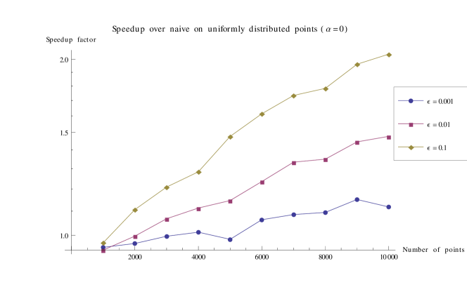
Refer to caption
Figure 10: Speedup result on uniformly distributed points using the deterministic algorithm (α=0𝛼0\alpha=0). The base timings for the naive algorithm on each point set are: 1.91×1011.91superscript1011.91\times 10^{1} seconds, 1.54×1021.54superscript1021.54\times 10^{2} seconds, 5.17×1025.17superscript1025.17\times 10^{2} seconds, 1.23×1031.23superscript1031.23\times 10^{3} seconds, 2.39×1032.39superscript1032.39\times 10^{3} seconds, 4.16×1034.16superscript1034.16\times 10^{3} seconds, 6.64×1036.64superscript1036.64\times 10^{3} seconds, 9.76×1039.76superscript1039.76\times 10^{3} seconds, 1.43×1041.43superscript1041.43\times 10^{4} seconds, and 1.92×1041.92superscript1041.92\times 10^{4} seconds.

6.2 Multibody Computation

We demonstrate speedup results of our approximate algorithms guaranteeing the (1α)1𝛼(1-\alpha) probabilistic ϵitalic-ϵ\epsilon relative error criterion (Definition 2.3). For this paper, we focus strictly on the relative error criterion (τ=0𝜏0\tau=0) and test on three relative error parameter values ( ϵ=0.001italic-ϵ0.001\epsilon=0.001, ϵ=0.01italic-ϵ0.01\epsilon=0.01, and ϵ=0.1italic-ϵ0.1\epsilon=0.1). We test on three different types of distribution: uniform within the unit hypercube [0,1]3superscript013[0,1]^{3} (denoted as the “uniform” distribution), the annulus distribution (denoted as the “annulus” distribution) in three dimensions, and uniform within the unit three-dimensional sphere (denoted as the “ball” distribution). These three distributions were also used in [24]). For the deterministic and probabilistic algorithms, the order of local expansion is fixed at p=0𝑝0p=0 and only 00-th order multipole expansions are used for the results.

Deterministic Approximations. Figure 10, Figure 12, and Figure 11 show speedup results against the naive algorithm using only the deterministic approximation (i.e. α=0𝛼0\alpha=0). On the uniform distribution and the ball distribution, the speedup is almost non-existent; the speedup factor is a little bit more than two on the dataset containing 10,0001000010,000 points using the lowest parameter setting of ϵ=0.1italic-ϵ0.1\epsilon=0.1. On the annulus distribution, our deterministic algorithm achieves a little bit better speedup against the naive algorithm; a factor of more than 20 times speedup on 10,0001000010,000 points is encountered on ϵ=0.1italic-ϵ0.1\epsilon=0.1. A tree-based hierarchical method generally works better for clustered point sets, and this is reflected in our results.
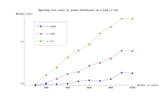
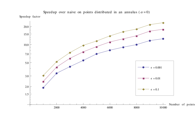
Refer to caption
Figure 11: Speedup result on points distributed inside a sphere using the deterministic algorithm (α=0𝛼0\alpha=0). The base timings for the naive algorithms are listed in Figure 10.
Refer to caption
Figure 12: Speedup result on points distributed on an annulus using the deterministic algorithm (α=0𝛼0\alpha=0). The base timings for the naive algorithms are listed in Figure 10.

Monte-Carlo Approximations. In this section, we show whether adding indeterminism by sampling can reduce the computation time while guaranteeing a slightly relaxed error criterion (but with a high probability guarantee for each potential sum). We first relax the probability guarantee to be 90%percent9090\% (i.e. α=0.1𝛼0.1\alpha=0.1). Like the results shown using the deterministic algorithm, our Monte Carlo-based algorithm achieves the most speedup on points distributed in an annulus (100010001000 times speedup on 10,0001000010,000 points using ϵ=0.1italic-ϵ0.1\epsilon=0.1). See Figure 13, Figure 14, and Figure 15.
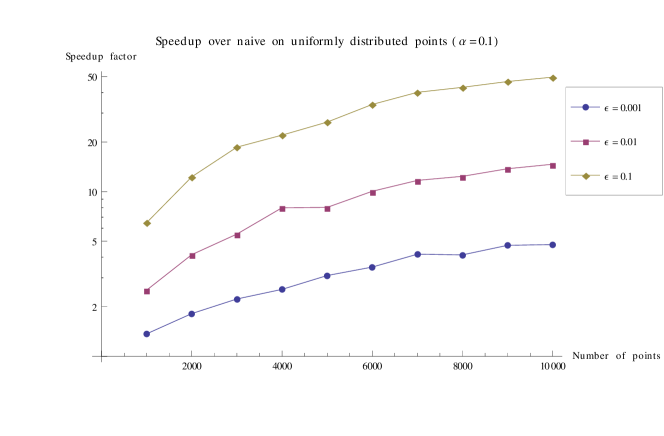
Refer to caption
Figure 13: Speedup result on uniformly distributed points using the Monte Carlo-based algorithm (α=0.1𝛼0.1\alpha=0.1). The base timings for the naive algorithms are listed in Figure 10.
Refer to caption
Figure 14: Speedup result on points distributed inside a sphere using the Monte Carlo-based algorithm (α=0.1𝛼0.1\alpha=0.1). The base timings for the naive algorithms are listed in Figure 10.
Refer to caption
Figure 15: Speedup result on points distributed on an annulus using the Monte Carlo-based algorithm (α=0.1𝛼0.1\alpha=0.1). The base timings for the naive algorithms are listed in Figure 10.

We also list the percentage of the points actually achieving the ϵitalic-ϵ\epsilon relative error bound along with the mean and the variance in Table 1, Table 2, and Table 3. The relative error level of 0.0010.0010.001 and the probability guarantee of 90%percent9090\% was used. Under all three distributions, the percentage of points whose potential sum achieved the desired relative error of 0.0010.0010.001 was well above 90%percent9090\%. We list the average relative error, the variance, and the maximum relative error. Note that the maximum relative error can exceed 100%percent100100\% if the true potential sum and its approximation have opposite signs. For a particle with a small potential sum, we have observed that this is indeed the case due to numerical inaccuracies accumulated during the summation.

Number of points % achieving Average relative error Variance Maximum relative error
1000 98.3%percent98.398.3\% 1.11×1041.11superscript1041.11\times 10^{-4} 8.89×1078.89superscript1078.89\times 10^{-7} 2.86×1022.86superscript1022.86\times 10^{-2}
2000 97.9%percent97.997.9\% 1.28×1041.28superscript1041.28\times 10^{-4} 7.71×1077.71superscript1077.71\times 10^{-7} 2.78×1022.78superscript1022.78\times 10^{-2}
3000 98.6%percent98.698.6\% 1.51×1041.51superscript1041.51\times 10^{-4} 2.64×1062.64superscript1062.64\times 10^{-6} 6.47×1026.47superscript1026.47\times 10^{-2}
4000 98.3%percent98.398.3\% 1.44×1041.44superscript1041.44\times 10^{-4} 3.37×1063.37superscript1063.37\times 10^{-6} 1.01×1011.01superscript1011.01\times 10^{-1}
5000 98.7%percent98.798.7\% 2.65×1042.65superscript1042.65\times 10^{-4} 1.09×1041.09superscript1041.09\times 10^{-4} 7.36×1017.36superscript1017.36\times 10^{-1}
6000 98.3%percent98.398.3\% 1.29×1041.29superscript1041.29\times 10^{-4} 1.39×1061.39superscript1061.39\times 10^{-6} 3.62×1023.62superscript1023.62\times 10^{-2}
7000 98.4%percent98.498.4\% 1.86×1041.86superscript1041.86\times 10^{-4} 9.29×1069.29superscript1069.29\times 10^{-6} 1.96×1011.96superscript1011.96\times 10^{-1}
8000 98.8%percent98.898.8\% 9.89×1059.89superscript1059.89\times 10^{-5} 1.21×1061.21superscript1061.21\times 10^{-6} 6.50×1026.50superscript1026.50\times 10^{-2}
9000 98.8%percent98.898.8\% 9.94×1059.94superscript1059.94\times 10^{-5} 1.39×1061.39superscript1061.39\times 10^{-6} 6.69×1026.69superscript1026.69\times 10^{-2}
10000 98.9%percent98.998.9\% 1.02×1041.02superscript1041.02\times 10^{-4} 1.95×1061.95superscript1061.95\times 10^{-6} 1.06×1011.06superscript1011.06\times 10^{-1}
Table 1: The distribution of relative error on the uniform distribution using α=0.1𝛼0.1\alpha=0.1 and ϵ=0.001italic-ϵ0.001\epsilon=0.001.
Number of points % achieving Average relative error Variance Maximum relative error
1000 98.6%percent98.698.6\% 8.21×1058.21superscript1058.21\times 10^{-5} 1.17×1071.17superscript1071.17\times 10^{-7} 7.22×1037.22superscript1037.22\times 10^{-3}
2000 98.7%percent98.798.7\% 1.35×1041.35superscript1041.35\times 10^{-4} 1.26×1061.26superscript1061.26\times 10^{-6} 2.78×1022.78superscript1022.78\times 10^{-2}
3000 98.7%percent98.798.7\% 1.11×1041.11superscript1041.11\times 10^{-4} 7.58×1077.58superscript1077.58\times 10^{-7} 3.23×1023.23superscript1023.23\times 10^{-2}
4000 97.0%percent97.097.0\% 1.36×1031.36superscript1031.36\times 10^{-3} 1.21×1031.21superscript1031.21\times 10^{-3} 1.81×1001.81superscript1001.81\times 10^{0}
5000 98.2%percent98.298.2\% 1.19×1041.19superscript1041.19\times 10^{-4} 1.18×1061.18superscript1061.18\times 10^{-6} 4.85×1024.85superscript1024.85\times 10^{-2}
6000 98.9%percent98.998.9\% 1.20×1041.20superscript1041.20\times 10^{-4} 3.70×1063.70superscript1063.70\times 10^{-6} 1.27×1011.27superscript1011.27\times 10^{-1}
7000 98.8%percent98.898.8\% 1.22×1041.22superscript1041.22\times 10^{-4} 3.32×1063.32superscript1063.32\times 10^{-6} 1.11×1011.11superscript1011.11\times 10^{-1}
8000 98.5%percent98.598.5\% 1.31×1041.31superscript1041.31\times 10^{-4} 3.67×1063.67superscript1063.67\times 10^{-6} 1.12×1011.12superscript1011.12\times 10^{-1}
9000 97.9%percent97.997.9\% 6.24×1046.24superscript1046.24\times 10^{-4} 3.89×1043.89superscript1043.89\times 10^{-4} 1.14×1001.14superscript1001.14\times 10^{0}
10000 97.6%percent97.697.6\% 5.09×1045.09superscript1045.09\times 10^{-4} 2.40×1042.40superscript1042.40\times 10^{-4} 1.28×1001.28superscript1001.28\times 10^{0}
Table 2: The distribution of relative error on the ball distribution using α=0.1𝛼0.1\alpha=0.1 and ϵ=0.001italic-ϵ0.001\epsilon=0.001.
Number of points % achieving Average relative error Variance Maximum relative error
1000 98.4%percent98.498.4\% 9.33×1059.33superscript1059.33\times 10^{-5} 3.42×1073.42superscript1073.42\times 10^{-7} 1.38×1021.38superscript1021.38\times 10^{-2}
2000 97.2%percent97.297.2\% 9.21×1049.21superscript1049.21\times 10^{-4} 2.69×1042.69superscript1042.69\times 10^{-4} 5.15×1015.15superscript1015.15\times 10^{-1}
3000 98.7%percent98.798.7\% 8.52×1058.52superscript1058.52\times 10^{-5} 1.16×1061.16superscript1061.16\times 10^{-6} 5.09×1025.09superscript1025.09\times 10^{-2}
4000 91.8%percent91.891.8\% 2.53×1022.53superscript1022.53\times 10^{-2} 6.10×1016.10superscript1016.10\times 10^{-1} 4.80×1014.80superscript1014.80\times 10^{1}
5000 96.9%percent96.996.9\% 1.28×1031.28superscript1031.28\times 10^{-3} 1.09×1031.09superscript1031.09\times 10^{-3} 1.27×1001.27superscript1001.27\times 10^{0}
6000 92.8%percent92.892.8\% 6.28×1036.28superscript1036.28\times 10^{-3} 1.38×1021.38superscript1021.38\times 10^{-2} 6.43×1006.43superscript1006.43\times 10^{0}
7000 95.2%percent95.295.2\% 2.13×1032.13superscript1032.13\times 10^{-3} 1.36×1031.36superscript1031.36\times 10^{-3} 6.66×1046.66superscript1046.66\times 10^{-4}
8000 91.2%percent91.291.2\% 1.45×1021.45superscript1021.45\times 10^{-2} 3.77×1013.77superscript1013.77\times 10^{-1} 5.36×1015.36superscript1015.36\times 10^{1}
9000 94.6%percent94.694.6\% 5.17×1035.17superscript1035.17\times 10^{-3} 6.56×1036.56superscript1036.56\times 10^{-3} 3.94×1003.94superscript1003.94\times 10^{0}
10000 91.6%percent91.691.6\% 2.72×1022.72superscript1022.72\times 10^{-2} 8.06×1018.06superscript1018.06\times 10^{-1} 8.29×1018.29superscript1018.29\times 10^{1}
Table 3: The distribution of relative error on the annulus distribution using α=0.1𝛼0.1\alpha=0.1 and ϵ=0.001italic-ϵ0.001\epsilon=0.001.

7 Conclusion

In this paper, we have introduced the framework for extending the pairwise series expansion to potentials that involve more than two points. Through this process, we have formally defined an analogue to the far-field expansion for approximating the multibody potentials in a hierarchical fashion as done in traditional FMM algorithms and have derived algorithms for guaranteeing (1) absolute error bound (2) relative error bound (3) probabilistic absolute/relative error on each particle potential sum and proved the correctness of our algorithms formally. However, we do not present a full-fledged derivation of all three translation operators and the analogue to the local expansion due to a technical difficulty. Instead, we propose to use only a monopole approximation (p=0𝑝0p=0) in a simpler alternative algorithm. Our experiment demonstrates that the algorithm using the hybrid deterministic/probabilistic approximation heuristic achieves speedup under points lying on an annulus of a sphere (i.e. lower-dimensional manifold). For our future work, we are working on parallelization as done in [25, 26].

References

References

  • [1] B. Axilrod, E. Teller, Interaction of the van der Waals type between three atoms, The Journal of Chemical Physics 11 (1943) 299.
  • [2] H. Cheng, L. Greengard, V. Rokhlin, A fast adaptive multipole algorithm in three dimensions, Journal of Computational Physics 155 (2) (1999) 468–498.
  • [3] L. Greengard, J. Huang, A new version of the fast multipole method for screened Coulomb interactions in three dimensions, Journal of Computational Physics 180 (2) (2002) 642–658.
  • [4] L. Greengard, J. Strain, The Fast Gauss Transform, SIAM Journal of Scientific and Statistical Computing 12(1) (1991) 79–94.
  • [5] A. Gray, A. W. Moore, N-Body Problems in Statistical Learning, in: T. K. Leen, T. G. Dietterich, V. Tresp (Eds.), Advances in Neural Information Processing Systems 13 (December 2000), MIT Press, 2001.
  • [6] C. Yang, R. Duraiswami, N. A. Gumerov, L. Davis, Improved fast gauss transform and efficient kernel density estimation, International Conference on Computer Vision.
  • [7] P. Martinsson, V. Rokhlin, Y. U. D. of Computer Science, An accelerated kernel-independent fast multipole method in one dimension, SIAM Journal on Scientific Computing 29 (3) (2008) 1160.
  • [8] S. Kapur, D. Long, IES 3: efficient electrostatic and electromagneticsimulation, IEEE Computational Science & Engineering 5 (4) (1998) 60–67.
  • [9] C. Anderson, An implementation of the fast multipole method without multipoles, SIAM Journal on Scientific and Statistical Computing 13 (1992) 923.
  • [10] L. Ying, G. Biros, D. Zorin, A kernel-independent adaptive fast multipole algorithm in two and three dimensions, Journal of Computational Physics 196 (2) (2004) 591–626.
  • [11] G. Marcelli, The Role of Three-Body Interactions on the Equilibrium and Non-Equilibrium Properties of Fluids from Molecular Simulation, PhD. Thesis, Swinburne University of Technology, Department of Computer Science (2001).
  • [12] G. Marcelli, B. Todd, R. Sadus, Beyond traditional effective intermolecular potentials and pairwise interactions in molecular simulation, Computational Science—ICCS 2002 (2009) 932–941.
  • [13] J. L. Bentley, Multidimensional Binary Search Trees used for Associative Searching, Communications of the ACM 18 (1975) 509–517.
  • [14] A. G. Gray, A. W. Moore, Nonparametric Density Estimation: Toward Computational Tractability, in: SIAM International Conference on Data Mining, 2003.
  • [15] A. Gray, A. Moore, Very fast multivariate kernel density estimation via computational geometry, in: Joint Stat. Meeting, 2003.
  • [16] A. Gray, A. Moore, Rapid evaluation of multiple density models, 2003.
  • [17] A. Moore, A. Connolly, C. Genovese, A. Gray, L. Grone, N. Kanidoris, R. Nichol, J. Schneider, A. Szalay, I. Szapudi, L. Wasserman, Fast algorithms and efficient statistics: N-point correlation functions, in: Proceedings of MPA/MPE/ESO Conference Mining the Sky, July 31–August 4, Garching, Germany, 2000.
  • [18] D. Lee, A. G. Gray, A. W. Moore, Dual-tree fast gauss transforms (2011). arXiv:arXiv:1102.2878.
  • [19] M. Holmes, A. Gray, C. Isbell Jr, Fast kernel conditional density estimation: A dual-tree Monte Carlo approach, Computational Statistics & Data Analysis 54 (7) (2010) 1707–1718.
  • [20] M. Holmes, A. Gray, C. Isbell Jr, Ultrafast Monte Carlo for kernel estimators and generalized statistical summations, Advances in Neural Information Processing Systems (NIPS) 21.
  • [21] D. Lee, A. Gray, Fast high-dimensional kernel summations using the monte carlo multipole method, in: In Advances in Neural Information Processing Systems 21, 2009.
  • [22] G. Boyer, R. Riegel, N. Vasiloglou, D. Lee, L. Poorman, C. Mappus, N. Mehta, H. Ouyang, P. Ram, L. Tran, W. C. Wong, A. Gray, MLPACK, http://mloss.org/software/view/152 (2009).
  • [23] R. Curtin, J. Cline, N. Slagle, M. Amidon, A. Kale, B. March, N. Mehta, P. Ram, D. Lee, A. Gray, libmlpack, http://mloss.org/software/view/364/ (2011).
  • [24] J. Bentley, K-d trees for semidynamic point sets, in: Proceedings of the sixth annual symposium on Computational geometry, ACM, 1990, pp. 187–197.
  • [25] J. Li, Z. Zhou, R. Sadus, Modified force decomposition algorithms for calculating three-body interactions via molecular dynamics, Computer Physics Communications 175 (11-12) (2006) 683–691.
  • [26] R. Sampath, H. Sundar, S. Veerapaneni, Parallel Fast Gauss Transform, in: Supercomputing, 2010.