Fast First-Order Methods for Stable Principal Component Pursuit

Abstract

The stable principal component pursuit (SPCP) problem is a non-smooth convex optimization problem, the solution of which has been shown both in theory and in practice to enable one to recover the low rank and sparse components of a matrix whose elements have been corrupted by Gaussian noise. In this paper, we first show how several existing fast first-order methods can be applied to this problem very efficiently. Specifically, we show that the subproblems that arise when applying optimal gradient methods of Nesterov, alternating linearization methods and alternating direction augmented Lagrangian methods to the SPCP problem either have closed-form solutions or have solutions that can be obtained with very modest effort. Later, we develop a new first order algorithm, NSA, based on partial variable splitting. All but one of the methods analyzed require at least one of the non-smooth terms in the objective function to be smoothed and obtain an $\epsilon$-optimal solution to the SPCP problem in $O(1/\epsilon)$ iterations. NSA, which works directly with the fully non-smooth objective function, is proved to be convergent under mild conditions on the sequence of parameters it uses. Our preliminary computational tests show that the latter method, NSA, although its complexity is not known, is the fastest among the four algorithms described and substantially outperforms ASALM, the only existing method for the SPCP problem. To best of our knowledge, an algorithm for the SPCP problem that has $\mathcal{O}(1/\epsilon)$ iteration complexity and has a per iteration complexity equal to that of a singular value decomposition is given for the first time.

1 Introduction

In [2, 12], it was shown that when the data matrix $D\in\mathbb{R}^{m\times n}$ is of the form $D=X^{0}+S^{0}$, where $X^{0}$ is a low-rank matrix, i.e. $\mathop{\bf rank}(X^{0})\ll\min\{m,n\}$, and $S^{0}$ is a sparse matrix, i.e. $\|S^{0}\|_{0}\ll mn$ ($\|.\|_{0}$ counts the number of nonzero elements of its argument), one can recover the low-rank and sparse components of $D$ by solving the principal component pursuit problem

$$\min_{X\in\mathbb{R}^{m\times n}}\|X\|_{*}+\xi~{}\|D-X\|_{1},$$ (1)

where $\xi=\frac{1}{\sqrt{\max\{m,n\}}}$.

For $X\in\mathbb{R}^{m\times n}$, $\|X\|_{*}$ denotes the nuclear norm of $X$, which is equal to the sum of its singular values, $\|X\|_{1}:=\sum_{i=1}^{m}\sum_{j=1}^{n}|X_{ij}|$, $\|X\|_{\infty}:=\max\{|X_{ij}|:~{}1\leq i\leq m,~{}1\leq j\leq n\}$ and $\|X\|_{2}:=\sigma_{\rm max}(X)$, where $\sigma_{\rm max}(X)$ is the maximum singular value of $X$.

To be more precise, let $X^{0}\in\mathbb{R}^{m\times n}$ with $\mathop{\bf rank}(X^{0})=r$ and let $X^{0}=U\Sigma V^{T}=\sum_{i=1}^{r}\sigma_{i}u_{i}v_{i}^{T}$ denote the singular value decomposition (SVD) of $X^{0}$. Suppose that for some $\mu>0$, $U$ and $V$ satisfy

$$\max_{i}\|U^{T}e_{i}\|_{2}^{2}\leq\frac{\mu r}{m},\quad\max_{i}\|V^{T}e_{i}\|_{2}^{2}\leq\frac{\mu r}{n},\quad\|UV^{T}\|_{\infty}\leq\sqrt{\frac{\mu r}{mn}},$$ (2)

where $e_{i}$ denotes the $i$-th unit vector.

Theorem 1.

[2] Suppose $D=X^{0}+S^{0}$, where $X^{0}\in\mathbb{R}^{m\times n}$ with $m<n$ satisfies (2) for some $\mu>0$, and the support set of $S^{0}$ is uniformly distributed. Then there are constants $c$, $\rho_{r}$, $\rho_{s}$ such that with probability of at least $1-cn^{-10}$, the principal component pursuit problem (1) exactly recovers $X^{0}$ and $S^{0}$ provided that

$$\mathop{\bf rank}(X^{0})\leq\rho_{r}m\mu^{-1}(\log(n))^{-2}\quad\mbox{and}\quad\|S^{0}\|_{0}\leq\rho_{s}mn.$$ (3)

In [13], it is shown that the recovery is still possible even when the data matrix, $D$, is corrupted with a dense error matrix, $\zeta^{0}$ such that $\|\zeta^{0}\|_{F}\leq\delta$, by solving the stable principal component pursuit (SPCP) problem

$$(P):\min_{X,S\in\mathbb{R}^{m\times n}}\{\|X\|_{*}+\xi~{}\|S\|_{1}:\ \|X+S-D\|_{F}\leq\delta\}.$$ (4)

Specifically, the following theorem is proved in [13].

Theorem 2.

[13] Suppose $D=X^{0}+S^{0}+\zeta^{0}$, where $X^{0}\in\mathbb{R}^{m\times n}$ with $m<n$ satisfies (2) for some $\mu>0$, and the support set of $S^{0}$ is uniformly distributed. If $X^{0}$ and $S^{0}$ satisfy (3), then for any $\zeta^{0}$ such that $\|\zeta^{0}\|_{F}\leq\delta$ the solution, $(X^{*},S^{*})$, to the stable principal component pursuit problem (4) satisfies $\|X^{*}-X^{0}\|_{F}^{2}+\|S^{*}-S^{0}\|_{F}^{2}\leq Cmn\delta^{2}$ for some constant $C$ with high probability.

Principal component pursuit and stable principal component pursuit both have applications in video surveillance and face recognition. For existing algorithmic approaches to solving principal component pursuit see  [2, 3, 6, 7, 13] and references therein. In this paper, we develop four different fast first-order algorithms to solve the SPCP problem $(P)$. The first two algorithms are direct applications of Nesterov’s optimal algorithm [9] and the proximal gradient method of Tseng [11], which is inspired by both FISTA and Nesterov’s infinite memory algorithms that are introduced in [1] and [9], respectively. In this paper it is shown that both algorithms can compute an $\epsilon$-optimal, feasible solution to $(P)$ in $\mathcal{O}(1/\epsilon)$ iterations. The third and fourth algorithms apply an alternating direction augmented Lagrangian approach to an equivalent problem obtained by partial variable splitting. The third algorithm can compute an $\epsilon$-optimal, feasible solution to the problem in $\mathcal{O}(1/\epsilon^{2})$ iterations, which can be easily improved to $\mathcal{O}(1/\epsilon)$ complexity. Given $\epsilon>0$, all first three algorithms use suitably smooth versions of at least one of the norms in the objective function. The fourth algorithm (NSA) works directly with the original non-smooth objective function and can be shown to converge to an optimal solution of $(P)$, provided that a mild condition on the increasing sequence of penalty multipliers holds. To best of our knowledge, an algorithm for the SPCP problem that has $\mathcal{O}(1/\epsilon)$ iteration complexity and has a per iteration complexity equal to that of a singular value decomposition is given for the first time.

The only algorithm that we know of that has been designed to solve the SPCP problem $(P)$ is the algorithm ASALM [10]. The results of our numerical experiments comparing NSA algorithm with ASALM has shown that NSA is faster and also more robust to changes in problem parameters.

2 Proximal Gradient Algorithm with Smooth Objective Function

In this section we show that Nesterov’s optimal algorithm [8, 9] for simple sets is efficient for solving $(P)$.

For fixed parameters $\mu>0$ and $\nu>0$, define the smooth $C^{1,1}$ functions $f_{\mu}(.)$ and $g_{\nu}(.)$ as follows

$$f_{\mu}(X)=\max_{U\in\mathbb{R}^{m\times n}:\|U\|_{2}\leq 1}\langle X,U\rangle-\frac{\mu}{2}\|U\|_{F}^{2},$$ (5)

$$g_{\nu}(S)=\max_{W\in\mathbb{R}^{m\times n}:\|W\|_{\infty}\leq 1}\langle S,W\rangle-\frac{\nu}{2}\|W\|_{F}^{2}.$$ (6)

Clearly, $f_{\mu}(.)$ and $g_{\nu}(.)$ closely approximate the non-smooth functions $f(X):=\|X\|_{*}$ and $g(S):=\|S\|_{1}$, respectively. Also let $\chi:=\{(X,S)\in\mathbb{R}^{m\times n}\times\mathbb{R}^{m\times n}:~{}\|X+S-D\|_{F}\leq\delta\}$ and $L=\frac{1}{\mu}+\frac{1}{\nu}$, where $\frac{1}{\mu}$ and $\frac{1}{\nu}$ are the Lipschitz constants for the gradients of $f_{\mu}(.)$ and $g_{\nu}(.)$, respectively. Then Nesterov’s optimal algorithm [8, 9] for simple sets applied to the problem:

$$\min_{X,S\in\mathbb{R}^{m\times n}}\{f_{\mu}(X)+\xi~{}g_{\nu}(S):\ (X,S)\in\chi\},$$ (7)

is given by Algorithm 1.

Algorithm 1 SMOOTH PROXIMAL GRADIENT($X_{0},S_{0}$)

1:  input: $X_{0}\in\mathbb{R}^{m\times n}$, $S_{0}\in\mathbb{R}^{m\times n}$

2:  $k\leftarrow 0$

3:  while $k\leq k^{*}$ do

4:     Compute $\nabla f_{\mu}(X_{k})$ and $\nabla g_{\nu}(S_{k})$

5:     $(Y^{x}_{k},Y^{s}_{k})\leftarrow\mathop{\rm argmin}_{X,S}\left\{\langle\nabla f_{\mu}(X_{k}),X\rangle+\langle\nabla g_{\nu}(S_{k}),S\rangle+\frac{L}{2}\left(\|X-X_{k}\|_{F}^{2}+\|S-S_{k}\|_{F}^{2}\right):\ (X,S)\in\chi\right\}$

6:     $\Gamma_{k}(X,S):=\sum_{i=0}^{k}\frac{i+1}{2}\left\{\langle\nabla f_{\mu}(X_{i}),X\rangle+\langle\nabla g_{\nu}(S_{i}),S\rangle\right\}$

7:     $(Z^{x}_{k},Z^{s}_{k})\leftarrow\mathop{\rm argmin}_{X,S}\left\{\Gamma_{k}(X,S)+\frac{L}{2}\left(\|X-X_{0}\|_{F}^{2}+\|S-S_{0}\|_{F}^{2}\right):(X,S)\in\chi\right\}$

8:     $(X_{k+1},S_{k+1})\leftarrow\left(\frac{k+1}{k+3}\right)(Y^{x}_{k},Y^{s}_{k})+\left(\frac{2}{k+3}\right)(Z^{x}_{k},Z^{s}_{k})$

9:     $k\leftarrow k+1$

10:  end while

11:  return  $(X_{k^{*}},S_{k^{*}})$

Because of the simple form of the set $\chi$, it is easy to ensure that all iterates $(Y^{x}_{k},Y^{s}_{k})$, $(Z^{x}_{k},Z^{s}_{k})$ and $(X_{k+1},S_{k+1})$ lie in $\chi$. Hence, Algorithm 1 enjoys the full convergence rate of $\mathcal{O}(L/k^{2})$ of the Nesterov’s method. Thus, setting $\mu=\Omega(\epsilon)$ and $\nu=\Omega(\epsilon)$, Algorithm 1 computes an $\epsilon$-optimal and feasible solution to problem $(P)$ in $k^{*}=\mathcal{O}(1/\epsilon)$ iterations. The iterates $(Y^{x}_{k},Y^{s}_{k})$ and $(Z^{x}_{k},Z^{s}_{k})$ that need to be computed at each iteration of Algorithm 1 are solutions to an optimization problem of the form:

$$(P_{s}):\ \min_{X,S\in\mathbb{R}^{m\times n}}\left\{\frac{L}{2}\left(\|X-\tilde{X}\|_{F}^{2}+\|S-\tilde{S}\|_{F}^{2}\right)+\langle Q_{x},X\rangle+\langle Q_{s},S\rangle:\ (X,S)\in\chi\right\}.$$ (8)

The following lemma shows that the solution to problems of the form $(P_{s})$ can be computed efficiently.

Lemma 3.

The optimal solution $(X^{*},S^{*})$ to problem $(P_{s})$ can be written in closed form as follows.

When $\delta>0$,

$$X^{*}=\left(\frac{\theta^{*}}{L+2\theta^{*}}\right)\left(D-q_{s}(\tilde{S})\right)+\left(\frac{L+\theta^{*}}{L+2\theta^{*}}\right)q_{x}(\tilde{X}),$$ (9)

$$S^{*}=\left(\frac{\theta^{*}}{L+2\theta^{*}}\right)\left(D-q_{x}(\tilde{X})\right)+\left(\frac{L+\theta^{*}}{L+2\theta^{*}}\right)q_{s}(\tilde{S}),$$ (10)

where $q_{x}(X):=X-\frac{1}{L}~{}Q_{x}$, $q_{s}(S):=S-\frac{1}{L}~{}Q_{s}$ and

$$\theta^{*}=\max\left\{0,~{}\frac{L}{2}\left(\frac{\|q_{x}(\tilde{X})+q_{s}(\tilde{S})-D\|_{F}}{\delta}-1\right)\right\}.$$ (11)

When $\delta=0$,

$$\begin{array}[]{ll}X^{*}=\frac{1}{2}\left(D-q_{s}(\tilde{S})\right)+\frac{1}{2}~{}q_{x}(\tilde{X})\hbox{ and}&S^{*}=\frac{1}{2}\left(D-q_{x}(\tilde{X})\right)+\frac{1}{2}~{}q_{s}(\tilde{S}).\end{array}$$ (12)

Proof.

Suppose that $\delta>0$. Writing the constraint in problem $(P_{s})$, $(X,S)\in\chi$, as

$$\frac{1}{2}\|X+S-D\|^{2}_{F}\leq\frac{\delta^{2}}{2},$$ (13)

the Lagrangian function for (8) is given as

$$\mathcal{L}(X,S;\theta)=\frac{L}{2}\left(\|X-\tilde{X}\|_{F}^{2}+\|S-\tilde{S}\|_{F}^{2}\right)+\langle Q_{x},X-\tilde{X}\rangle+\langle Q_{s},S-\tilde{S}\rangle+\frac{\theta}{2}\left(\|X+S-D\|_{F}^{2}-\delta^{2}\right).$$

Therefore, the optimal solution $(X^{*},S^{*})$ and optimal Lagrangian multiplier $\theta^{*}\in\mathbb{R}$ must satisfy the Karush-Kuhn-Tucker (KKT) conditions:

1. $\|X^{*}+S^{*}-D\|_{F}\leq\delta$,

2. $\theta^{*}\geq 0$,

3. $\theta^{*}~{}(\|X^{*}+S^{*}-D\|_{F}-\delta)=0$,

4. $L(X^{*}-\tilde{X})+\theta^{*}(X^{*}+S^{*}-D)+Q_{x}=0$,

5. $L(S^{*}-\tilde{S})+\theta^{*}(X^{*}+S^{*}-D)+Q_{s}=0$.

Conditions iv and v imply that $(X^{*},S^{*})$ satisfy $\eqref{lemeq:X_smooth}$ and (10), from which it follows that

$$X^{*}+S^{*}-D=\left(\frac{L}{L+2\theta^{*}}\right)\left(q_{x}(\tilde{X})+q_{s}(\tilde{S})-D\right).$$ (14)

Case 1: $\|q_{x}(\tilde{X})+q_{s}(\tilde{S})-D\|_{F}\leq\delta$

Setting $X^{*}=q_{x}(\tilde{X})$, $S^{*}=q_{s}(\tilde{S})$ and $\theta^{*}=0$, clearly satisfies $\eqref{lemeq:X_smooth}$, (10) and conditions i (from (14)), ii and iii. Thus, this choice of variables satisfies all the five KKT conditions.

Case 2: $\|q_{x}(\tilde{X})+q_{s}(\tilde{S})-D\|_{F}>\delta$

Set $\theta^{*}=\frac{L}{2}\left(\frac{\|q_{x}(\tilde{X})+q_{s}(\tilde{S})-D\|_{F}}{\delta}-1\right)$. Since $\|q_{x}(\tilde{X})+q_{s}(\tilde{S})-D\|_{F}>\delta$, $\theta^{*}>0$; hence, ii is satisfied. Moreover, for this value of $\theta^{*}$, it follows from (14) that $\|X^{*}+S^{*}-D\|_{F}=\delta$. Thus, KKT conditions i and iii are satisfied.

Therefore, setting $X^{*}$ and $S^{*}$ according to (9) and (10), respectively; and setting

$$\theta^{*}=\max\left\{0,\ \frac{L}{2}\left(\frac{\|q_{x}(\tilde{X})+q_{s}(\tilde{S})-D\|_{F}}{\delta}-1\right)\right\},$$

satisfies all the five KKT conditions.

Now, suppose that $\delta=0$. Since $S^{*}=D-X^{*}$, problem $(P_{s})$can be written as

$$\begin{array}[]{ll}\min_{X\in\mathbb{R}^{m\times n}}&\|X-\tilde{X}+\frac{Q_{x}}{L}\|_{F}^{2}+\|D-X-\tilde{S}+\frac{Q_{s}}{L}\|_{F}^{2},\end{array}$$

which is also equivalent to the problem: $\min_{X\in\mathbb{R}^{m\times n}}\|X-q_{x}(\tilde{X})\|_{F}^{2}+\|X-(D-q_{s}(\tilde{S}))\|_{F}^{2}$. Then (12) trivially follows from first-order optimality conditions for this problem and the fact that $S^{*}=D-X^{*}$. ∎

3 Proximal Gradient Algorithm with Partially Smooth Objective Function

In this section we show how the proximal gradient algorithm, Algorithm 3 in [11], can be applied to the problem

$$\min_{X,S\in\mathbb{R}^{m\times n}}\{f_{\mu}(X)+\xi~{}\|S\|_{1}:\ (X,S)\in\chi\},$$ (15)

where $f_{\mu}(.)$ is the smooth function defined in (5) such that $\nabla f_{\mu}(.)$ is Lipschitz continuous with constant $L_{\mu}=\frac{1}{\mu}$. This algorithm is given in Algorithm 2.

Algorithm 2 PARTIALLY SMOOTH PROXIMAL GRADIENT($X_{0},S_{0}$)

1:  input: $X_{0}\in\mathbb{R}^{m\times n}$, $S_{0}\in\mathbb{R}^{m\times n}$

2:  $(Z^{x}_{0},Z^{s}_{0})\leftarrow(X_{0},S_{0})$, $k\leftarrow 0$

3:  while $k\leq k^{*}$ do

4:     $(Y^{x}_{k},Y^{s}_{k})\leftarrow\left(\frac{k}{k+2}\right)(X_{k},S_{k})+\left(\frac{2}{k+2}\right)(Z^{x}_{k},Z^{s}_{k})$

5:     Compute $\nabla f_{\mu}(Y^{x}_{k})$

6:     $(Z^{x}_{k+1},Z^{s}_{k+1})\leftarrow\mathop{\rm argmin}_{X,S}\left\{\sum_{i=0}^{k}\frac{i+1}{2}\left\{\xi\|S\|_{1}+\langle\nabla f_{\mu}(Y^{x}_{i}),X\rangle\right\}+\frac{L_{\mu}}{2}\|X-X_{0}\|_{F}^{2}:\ (X,S)\in\chi\right\}$

7:     $(X_{k+1},S_{k+1})\leftarrow\left(\frac{k}{k+2}\right)(X_{k},S_{k})+\left(\frac{2}{k+2}\right)(Z^{x}_{k+1},Z^{s}_{k+1})$

8:     $k\leftarrow k+1$

9:  end while

10:  return  $(X_{k^{*}},S_{k^{*}})$

Mimicking the proof in [11], it is easy to show that Algorithm 2, which uses the prox function $\frac{1}{2}\|X-X_{0}\|_{F}^{2}$, converges to the optimal solution of (15). Given $(X_{0},S_{0})\in\chi$, e.g. $X_{0}=\mathbf{0}$ and $S_{0}=D$, the current algorithm keeps all iterates in $\chi$ as in Algorithm 1, and hence it enjoys the full convergence rate of $\mathcal{O}(L/k^{2})$. Thus, setting $\mu=\Omega(\epsilon)$, Algorithm 2 computes an $\epsilon$-optimal, feasible solution of problem $(P)$ in $k^{*}=\mathcal{O}(1/\epsilon)$ iterations.

The only thing left to be shown is that the optimization subproblems in Algorithm 2 can be solved efficiently. The subproblem that has to be solved at each iteration to compute $(Z^{x}_{k+1},Z^{s}_{k+1})$ has the form:

$$(P_{ns}):\ \min\left\{\xi\|S\|_{1}+\langle Q,X-\tilde{X}\rangle+\frac{\rho}{2}\|X-\tilde{X}\|_{F}^{2}:\ (X,S)\in\chi\right\},$$ (16)

for some $\rho>0$. Lemma 4 shows that these computations can be done efficiently.

Lemma 4.

The optimal solution $(X^{*},S^{*})$ to problem $(P_{ns})$ can be written in closed form as follows.

When $\delta>0$,

$$S^{*}=sign\left(D-q(\tilde{X})\right)\odot\max\left\{|D-q(\tilde{X})|-\xi\frac{(\rho+\theta^{*})}{\rho\theta^{*}}~{}E,\ \mathbf{0}\right\},$$ (17)

$$X^{*}=\frac{\theta^{*}}{\rho+\theta^{*}}~{}(D-S^{*})+\frac{\rho}{\rho+\theta^{*}}~{}q(\tilde{X}),$$ (18)

where $q(\tilde{X}):=\tilde{X}-\frac{1}{\rho}~{}Q$, $E$ and $\mathbf{0}\in\mathbb{R}^{m\times n}$ are matrices with all components equal to ones and zeros, respectively, and $\odot$ denotes the componentwise multiplication operator. $\theta^{*}=0$ if $\|D-q(\tilde{X})\|_{F}\leq\delta$; otherwise, $\theta^{*}$ is the unique positive solution of the nonlinear equation $\phi(\theta)=\delta$, where

$$\phi(\theta):=\|\min\left\{\frac{\xi}{\theta}~{}E,\ \frac{\rho}{\rho+\theta}~{}|D-q(\tilde{X})|\right\}\|_{F}.$$ (19)

Moreover, $\theta^{*}$ can be efficiently computed in $\mathcal{O}(mn\log(mn))$ time.

When $\delta=0$,

$$\begin{array}[]{cc}S^{*}=sign\left(D-q(\tilde{X})\right)\odot\max\left\{|D-q(\tilde{X})|-\frac{\xi}{\rho}~{}E,\ \mathbf{0}\right\}\hbox{ and }&X^{*}=D-S^{*}.\end{array}$$ (20)

Proof.

Suppose that $\delta>0$. Let $(X^{*},S^{*})$ be an optimal solution to problem $(P_{ns})$ and $\theta^{*}$ denote the optimal Lagrangian multiplier for the constraint $(X,S)\in\chi$ written as (13). Then the KKT optimality conditions for this problem are

1. $Q+\rho(X^{*}-\tilde{X})+\theta^{*}(X^{*}+S^{*}-D)=0$,

2. $\xi G+\theta^{*}(X^{*}+S^{*}-D)=0$ and $G\in\partial\|S^{*}\|_{1}$,

3. $\|X^{*}+S^{*}-D\|_{F}\leq\delta$,

4. $\theta^{*}\geq 0$,

5. $\theta^{*}~{}(\|X^{*}+S^{*}-D\|_{F}-\delta)=0$.

From i and ii, we have

$$\left[\begin{array}[]{cc}(\rho+\theta^{*})I&\theta^{*}I\\ \theta^{*}I&\theta^{*}I\\ \end{array}\right]\left[\begin{array}[]{c}X^{*}\\ S^{*}\\ \end{array}\right]=\left[\begin{array}[]{c}\theta^{*}D+\rho~{}q(\tilde{X})\\ \theta^{*}D-\xi G\\ \end{array}\right],$$ (27)

where $q(\tilde{X})=\tilde{X}-\frac{1}{\rho}~{}Q$. From (27) it follows that

$$\left[\begin{array}[]{cc}(\rho+\theta^{*})I&\theta^{*}I\\ 0&\left(\frac{\rho\theta^{*}}{\rho+\theta^{*}}\right)~{}I\\ \end{array}\right]\left[\begin{array}[]{c}X^{*}\\ S^{*}\\ \end{array}\right]=\left[\begin{array}[]{c}\theta^{*}D+\rho~{}q(\tilde{X})\\ \frac{\rho\theta^{*}}{\rho+\theta^{*}}~{}(D-q(\tilde{X}))-\xi G\\ \end{array}\right].$$ (34)

From the second equation in (34), we have

$$\xi\frac{(\rho+\theta^{*})}{\rho\theta^{*}}~{}G+S^{*}+q(\tilde{X})-D=0.$$ (35)

But (35) is precisely the first-order optimality conditions for the “shrinkage” problem

$$\min_{S\in\mathbb{R}^{m\times n}}\left\{\xi\frac{(\rho+\theta^{*})}{\rho\theta^{*}}\|S\|_{1}+\frac{1}{2}\|S+q(\tilde{X})-D\|_{F}^{2}\right\}.$$

Thus, $S^{*}$ is the optimal solution to the “shrinkage” problem and is given by (17). (18) follows from the first equation in (34), and it implies

$$X^{*}+S^{*}-D=\frac{\rho}{\rho+\theta^{*}}~{}(S^{*}+q(\tilde{X})-D).$$ (36)

Therefore,

$$\|X^{*}+S^{*}-D\|_{F} =\frac{\rho}{\rho+\theta^{*}}~{}\|S^{*}+q(\tilde{X})-D\|_{F},$$

$$=\frac{\rho}{\rho+\theta^{*}}~{}\|sign\left(D-q(\tilde{X})\right)\odot\max\left\{|D-q(\tilde{X})|-\xi\frac{(\rho+\theta^{*})}{\rho\theta^{*}}~{}E,\ \mathbf{0}\right\}-\left(D-q(\tilde{X})\right)\|_{F},$$

$$=\frac{\rho}{\rho+\theta^{*}}~{}\|\max\left\{|D-q(\tilde{X})|-\xi\frac{(\rho+\theta^{*})}{\rho\theta^{*}}~{}E,\ \mathbf{0}\right\}-|D-q(\tilde{X})|~{}\|_{F},$$

$$=\frac{\rho}{\rho+\theta^{*}}~{}\|\min\left\{\xi\frac{(\rho+\theta^{*})}{\rho\theta^{*}}~{}E,\ |D-q(\tilde{X})|\right\}\|_{F},$$

$$=\|\min\left\{\frac{\xi}{\theta^{*}}~{}E,\ \frac{\rho}{\rho+\theta^{*}}~{}|D-q(\tilde{X})|\right\}\|_{F},$$ (37)

where the second equation uses (17). Now let $\phi:\mathbb{R}_{+}\rightarrow\mathbb{R}_{+}$ be

$$\phi(\theta):=\|\min\left\{\frac{\xi}{\theta}~{}E,\ \frac{\rho}{\rho+\theta}~{}|D-q(\tilde{X})|\right\}\|_{F}.$$ (38)

Case 1: $\|D-q(\tilde{X})\|_{F}\leq\delta$

$\theta^{*}=0$, $S^{*}=\mathbf{0}$ and $X^{*}=q(\tilde{X})$ trivially satisfy all the KKT conditions.

Case 2: $\|D-q(\tilde{X})\|_{F}>\delta$

It is easy to show that $\phi(.)$ is a strictly decreasing function of $\theta$. Since $\phi(0)=\|D-q(\tilde{X})\|_{F}>\delta$ and $\lim_{\theta\rightarrow\infty}\phi(\theta)=0$, there exists a unique $\theta^{*}>0$ such that $\phi(\theta^{*})=\delta$. Given $\theta^{*}$, $S^{*}$ and $X^{*}$ can then be computed from equations (17) and (18), respectively. Moreover, since $\theta^{*}>0$ and $\phi(\theta^{*})=\delta$, (37) implies that $X^{*}$, $S^{*}$ and $\theta^{*}$ satisfy the KKT conditions.

We now show that $\theta^{*}$ can be computed in $\mathcal{O}(mn\log(mn))$ time. Let $A:=|D-q(\tilde{X})|$ and $0\leq a_{(1)}\leq a_{(2)}\leq...\leq a_{(mn)}$ be the $mn$ elements of the matrix $A$ sorted in increasing order, which can be done in $\mathcal{O}(mn\log(mn))$ time. Defining $a_{(0)}:=0$ and $a_{(mn+1)}:=\infty$, we then have for all $j\in\{0,1,...,mn\}$ that

$$\frac{\rho}{\rho+\theta}~{}a_{(j)}\leq\frac{\xi}{\theta}\leq\frac{\rho}{\rho+\theta}~{}a_{(j+1)}\Leftrightarrow\frac{1}{\xi}~{}a_{(j)}-\frac{1}{\rho}\leq\frac{1}{\theta}\leq\frac{1}{\xi}~{}a_{(j+1)}-\frac{1}{\rho}.$$ (39)

For all $\bar{k}<j\leq mn$ define $\theta_{j}$ such that $\frac{1}{\theta_{j}}=\frac{1}{\xi}~{}a_{(j)}-\frac{1}{\rho}$ and let $\bar{k}:=\max\left\{j:\frac{1}{\theta_{j}}\leq 0,\ j\in\{0,1,...,mn\}\right\}$. Then for all $\bar{k}<j\leq mn$

$$\phi(\theta_{j})=\sqrt{\left(\frac{\rho}{\rho+\theta_{j}}\right)^{2}~{}\sum_{i=0}^{j}a^{2}_{(i)}+(mn-j)~{}\left(\frac{\xi}{\theta_{j}}\right)^{2}}.$$ (40)

Also define $\theta_{\bar{k}}:=\infty$ and $\theta_{mn+1}:=0$ so that $\phi(\theta_{\bar{k}}):=0$ and $\phi(\theta_{mn+1})=\phi(0)=\|A\|_{F}>\delta$. Note that $\{\theta_{j}\}_{\{\bar{k}<j\leq mn\}}$ contains all the points at which $\phi(\theta)$ may not be differentiable for $\theta\geq 0$. Define $j^{*}:=\max\{j:\ \phi(\theta_{j})\leq\delta,\ \bar{k}\leq j\leq mn\}$. Then $\theta^{*}$ is the unique solution of the system

$$\sqrt{\left(\frac{\rho}{\rho+\theta}\right)^{2}~{}\sum_{i=0}^{j^{*}}a^{2}_{(i)}+(mn-j^{*})~{}\left(\frac{\xi}{\theta}\right)^{2}}=\delta\mbox{ and }\theta>0,$$ (41)

since $\phi(\theta)$ is continuous and strictly decreasing in $\theta$ for $\theta\geq 0$. Solving the equation in (41) requires finding the roots of a fourth-order polynomial (a.k.a. quartic function); therefore, one can compute $\theta^{*}>0$ using the algebraic solutions of quartic equations (as shown by Lodovico Ferrari in 1540), which requires $\mathcal{O}(1)$ operations.

Note that if $\bar{k}=mn$, then $\theta^{*}$ is the solution of the equation

$$\sqrt{\left(\frac{\rho}{\rho+\theta^{*}}\right)^{2}~{}\sum_{i=1}^{mn}a^{2}_{(i)}}=\delta,$$ (42)

i.e. $\theta^{*}=\rho\left(\frac{\|A\|_{F}}{\delta}-1\right)=\rho\left(\frac{\|D-\tilde{X}\|_{F}}{\delta}-1\right)$. Hence, we have proved that problem $(P_{ns})$ can be solved efficiently.

Now, suppose that $\delta=0$. Since $S^{*}=D-X^{*}$, problem $(P_{ns})$ can be written as

$$\begin{array}[]{ll}\min_{S\in\mathbb{R}^{m\times n}}&\frac{\xi}{\rho}\|S\|_{1}+\frac{1}{2}\|S-(D-q(\tilde{X}))\|_{F}^{2}.\end{array}$$ (43)

Then (20) trivially follows from first-order optimality conditions for the above problem and the fact that $X^{*}=D-S^{*}$. ∎

The following lemma will be used later in Section 5. However, we give its proof here, since it uses some equations from the proof of Lemma 4. Let $\mathbf{1}_{\chi}(.,.)$ denote the indicator function of the closed convex set $\chi\subset\mathbb{R}^{m\times n}\times\mathbb{R}^{m\times n}$, i.e. if $(Z,S)\in\chi$, then $\mathbf{1}_{\chi}(Z,S)=0$; otherwise, $\mathbf{1}_{\chi}(Z,S)=\infty$.

Lemma 5.

Suppose that $\delta>0$. Let $(X^{*},S^{*})$ be an optimal solution to problem $(P_{ns})$ and $\theta^{*}$ be an optimal Lagrangian multiplier such that $(X^{*},S^{*})$ and $\theta^{*}$ together satisfy the KKT conditions, i-v in the proof of Lemma 4. Then $(W^{*},W^{*})\in\partial\mathbf{1}_{\chi}(X^{*},S^{*})$, where $W^{*}:=-Q+\rho(\tilde{X}-X^{*})=\theta^{*}(X^{*}+S^{*}-D)$.

Proof.

Let $W^{*}:=-Q+\rho(\tilde{X}-X^{*})$, then from i and v of the KKT optimality conditions in the proof of Lemma 4, we have $W^{*}=\theta^{*}(X^{*}+S^{*}-D)$ and

$$\|W^{*}\|_{F}=\theta^{*}\|X^{*}+S^{*}-D\|=\theta^{*}(\|X^{*}+S^{*}-D\|-\delta)+\theta^{*}\delta=\theta^{*}\delta.$$ (44)

Moreover, for all $(X,S)\in\chi$, it follows from the definition of $\chi$ that $\langle W^{*},\theta^{*}(X+S-D)\rangle\leq\theta^{*}\|W^{*}\|_{F}\|X+S-D\|_{F}\leq\theta^{*}\delta\|W^{*}\|_{F}$. Thus, for all $(X,S)\in\chi$, we have $\langle W^{*},W^{*}\rangle=\|W^{*}\|_{F}^{2}=\theta^{*}\delta\|W^{*}\|_{F}\geq\langle W^{*},\theta^{*}(X+S-D)\rangle$. Hence,

$$0\geq\langle W^{*},\theta^{*}(X+S-D)-W^{*}\rangle=\langle W^{*},\theta^{*}(X-X^{*}+S-S^{*})\rangle\hskip 14.22636pt\forall~{}(X,S)\in\chi.$$ (45)

It follows from the proof of Lemma 4 that if $\|D-q(\tilde{X})\|_{F}>\delta$, then $\theta^{*}>0$, where $q(\tilde{X})=\tilde{X}-\frac{1}{\rho}Q$. Therefore, (45) implies that

$$0\geq\langle W^{*},X-X^{*}+S-S^{*}\rangle\hskip 14.22636pt\forall~{}(X,S)\in\chi.$$ (46)

On the other hand, if $\|D-q(\tilde{X})\|_{F}\leq\delta$, then $\theta^{*}=0$. Hence $W^{*}=\theta^{*}(X^{*}+S^{*}-D)=0$, and (46) follows trivially. Therefore, (46) always holds and this shows that $(W^{*},W^{*})\in\partial\mathbf{1}_{\chi}(X^{*},S^{*})$. ∎

4 Alternating Linearization and Augmented Lagrangian Algorithms

In this and the next section we present algorithms for solving problems (15) and (4) that are based on partial variable splitting combined with alternating minimization of a suitably linearized augmented Lagrangian function. We can write problems (4) and (15) generically as

$$\min_{X,S\in\mathbb{R}^{m\times n}}\{\phi(X)+\xi~{}g(S):\ (X,S)\in\chi\}.$$ (47)

For problem (4), $\phi(X)=f(X)=\|X\|_{\ast}$, while for problem (15), $\phi(X)=f_{\mu}(X)$ given in (5).

In this section, we first assume that assume that $\phi:\mathbb{R}^{m\times n}\rightarrow\mathbb{R}$ and $g:\mathbb{R}^{m\times n}\times\mathbb{R}^{m\times n}\rightarrow\mathbb{R}$ are any closed convex functions such that $\nabla\phi$ is Lipschitz continuous, and $\chi$ is a general closed convex set. Here we use partial variable splitting, i.e. we only split the $X$ variables in (47), to arrive at the following equivalent problem

$$\min_{X,S,Z\in\mathbb{R}^{m\times n}}\{\phi(X)+\xi~{}g(S):\ X=Z,\ (Z,S)\in\chi\}.$$ (48)

Let $\psi(Z,S):=\xi~{}g(S)+\mathbf{1}_{\chi}(Z,S)$ and define the augmented Lagrangian function

$$\mathcal{L}_{\rho}(X,Z,S;Y)=\phi(X)+\psi(Z,S)+\langle Y,X-Z\rangle+\frac{\rho}{2}\|X-Z\|_{F}^{2}.$$ (49)

Then minimizing (49) by alternating between $X$ and then $(Z,S)$ leads to several possible methods that can compute a solution to (48). These include the alternating linearization method (ALM) with skipping step that has an $\mathcal{O}(\frac{\rho}{k})$ convergence rate, and the fast version of this method with an $\mathcal{O}(\frac{\rho}{k^{2}})$ rate (see [3] for full splitting versions of these methods). In this paper, we only provide a proof of the complexity result for the alternating linearization method with skipping steps (ALM-S) in Theorem 6 below. One can easily extend the proof of Theorem 6 to an ALM method based on (49) with the function $g(S)$ replaced by a suitably smoothed version (see [3] for the details of ALM algorithm).

Algorithm 3 ALM-S($Y_{0}$)

1:  input: $X_{0}\in\mathbb{R}^{m\times n}$, $S_{0}\in\mathbb{R}^{m\times n}$, $Y_{0}\in\mathbb{R}^{m\times n}$

2:  $Z_{0}\leftarrow X_{0}$, $k\leftarrow 0$

3:  while $k\geq 0$ do

4:     $X_{k+1}\leftarrow\mathop{\rm argmin}_{X}\mathcal{L}_{\rho}(X,Z_{k},S_{k};Y_{k})$

5:     if $\phi(X_{k+1})+\psi(X_{k+1},S_{k})>\mathcal{L}_{\rho}(X_{k+1},Z_{k},S_{k};Y_{k})$ then

6:        $X_{k+1}\leftarrow Z_{k}$

7:     end if

8:     $(Z_{k+1},S_{k+1})\leftarrow\mathop{\rm argmin}_{Z,S}\psi(Z,S)+\phi(X_{k+1})+\langle\nabla\phi(X_{k+1}),Z-X_{k+1}\rangle+\frac{\rho}{2}\|Z-X_{k+1}\|_{F}^{2}$

9:     $Y_{k+1}\leftarrow-\nabla\phi(X^{k+1})+\rho(X_{k+1}-Z_{k+1})$

10:     $k\leftarrow k+1$

11:  end while

Theorem 6.

Let $\phi:\mathbb{R}^{m\times n}\rightarrow\mathbb{R}$ and $\psi:\mathbb{R}^{m\times n}\times\mathbb{R}^{m\times n}\rightarrow\mathbb{R}$ be closed convex functions such that $\nabla\phi$ is Lipschitz continuous with Lipschitz constant $L$, and $\chi$ be a closed convex set. Let $\Phi(X,S):=\phi(X)+\psi(X,S)$. For $\rho\geq L$, the sequence $\{Z_{k},S_{k}\}_{k\in\mathbb{Z}_{+}}$ in Algorithm ALM-S satisfies

$$\Phi(Z_{k},S_{k})-\Phi(X^{*},S^{*})\leq\rho~{}\frac{\|X_{0}-X^{*}\|_{F}^{2}}{2(k+n_{k})},$$ (50)

where $(X^{*},S^{*})=\mathop{\rm argmin}_{X,S\in\mathbb{R}^{m\times n}}\Phi(X,S)$, $n_{k}:=\sum_{i=0}^{k-1}\mathbf{1}_{\{\Phi(X_{i+1},S_{i})>\mathcal{L}_{\rho}(X_{i+1},Z_{i},S_{i};Y_{i})\}}$ and $\mathbf{1}_{\{.\}}$ is 1 if its argument is true; otherwise, 0.

Proof.

See Appendix A for the proof. ∎

We obtain Algorithm 4 by applying Algorithm 3 to solve problem (15), where the smooth function $\phi(X)=f_{\mu}(X)$, defined in (5), the non-smooth closed convex function is $\xi~{}\|S\|_{1}+\mathbf{1}_{\chi}(X,S)$ and $\chi=\{(X,S)\in\mathbb{R}^{m\times n}\times\mathbb{R}^{m\times n}:\ \|X+S-D\|_{F}\leq\delta\}$. Theorem 6 shows that Algorithm 4 has an iteration complexity of $\mathcal{O}(\frac{1}{\epsilon^{2}})$ to obtain $\epsilon$-optimal and feasible solution of $(P)$.

Algorithm 4 PARTIALLY SMOOTH ALM($Y_{0}$)

1:  input: $Y_{0}\in\mathbb{R}^{m\times n}$

2:  $Z_{0}\leftarrow 0$, $S_{0}\leftarrow D$, $k\leftarrow 0$

3:  while $k\geq 0$ do

4:     $X_{k+1}\leftarrow\mathop{\rm argmin}_{X}f_{\mu}(X)+\langle Y_{k},X-Z_{k}\rangle+\frac{\rho}{2}\|X-Z_{k}\|_{F}^{2}$

5:     $B_{k}\leftarrow f_{\mu}(X_{k+1})+\xi~{}\|S_{k}\|_{1}+\langle Y_{k},X_{k+1}-Z_{k}\rangle+\frac{\rho}{2}\|X_{k+1}-Z_{k}\|_{F}^{2}$

6:     if $f_{\mu}(X_{k+1})+\xi~{}\|S_{k}\|_{1}+\mathbf{1}_{\chi}(X_{k+1},S_{k})>B_{k}$ then

7:        $X_{k+1}\leftarrow Z_{k}$

8:     end if

9:     $(Z_{k+1},S_{k+1})\leftarrow\mathop{\rm argmin}_{Z,S}\{\xi~{}\|S\|_{1}+\langle\nabla f_{\mu}(X_{k+1}),Z-X_{k+1}\rangle+\frac{\rho}{2}\|Z-X_{k+1}\|_{F}^{2}:\ (Z,S)\in\chi\}$

10:     $Y_{k+1}\leftarrow-\nabla f_{\mu}(X_{k+1})+\rho(X_{k+1}-Z_{k+1})$

11:     $k\leftarrow k+1$

12:  end while

Using the fast version of Algorithm 3, a fast version of Algorithm 4 with $\mathcal{O}(\rho/k^{2})$ convergence rate, employing partial splitting and alternating linearization, can be constructed. This fast version can compute an $\epsilon$-optimal and feasible solution to problem $(P)$ in $\mathcal{O}(1/\epsilon)$ iterations. Moreover, like the proximal gradient methods described earlier, each iteration for these methods can be computed efficiently. The subproblems to be solved at each iteration of Algorithm 4 and its fast version have the following generic form:

$$\min_{X\in\mathbb{R}^{m\times n}}f_{\mu}(X)+\langle Q,X-\tilde{X}\rangle+\frac{\rho}{2}\|X-\tilde{X}\|_{F}^{2},$$ (51)

$$\min_{Z,S\in\mathbb{R}^{m\times n}}\{\xi\|S\|_{1}+\langle Q,Z-\tilde{Z}\rangle+\frac{\rho}{2}\|Z-\tilde{Z}\|_{F}^{2}:\ (Z,S)\in\chi\}.$$ (52)

Let $U~{}\mathop{\operator@font diag}\nolimits(\sigma)V^{T}$ denote the singular value decomposition of the matrix $\tilde{X}-Q/\rho$, then $X^{*}$, the minimizer of the subproblem in (51), can be easily computed as $U~{}\mathop{\operator@font diag}\nolimits\left(\sigma-\frac{\sigma}{\max\{\rho\sigma,\ 1+\rho\mu\}}\right)V^{T}$. And Lemma 4 shows how to solve the subproblem in (52).

5 Non-smooth Augmented Lagrangian Algorithm

Algorithm 5 is a Non-Smooth Augmented Lagrangian Algorithm (NSA) that solves the non-smooth problem $(P)$. The subproblem in Step 4 of Algorithm 5 is a matrix shrinkage problem and can be solved efficiently by computing a singular value decomposition (SVD) of an $m\times n$ matrix; and Lemma 4 shows that the subproblem in Step 6 can also be solved efficiently.

Algorithm 5 NSA($Z_{0},Y_{0}$)

1:  input: $Z_{0}\in\mathbb{R}^{m\times n}$, $Y_{0}\in\mathbb{R}^{m\times n}$

2:  $k\leftarrow 0$

3:  while $k\leq 0$ do

4:     $X_{k+1}\leftarrow\mathop{\rm argmin}_{X}\{\|X\|_{*}+\langle Y_{k},X-Z_{k}\rangle+\frac{\rho_{k}}{2}\|X-Z_{k}\|_{F}^{2}\}$

5:     $\hat{Y}_{k+1}\leftarrow Y_{k}+\rho_{k}(X_{k+1}-Z_{k})$

6:     $(Z_{k+1},S_{k+1})\leftarrow\mathop{\rm argmin}_{\{(Z,S):\|Z+S-D\|^{2}_{F}\leq\delta^{2}\}}\{\xi\|S\|_{1}+\langle-Y_{k},Z-X_{k+1}\rangle+\frac{\rho_{k}}{2}\|Z-X_{k+1}\|_{F}^{2}\}$

7:     Let $\theta_{k}$ be an optimal Lagrangian dual variable for the $\frac{1}{2}\|Z+S-D\|^{2}_{F}\leq\frac{\delta^{2}}{2}$ constraint

8:     $Y_{k+1}\leftarrow Y_{k}+\rho_{k}(X_{k+1}-Z_{k+1})$

9:     Choose $\rho_{k+1}$ such that $\rho_{k+1}\geq\rho_{k}$

10:     $k\leftarrow k+1$

11:  end while

We now prove that Algorithm NSA converges under fairly mild conditions on the sequence $\{\rho_{k}\}_{k\in\mathbb{Z}_{+}}$ of penalty parameters. We first need the following lemma, which extends the similar result given in [6] to partial splitting of variables.

Lemma 7.

Suppose that $\delta>0$. Let $\{X_{k},Z_{k},S_{k},Y_{k},\theta_{k}\}_{k\in\mathbb{Z}_{+}}$ be the sequence produced by Algorithm NSA. $(X^{*},X^{*},S^{*})=\mathop{\rm argmin}_{X,Z,S}\{\|X\|_{*}+\xi~{}\|S\|_{1}:\ \frac{1}{2}\|Z+S-D\|^{2}_{F}\leq\frac{\delta^{2}}{2},\ X=Z\}$ be any optimal solution, $Y^{*}\in\mathbb{R}^{m\times n}$ and $\theta^{*}\geq 0$ be any optimal Lagrangian duals corresponding to the constraints $X=Z$ and $\frac{1}{2}\|Z+S-D\|^{2}_{F}\leq\frac{\delta^{2}}{2}$, respectively. Then $\{\|Z_{k}-X^{*}\|_{F}^{2}+\rho_{k}^{-2}\|Y_{k}-Y^{*}\|_{F}^{2}\}_{k\in\mathbb{Z}_{+}}$ is a non-increasing sequence and

$$\begin{array}[]{ll}\sum_{k\in\mathbb{Z}_{+}}\|Z_{k+1}-Z_{k}\|_{F}^{2}<\infty&\sum_{k\in\mathbb{Z}_{+}}\rho_{k}^{-2}\|Y_{k+1}-Y_{k}\|_{F}^{2}<\infty,\\ \sum_{k\in\mathbb{Z}_{+}}\rho_{k}^{-1}\langle-Y_{k+1}+Y^{*},S_{k+1}-S^{*}\rangle<\infty&\sum_{k\in\mathbb{Z}_{+}}\rho_{k}^{-1}\langle-\hat{Y}_{k+1}+Y^{*},X_{k+1}-X^{*}\rangle<\infty,\end{array}$$

$$\begin{array}[]{c}\sum_{k\in\mathbb{Z}_{+}}\rho_{k}^{-1}\langle Y^{*}-Y_{k+1},X^{*}+S^{*}-Z_{k+1}-S_{k+1}\rangle<\infty.\end{array}$$

Proof.

See Appendix B for the proof. ∎

Given partially split SPCP problem, $\min_{X,Z,S}\{\|X\|_{*}+\xi\|S\|_{1}:~{}X=Z,~{}(Z,S)\in\chi\}$, let $\mathcal{L}$ be its Lagrangian function

$$\mathcal{L}(X,Z,S;Y,\theta)=\|X\|_{*}+\xi~{}\|S\|_{1}+\langle Y,X-Z\rangle+\frac{\theta}{2}\left(\|Z+S-D\|_{F}^{2}-\delta^{2}\right).$$ (53)

Theorem 8.

Suppose that $\delta>0$. Let $\{X_{k},Z_{k},S_{k},Y_{k},\theta_{k}\}_{k\in\mathbb{Z}_{+}}$ be the sequence produced by Algorithm NSA. Choose $\{\rho_{k}\}_{k\in\mathbb{Z}_{+}}$ such that

1. $\sum_{k\in\mathbb{Z}_{+}}\frac{1}{\rho_{k}}=\infty$: Then $\lim_{k\in\mathbb{Z}_{+}}Z_{k}=\lim_{k\in\mathbb{Z}_{+}}X_{k}=X^{*}$, $\lim_{k\in\mathbb{Z}_{+}}S_{k}=S^{*}$ such that $(X^{*},S^{*})=\mathop{\rm argmin}\{\|X\|_{*}+\xi~{}\|S\|_{1}:\ \|X+S-D\|_{F}\leq\delta\}$.

2. $\sum_{k\in\mathbb{Z}_{+}}\frac{1}{\rho_{k}^{2}}=\infty$: If $\|D-X^{*}\|_{F}\neq\delta$, then $\lim_{k\in\mathbb{Z}_{+}}\theta_{k}=\theta^{*}\geq 0$ and $\lim_{k\in\mathbb{Z}_{+}}Y_{k}=Y^{*}$ such that $(X^{*},X^{*},S^{*},Y^{*},\theta^{*})$ is a saddle point of the Lagrangian function $\mathcal{L}$ in (53). Otherwise, if $\|D-X^{*}\|_{F}=\delta$, then there exists a limit point, $(Y^{*},\theta^{*})$, of the sequence $\{Y_{k},\theta_{k}\}_{k\in\mathbb{Z}_{+}}$ such that $(Y^{*},\theta^{*})=\mathop{\rm argmax}_{Y,\theta}\{\mathcal{L}(X^{*},X^{*},S^{*};Y,\theta):\ \theta\geq 0\}$.

Remark 5.1.

Requiring $\sum_{k\in\mathbb{Z}_{+}}\frac{1}{\rho_{k}}=\infty$ is similar to the condition in Theorem 2 in [6], which is needed to show that Algorithm I-ALM converges to an optimal solution of the robust PCA problem.

Remark 5.2.

Let $D=X^{0}+S^{0}+\zeta^{0}$ such that $\|\zeta^{0}\|_{F}\leq\delta$ and $(X^{0},S^{0})$ satisfies the assumptions of Theorem 2. If $\|S^{0}\|_{F}>\sqrt{Cmn}\delta$, then with very high probability, $\|D-X^{*}\|_{F}>\delta$, where $C$ is the numerical constant defined in Theorem 2. Therefore, most of the time in applications, one does not encounter the case where $\|D-X^{*}\|_{F}=\delta$.

Proof.

From Lemma 7 and the fact that $X_{k+1}-Z_{k+1}=\frac{1}{\rho_{k}}~{}(Y_{k+1}-Y_{k})$ for all $k\geq 1$, we have

$$\infty>\sum_{k\in\mathbb{Z}_{+}}\rho_{k}^{-2}\|Y_{k+1}-Y_{k}\|_{F}^{2}=\sum_{k\in\mathbb{Z}_{+}}\|X_{k+1}-Z_{k+1}\|_{F}^{2}.$$

Hence, $\lim_{k\in\mathbb{Z}_{+}}(X_{k}-Z_{k})=0$.

Let $(X^{\#},X^{\#},S^{\#})=\mathop{\rm argmin}_{X,Z,S}\{\|X\|_{*}+\xi~{}\|S\|_{1}:\ \frac{1}{2}\|Z+S-D\|^{2}_{F}\leq\frac{\delta^{2}}{2},\ X=Z\}$ be any optimal solution, $Y^{\#}\in\mathbb{R}^{m\times n}$ and $\theta^{\#}\geq 0$ be any optimal Lagrangian duals corresponding to $X=Z$ and $\frac{1}{2}\|Z+S-D\|^{2}_{F}\leq\frac{\delta^{2}}{2}$ constraints, respectively and $f^{*}:=\|X^{\#}\|_{*}+\xi~{}\|S^{\#}\|_{1}$.

Moreover, let $\chi=\{(Z,S)\in\mathbb{R}^{m\times n}\times\mathbb{R}^{m\times n}:\ \|Z+S-D\|_{F}\leq\delta\}$ and $\mathbf{1}_{\chi}(Z,S)$ denote the indicator function of the closed convex set $\chi$, i.e. $\mathbf{1}_{\chi}(Z,S)=0$ if $(Z,S)\in\chi$; otherwise, $\mathbf{1}_{\chi}(Z,S)=\infty$. Since the sequence $\{(Z_{k},S_{k})\}_{k\in\mathbb{Z}_{+}}$ produced by NSA is a feasible sequence for the set $\chi$, we have $\mathbf{1}_{\chi}(Z_{k},S_{k})=0$ for all $k\geq 1$. Hence, the following inequality is true for all $k\geq 0$

$$\|X_{k}\|_{*}+\xi~{}\|S_{k}\|_{1}$$

$$=~{} \|X_{k}\|_{*}+\xi~{}\|S_{k}\|_{1}+\mathbf{1}_{\chi}(Z_{k},S_{k}),$$

$$\leq~{} \|X^{\#}\|_{*}+\xi~{}\|S^{\#}\|_{1}+\mathbf{1}_{\chi}(X^{\#},S^{\#})-\langle-\hat{Y}_{k},X^{\#}-X_{k}\rangle-\langle-Y_{k},S^{\#}-S_{k}\rangle-\langle Y_{k},X^{\#}+S^{\#}-Z_{k}-S_{k}\rangle,$$

$$=~{} f^{*}+\langle-\hat{Y}_{k}+Y^{\#},X_{k}-X^{\#}\rangle+\langle-Y_{k}+Y^{\#},S_{k}-S^{\#}\rangle+\langle Y^{\#}-Y_{k},X^{\#}+S^{\#}-Z_{k}-S_{k}\rangle$$ (54)

$$+\langle Y^{\#},Z_{k}-X_{k}\rangle,$$

where the inequality follows from the convexity of norms and the fact that $-Y_{k}\in\xi~{}\partial\|S_{k}\|_{1}$, $-\hat{Y}_{k}\in\partial\|X_{k}\|_{*}$ and $(Y_{k},Y_{k})\in\partial\mathbf{1}_{\chi}(Z_{k},S_{k})$; the final equality follows from rearranging the terms and the fact that $(X^{\#},S^{\#})\in\chi$.

From Lemma 7, we have

$$\sum_{k\in\mathbb{Z}_{+}}\rho_{k-1}^{-1}\left(\langle-\hat{Y}_{k}+Y^{\#},X_{k}-X^{\#}\rangle+\langle-Y_{k}+Y^{\#},S_{k}-S^{\#}\rangle+\langle Y^{\#}-Y_{k},X^{\#}+S^{\#}-Z_{k}-S_{k}\rangle\right)<\infty.$$

Since $\sum_{k\in\mathbb{Z}_{+}}\frac{1}{\rho_{k}}=\infty$, there exists $\mathcal{K}\subset\mathbb{Z}_{+}$ such that

$$\lim_{k\in\mathcal{K}}\left(\langle-\hat{Y}_{k}+Y^{\#},X_{k}-X^{\#}\rangle+\langle-Y_{k}+Y^{\#},S_{k}-S^{\#}\rangle+\langle Y^{\#}-Y_{k},X^{\#}+S^{\#}-Z_{k}-S_{k}\rangle\right)=0.$$ (55)

(55) and the fact that $\lim_{k\in\mathbb{Z}_{+}}Z_{k}-X_{k}=0$ imply that along $\mathcal{K}$ (54) converges to $f^{*}=\|X^{\#}\|_{*}+\xi~{}\|S^{\#}\|_{1}=\min\{\|X\|_{*}+\xi~{}\|S\|_{1}:\ (X,S)\in\chi\}$; hence along $\mathcal{K}$ subsequence, $\{\|X_{k}\|_{*}+\xi~{}\|S_{k}\|_{1}\}_{k\in\mathcal{K}}$ is a bounded sequence. Therefore, there exists $\mathcal{K}^{*}\subset\mathcal{K}\subset\mathbb{Z}_{+}$ such that $\lim_{k\in\mathcal{K}^{*}}(X_{k},S_{k})=(X^{*},S^{*})$. Also, since $\lim_{k\in\mathbb{Z}_{+}}Z_{k}-X_{k}=0$ and $(Z_{k},S_{k})\in\chi$ for all $k\geq 1$, we also have $(X^{*},S^{*})=\lim_{k\in\mathcal{K}^{*}}(Z_{k},S_{k})\in\chi$. Since the limit of both sides of (54) along $\mathcal{K}^{*}$ gives $\|X^{*}\|_{*}+\xi~{}\|S^{*}\|_{1}=\lim_{k\in\mathcal{K}^{*}}\|X_{k}\|_{*}+\xi~{}\|S_{k}\|_{1}\leq f^{*}$ and $(X^{*},S^{*})\in\chi$, we conclude that $(X^{*},S^{*})=\mathop{\rm argmin}\{\|X\|_{*}+\xi~{}\|S\|_{1}:\ (X,S)\in\chi\}$.

It is also true that $(X^{*},X^{*},S^{*})$ is an optimal solution to an equivalent problem: $\mathop{\rm argmin}_{X,Z,S}\{\|X\|_{*}+\xi~{}\|S\|_{1}:\ \frac{1}{2}\|Z+S-D\|^{2}_{F}\leq\frac{\delta^{2}}{2},\ X=Z\}$. Now, let $\bar{Y}\in\mathbb{R}^{m\times n}$ and $\bar{\theta}\geq 0$ be optimal Lagrangian duals corresponding to $X=Z$ and $\frac{1}{2}\|Z+S-D\|^{2}_{F}\leq\frac{\delta^{2}}{2}$ constraints, respectively. From Lemma 7, it follows that $\{\|Z_{k}-X^{*}\|_{F}^{2}+\rho_{k}^{-2}\|Y_{k}-\bar{Y}\|_{F}^{2}\}_{k\in\mathbb{Z}_{+}}$ is a bounded non-increasing sequence. Hence, it has a unique limit point, i.e.

$$\lim_{k\in\mathbb{Z}_{+}}\|Z_{k}-X^{*}\|_{F}^{2}=\lim_{k\in\mathbb{Z}_{+}}\|Z_{k}-X^{*}\|_{F}^{2}+\rho_{k}^{-2}\|Y_{k}-\bar{Y}\|_{F}^{2}=\lim_{k\in\mathcal{K}^{*}}\|Z_{k}-X^{*}\|_{F}^{2}+\rho_{k}^{-2}\|Y_{k}-\bar{Y}\|_{F}^{2}=0,$$

where the equalities follow from the facts that $\lim_{k\in\mathcal{K}^{*}}Z_{k}=X^{*}$, $\mu_{k}\nearrow\infty$ as $k\rightarrow\infty$ and $\{\hat{Y}_{k}\}_{k\in\mathbb{Z}_{+}}$, $\{Y_{k}\}_{k\in\mathbb{Z}_{+}}$ are bounded sequences. $\lim_{k\in\mathbb{Z}_{+}}\|Z_{k}-X^{*}\|_{F}=0$ and $\lim_{k\in\mathbb{Z}_{+}}Z_{k}-X_{k}=0$ imply that $\lim_{k\in\mathbb{Z}_{+}}X_{k}=X^{*}$.

Using Lemma 4 for the $k$-th subproblem given in Step 6 in Algorithm 5, we have

$$S_{k+1}=sign\left(D-\left(X_{k+1}+\frac{1}{\rho_{k}}~{}Y_{k}\right)\right)\odot\max\left\{\left|D-\left(X_{k+1}+\frac{1}{\rho_{k}}~{}Y_{k}\right)\right|-\xi\frac{(\rho_{k}+\theta_{k})}{\rho_{k}\theta_{k}}~{}E,\ \mathbf{0}\right\},$$ (56)

$$Z_{k+1}=\frac{\theta_{k}}{\rho_{k}+\theta_{k}}~{}(D-S_{k+1})+\frac{\rho_{k}}{\rho_{k}+\theta_{k}}~{}\left(X_{k+1}+\frac{1}{\rho_{k}}~{}Y_{k}\right).$$ (57)

If $\|D-(X_{k+1}+\frac{1}{\rho_{k}}~{}Y_{k})\|_{F}\leq\delta$, then $\theta_{k}=0$; otherwise, $\theta_{k}>0$ is the unique solution such that $\phi_{k}(\theta_{k})=\delta$, where

$$\phi_{k}(\theta):=\left\|\min\left\{\frac{\xi}{\theta}~{}E,\ \frac{\rho_{k}}{\rho_{k}+\theta}~{}\left|D-\left(X_{k+1}+\frac{1}{\rho_{k}}~{}Y_{k}\right)\right|\right\}\right\|_{F}.$$ (58)

In the following, it is shown that the sequence $\{S_{k}\}_{k\in\mathbb{Z}_{+}}$ has a unique limit point $S^{*}$. Since $\lim_{k\in\mathbb{Z}_{+}}X_{k}=X^{*}$, $\{Y_{k}\}_{k\in\mathbb{Z}_{+}}$ is a bounded sequence and $\rho_{k}\nearrow\infty$ as $k\rightarrow\infty$, we have $\lim_{k\in\mathbb{Z}_{+}}X_{k+1}+\frac{1}{\rho_{k}}~{}Y_{k}=X^{*}$.

Case 1: $\|D-X^{*}\|_{F}\leq\delta$

Previously, we have shown that that exists a subsequence $\mathcal{K}^{*}\subset\mathbb{Z}_{+}$ such that $\lim_{k\in\mathcal{K}^{*}}(X_{k},S_{k})=(X^{*},S^{*})=\mathop{\rm argmin}_{X,S}\{\|X\|_{*}+\xi\|S\|_{1}:\ \|X+S-D\|_{F}\leq\delta\}$. On the other hand, since $\|D-X^{*}\|_{F}\leq\delta$, $(X^{*},\mathbf{0})$ is a feasible solution. Hence, $\|X^{*}\|_{*}+\xi\|S^{*}\|\leq\|X^{*}\|_{*}$, which implies that $S^{*}=\mathbf{0}$.

$$\|X_{k}\|_{*}+\xi~{}\|S_{k}\|_{1}$$

$$=~{} \|X_{k}\|_{*}+\xi~{}\|S_{k}\|_{1}+\mathbf{1}_{\chi}(Z_{k},S_{k}),$$

$$\leq~{} \|X^{*}\|_{*}+\xi~{}\|\mathbf{0}\|_{1}+\mathbf{1}_{\chi}(X^{*},\mathbf{0})-\langle-\hat{Y}_{k},X^{*}-X_{k}\rangle-\langle-Y_{k},\mathbf{0}-S_{k}\rangle-\langle Y_{k},X^{*}+\mathbf{0}-Z_{k}-S_{k}\rangle,$$

$$=~{} \|X^{*}\|_{*}+\langle\hat{Y}_{k},X^{*}-X_{k}\rangle+\langle Y_{k},Z_{k}-X^{*}\rangle.$$ (59)

Since the sequences $\{Y_{k}\}_{k\in\mathbb{Z}_{+}}$ and $\{\hat{Y}_{k}\}_{k\in\mathbb{Z}_{+}}$ are bounded and $\lim_{k\in\mathbb{Z}_{+}}X_{k}=\lim_{k\in\mathbb{Z}_{+}}Z_{k}=X^{*}$, taking the limit on both sides of (59), we have

$$\|X^{*}\|_{*}+\xi~{}\lim_{k\in\mathbb{Z}_{+}}\|S_{k}\|_{1}=\lim_{k\in\mathbb{Z}_{+}}\|X_{k}\|_{*}+\xi~{}\|S_{k}\|_{1}$$

$$=~{} \lim_{k\in\mathbb{Z}_{+}}\|X^{*}\|_{*}+\langle\hat{Y}_{k},X^{*}-X_{k}\rangle+\langle Y_{k},Z_{k}-X^{*}\rangle=\|X^{*}\|_{*}.$$

Therefore, $\lim_{k\in\mathbb{Z}_{+}}\|S_{k}\|_{1}=0$, which implies that $\lim_{k\in\mathbb{Z}_{+}}S_{k}=S^{*}=\mathbf{0}$.

Case 2: $\|D-X^{*}\|_{F}>\delta$

Since $\|D-(X_{k+1}+\frac{1}{\rho_{k}}~{}Y_{k})\|_{F}\rightarrow\|D-X^{*}\|_{F}>\delta$, there exists $K\in\mathbb{Z}_{+}$ such that for all $k\geq K$, $\|D-(X_{k+1}+\frac{1}{\rho_{k}}~{}Y_{k})\|_{F}>\delta$. For all $k\geq K$, $\phi_{k}(.)$ is a continuous and strictly decreasing function of $\theta$ for $\theta\geq 0$. Hence, inverse function $\phi^{-1}_{k}(.)$ exits around $\delta$ for all $k\geq K$. Thus, $\phi_{k}(0)=\|D-(X_{k+1}+\frac{1}{\rho_{k}}~{}Y_{k})\|_{F}>\delta$ and $\lim_{\theta\rightarrow\infty}\phi_{k}(\theta)=0$ imply that $\theta_{k}=\phi^{-1}_{k}(\delta)>0$ for all $k\geq K$. Moreover, $\phi_{k}(\theta)\leq\phi(\theta):=\|\frac{\xi}{\theta}~{}E\|_{F}$ implies that $\theta_{k}\leq\frac{\xi\sqrt{mn}}{\delta}$ for all $k\geq K$. Therefore, $\{\theta_{k}\}_{k\in\mathbb{Z}_{+}}$ is a bounded sequence, which has a convergent subsequence $\mathcal{K}_{\theta}\subset\mathbb{Z}_{+}$ such that $\lim_{k\in\mathcal{K}_{\theta}}\theta_{k}=\theta^{*}$. We also have $\phi_{k}(\theta)\rightarrow\phi_{\infty}(\theta)$ pointwise for all $0\leq\theta\leq\frac{\xi\sqrt{mn}}{\delta}$, where

$$\phi_{\infty}(\theta):=\left\|\min\left\{\frac{\xi}{\theta}~{}E,\ \left|D-X^{*}\right|\right\}\right\|_{F}.$$ (60)

Since $\phi_{k}(\theta_{k})=\delta$ for all $k\geq K$, we have

$$\delta=\lim_{k\in\mathcal{K}}\phi_{k}(\theta_{k})=\left\|\min\left\{\frac{\xi}{\theta_{k}}~{}E,\ \frac{\rho_{k}}{\rho_{k}+\theta_{k}}~{}\left|D-\left(X_{k+1}+\frac{1}{\rho_{k}}~{}Y_{k}\right)\right|\right\}\right\|_{F}=\phi_{\infty}(\theta^{*}).$$ (61)

Note that since $\|D-X^{*}\|_{F}>\delta$, $\phi_{\infty}$ is invertible around $\delta$, i.e. $\phi_{\infty}^{-1}$ exists around $\delta$. Thus, $\theta^{*}=\phi_{\infty}^{-1}(\delta)$. Since $\mathcal{K}_{\theta}$ is an arbitrary subsequence, we can conclude that $\theta^{*}:=\lim_{k\in\mathbb{Z}_{+}}\theta_{k}=\phi_{\infty}^{-1}(\delta)$. Since there exists $\theta^{*}>0$ such that $\theta^{*}=\lim_{k\in\mathbb{Z}_{+}}\theta_{k}$, taking the limit on both sides of (56), we have

$$S^{*}:=\lim_{k\in\mathbb{Z}_{+}}S_{k+1}=sign\left(D-X^{*}\right)\odot\max\left\{\left|D-X^{*}\right|-\frac{\xi}{\theta^{*}}~{}E,\ \mathbf{0}\right\},$$ (62)

and this completes the first part of the theorem.

Now, we will show that if $\|D-X^{*}\|_{F}\neq\delta$, then the sequences $\{\theta_{k}\}_{k\in\mathbb{Z}_{+}}$ and $\{Y_{k}\}_{k\in\mathbb{Z}_{+}}$ have unique limits. Note that from (104), it follows that $Y_{k}=\theta_{k-1}(Z_{k}+S_{k}-D)$ for all $k\geq 1$. First suppose that $\|D-X^{*}\|_{F}<\delta$. Since $\|D-(X_{k+1}+\frac{1}{\rho_{k}}~{}Y_{k})\|_{F}\rightarrow\|D-X^{*}\|_{F}<\delta$, there exists $K\in\mathbb{Z}_{+}$ such that for all $k\geq K$, $\|D-(X_{k+1}+\frac{1}{\rho_{k}}~{}Y_{k})\|_{F}<\delta$. Thus, from Lemma 4 for all $k\geq K$, $\theta_{k}=0$, $S_{k+1}=0$, $Z_{k+1}=X_{k+1}+\frac{1}{\rho_{k}}~{}Y_{k}$, which implies that $\theta^{*}:=\lim_{k\in\mathbb{Z}_{+}}\theta_{k}=0$ and $Y^{*}=\lim_{k\in\mathbb{Z}_{+}}Y_{k}=\lim_{k\in\mathbb{Z}_{+}}\theta_{k-1}(Z_{k}+S_{k}-D)=\mathbf{0}$ since $S^{*}=\lim_{k\in\mathcal{K}^{*}}S_{k}=\lim_{k\in\mathbb{Z}_{+}}S_{k}=0$, $\lim_{k\in\mathbb{Z}_{+}}Z_{k}=X^{*}$ and $\|D-X^{*}\|_{F}<\delta.$ Now suppose that $\|D-X^{*}\|_{F}>\delta$. In Case 2 above we have shown that $\theta^{*}=\lim_{k\in\mathbb{Z}_{+}}\theta_{k}$. Hence, there exists $Y^{*}\in\mathbb{R}^{m\times n}$ such that $Y^{*}=\lim_{k\in\mathbb{Z}_{+}}\theta_{k-1}(Z_{k}+S_{k}-D)=\theta^{*}(X^{*}+S^{*}-D)$.

Suppose that $\sum_{k\in\mathbb{Z}_{+}}\frac{1}{\rho_{k}^{2}}=\infty$. From Lemma 7, we have $\sum_{k\in\mathbb{Z}_{+}}\|Z_{k+1}-Z_{k}\|_{F}^{2}<\infty$. Equivalently, the series can be written as

$$\infty>\sum_{k\in\mathbb{Z}_{+}}\|Z_{k+1}-Z_{k}\|_{F}^{2}=\sum_{k\in\mathbb{Z}_{+}}\rho_{k}^{-2}\|\hat{Y}_{k+1}-Y_{k+1}\|_{F}^{2}.$$ (63)

Since $\sum_{k\in\mathbb{Z}_{+}}\frac{1}{\rho_{k}^{2}}=\infty$, there exists a subsequence $\mathcal{K}\subset\mathbb{Z}_{+}$ such that $\lim_{k\in\mathcal{K}}\|\hat{Y}_{k+1}-Y_{k+1}\|_{F}^{2}=0$. Hence, $\lim_{k\in\mathcal{K}}\rho_{k}^{2}\|Z_{k+1}-Z_{k}\|_{F}^{2}=0$, i.e. $\lim_{k\in\mathcal{K}}\rho_{k}(Z_{k+1}-Z_{k})=0$.

Using (102), (103) and (104), we have

$$0\in\partial\|X_{k+1}\|_{*}+\theta_{k}(Z_{k+1}+S_{k+1}-D)+\rho_{k}(Z_{k+1}-Z_{k}),$$ (64)

$$0\in\xi\partial\|S_{k+1}\|_{1}+\theta_{k}(Z_{k+1}+S_{k+1}-D).$$ (65)

If $\|D-X^{*}\|\neq\delta$, then there exists $Y^{*}\in\mathbb{R}^{m\times n}$ such that $Y^{*}=\lim_{k\in\mathbb{Z}_{+}}\theta_{k-1}(Z_{k}+S_{k}-D)=\theta^{*}(X^{*}+S^{*}-D)$. Taking the limit of (64),(65) along $\mathcal{K}\subset\mathbb{Z}_{+}$ and using the fact that $\lim_{k\in\mathcal{K}}\rho_{k}(Z_{k+1}-Z_{k})=0$, we have

$$0\in\partial\|X^{*}\|_{*}+\theta^{*}(X^{*}+S^{*}-D),$$ (66)

$$0\in\xi\partial\|S^{*}\|_{1}+\theta^{*}(X^{*}+S^{*}-D).$$ (67)

(66) and (67) together imply that $(X^{*},S^{*})$, $Y^{*}=\theta^{*}(X^{*}+S^{*}-D)$ and $\theta^{*}$ satisfy KKT optimality conditions for the problem $\min_{X,Z,S}\{\|X\|_{*}+\xi~{}\|S\|_{1}:\ \frac{1}{2}\|Z+S-D\|^{2}_{F}\leq\frac{\delta^{2}}{2},\ X=Z\}$. Hence, $(X^{*},X^{*},S^{*},Y^{*},\theta^{*})$ is a saddle point of the Lagrangian function

$$\mathcal{L}(X,Z,S;Y,\theta)=\|X\|_{*}+\xi~{}\|S\|_{1}+\langle Y,X-Z\rangle+\frac{\theta}{2}\left(\|Z+S-D\|_{F}^{2}-\delta^{2}\right).$$

Suppose that $\|D-X^{*}\|_{F}=\delta$. Fix $k>0$. If $\|D-(X_{k+1}+\frac{1}{\rho_{k}}~{}Y_{k})\|_{F}\leq\delta$, then $\theta_{k}=0$. Otherwise, $\theta_{k}>0$ and as shown in case 2 in the first part of the proof $\theta_{k}\leq\frac{\xi\sqrt{mn}}{\delta}$. Thus, for any $k>0$, $0\leq\theta_{k}\leq\frac{\xi\sqrt{mn}}{\delta}$. Since $\{\theta_{k}\}_{k\in\mathbb{Z}_{+}}$ is a bounded sequence, there exists a further subsequence $\mathcal{K}_{\theta}\subset\mathcal{K}$ such that $\theta^{*}:=\lim_{k\in\mathcal{K}_{\theta}}\theta_{k-1}$ and $Y^{*}:=\lim_{k\in\mathcal{K}_{\theta}}\theta_{k-1}(Z_{k}+S_{k}-D)=\theta^{*}(X^{*}+S^{*}-D)$ exist. Thus, taking the limit of (64),(65) along $\mathcal{K}_{\theta}\subset\mathbb{Z}_{+}$ and using the facts that $\lim_{k\in\mathcal{K}}\rho_{k}(Z_{k+1}-Z_{k})=0$ and $X^{*}=\lim_{k\in\mathbb{Z}_{+}}X_{k}=\lim_{k\in\mathbb{Z}_{+}}Z_{k}$, $S^{*}=\lim_{k\in\mathbb{Z}_{+}}S_{k}$ exist, we conclude that $(X^{*},X^{*},S^{*},Y^{*},\theta^{*})$ is a saddle point of the Lagrangian function $\mathcal{L}(X,Z,S;Y,\theta)$. ∎

6 Numerical experiments

Our preliminary numerical experiments showed that among the four algorithms discussed in this paper, NSA is the fastest. It also has very few parameters that need to be tuned. Therefore, we only report the results for NSA. We conducted two sets of numerical experiments with NSA to solve  (4), where $\xi=\frac{1}{\sqrt{\max\{m,n\}}}$. In the first set we solved randomly generated instances of the stable principle component pursuit problem. In this setting, first we tested only NSA to see how the run times scale with respect to problem parameters and size; then we compared NSA with another alternating direction augmented Lagrangian algorithm ASALM [10]. In the second set of experiments, we ran NSA and ASALM to extract moving objects from an airport security noisy video [5].

6.1 Random Stable Principle Component Pursuit Problems

We tested NSA on randomly generated stable principle component pursuit problems. The data matrices for these problems, $D=X^{0}+S^{0}+\zeta^{0}$, were generated as follows

1. $X^{0}=UV^{T}$, such that $U\in\mathbb{R}^{n\times r}$, $V\in\mathbb{R}^{n\times r}$ for $r=c_{r}n$ and $U_{ij}\sim\mathcal{N}(0,1)$, $V_{ij}\sim\mathcal{N}(0,1)$ for all $i,j$ are independent standard Gaussian variables and $c_{r}\in\{0.05,0.1\}$,

2. $\Lambda\subset\{(i,j):\ 1\leq i,j\leq n\}$ such that cardinality of $\Lambda$, $|\Lambda|=p$ for $p=c_{p}n^{2}$ and $c_{p}\in\{0.05,0.1\}$,

3. $S^{0}_{ij}\sim\mathcal{U}[-100,100]$ for all $(i,j)\in\Lambda$ are independent uniform random variables between $-100$ and $100$,

4. $\zeta^{0}_{ij}\sim\varrho\mathcal{N}(0,1)$ for all $i,j$ are independent Gaussian variables.

We created 10 random problems of size $n\in\{500,1000,1500\}$, i.e. $D\in\mathbb{R}^{n\times n}$, for each of the two choices of $c_{r}$ and $c_{p}$ using the procedure described above, where $\varrho$ was set such that signal-to-noise ratio of $D$ is either $80dB$ or $45dB$. Signal-to-noise ratio of $D$ is given by

$$\rm{SNR}(D)=10\log_{10}\left(\frac{E\left[\|X^{0}+S^{0}\|_{F}^{2}\right]}{E\left[\|\zeta^{0}\|_{F}^{2}\right]}\right)=10\log_{10}\left(\frac{c_{r}n+c_{s}100^{2}/3}{\varrho^{2}}\right).$$ (68)

Hence, for a given SNR value, we selected $\varrho$ according to (68). Table 1 displays the $\varrho$ value we have used in our experiments.

Table 1: $\varrho$ values depending on the experimental setting

SNR	n	$\mathbf{c_{r}}$=0.05 $\mathbf{c_{p}}$=0.05	$\mathbf{c_{r}}$=0.05 $\mathbf{c_{p}}$=0.1	$\mathbf{c_{r}}$=0.1 $\mathbf{c_{p}}$=0.05	$\mathbf{c_{r}}$=0.1 $\mathbf{c_{p}}$=0.1
$80dB$	$\mathbf{500}$	0.0014	0.0019	0.0015	0.0020
	$\mathbf{1000}$	0.0015	0.0020	0.0016	0.0021
	$\mathbf{1500}$	0.0016	0.0020	0.0018	0.0022
$45dB$	$\mathbf{500}$	0.0779	0.1064	0.0828	0.1101
	$\mathbf{1000}$	0.0828	0.1101	0.0918	0.1171
	$\mathbf{1500}$	0.0874	0.1136	0.1001	0.1236

As in [10], we set $\delta=\sqrt{(n+\sqrt{8n})}\varrho$ in (4) in the first set of experiments for both NSA and ASALM.

Our code for NSA was written in MATLAB 7.2 and can be found at http://www.columbia.edu/~nsa2106. We terminated the algorithm when

$$\frac{\|(X_{k+1},S_{k+1})-(X_{k},S_{k})\|_{F}}{\|(X_{k},S_{k})\|_{F}+1}\leq\varrho.$$ (69)

The results of our experiments are displayed in Tables 2 and 3. In Table 2, the row labeled $\mathbf{CPU}$ lists the running time of NSA in seconds and the row labeled $\mathbf{SVD\#}$ lists the number of partial singular value decomposition (SVD) computed by NSA. The minimum, average and maximum CPU times and number of partial SVD taken over the $10$ random instances are given for each choice of $n$, $c_{r}$ and $c_{p}$ values. Table 10 and Table 11 in the appendix list additional error statistics.

With the stopping condition given in (69), the solutions produced by NSA have $\frac{\|X^{sol}+S^{sol}-D\|_{F}}{\|D\|_{F}}$ approximately $1.5\times 10^{-4}$ when ${\rm SNR}(D)=80dB$ and $5\times 10^{-3}$ when ${\rm SNR}(D)=45dB$, regardless of the problem dimension $n$ and the problem parameters related to the rank and sparsity of $D$, i.e. $c_{r}$ and $c_{p}$. After thresholding the singular values of $X^{sol}$ that were less than $1\times 10^{-12}$, NSA found the true rank in all 120 random problems solved when ${\rm SNR}(D)=80dB$, and it found the true rank for 113 out of 120 problems when ${\rm SNR}(D)=45dB$, while for 6 of the remaining problems $\mathop{\operator@font rank}\nolimits(X^{sol})$ is off from $\mathop{\operator@font rank}\nolimits(X^{0})$ only by 1. Table 2 shows that the number of partial SVD was a very slightly increasing function of $n$, $c_{r}$ and $c_{p}$. Moreover, Table 3 shows that the relative error of the solution $(X^{sol},S^{sol})$ was almost constant for different $n$, $c_{r}$ and $c_{p}$ values.

Table 2: NSA: Solution time for decomposing $D\in\mathbb{R}^{n\times n}$, $n\in\{500,1000,1500\}$

			$\mathbf{c_{r}}$=0.05 $\mathbf{c_{p}}$=0.05	$\mathbf{c_{r}}$=0.05 $\mathbf{c_{p}}$=0.1	$\mathbf{c_{r}}$=0.1 $\mathbf{c_{p}}$=0.05	$\mathbf{c_{r}}$=0.1 $\mathbf{c_{p}}$=0.1
SNR	n	Field	min/avg/max	min/avg/max	min/avg/max	min/avg/max
$80dB$	$\mathbf{500}$	$\mathbf{SVD\#}$	9/9.0/9	9/9.5/10	10/10.0/10	11/11/11
		$\mathbf{CPU}$	3.2/4.4/5.1	3.6/5.1/6.6	4.3/5.2/6.4	5.0/6.2/8.1
	$\mathbf{1000}$	$\mathbf{SVD\#}$	9/9.9/10	10/10.0/10	11/11/11	12/12.0/12
		$\mathbf{CPU}$	16.5/19.6/22.4	14.6/20.7/24.3	25.2/26.9/29.1	27.9/31.2/36.3
	$\mathbf{1500}$	$\mathbf{SVD\#}$	10/10.0/10	10/10.9/11	12/12.0/12	12/12.2/13
		$\mathbf{CPU}$	38.6/44.1/46.6	43.7/48.6/51.9	78.6/84.1/90.8	80.7/97.7/155.2
$45dB$	$\mathbf{500}$	$\mathbf{SVD\#}$	6/6/6	6/6.9/7	7/7.1/8	8/8/8
		$\mathbf{CPU}$	2.3/2.9/4.2	2.9/3.6/4.5	2.9/3.9/6.2	3.5/4.2/6.0
	$\mathbf{1000}$	$\mathbf{SVD\#}$	7/7.0/7	7/7.0/7	8/8.1/9	9/9.0/9
		$\mathbf{CPU}$	11.5/13.4/17.4	10.6/13.3/17.9	17.1/18.7/20.7	19.7/23.8/28.9
	$\mathbf{1500}$	$\mathbf{SVD\#}$	7/7.9/8	8/8.0/8	9/9.0/9	9/9.0/9
		$\mathbf{CPU}$	34.1/37.7/44.0	30.7/37.1/45.6	55.6/59.0/63.7	55.9/59.7/64.8

Table 3: NSA: Solution accuracy for decomposing $D\in\mathbb{R}^{n\times n}$, $n\in\{500,1000,1500\}$

			$\mathbf{c_{r}}$=0.05 $\mathbf{c_{p}}$=0.05	$\mathbf{c_{r}}$=0.05 $\mathbf{c_{p}}$=0.1	$\mathbf{c_{r}}$=0.1 $\mathbf{c_{p}}$=0.05	$\mathbf{c_{r}}$=0.1 $\mathbf{c_{p}}$=0.1
SNR	n	Relative Error	avg / max	avg / max	avg / max	avg / max
$80dB$	$\mathbf{500}$	$\mathbf{\frac{\|X^{sol}-X^{0}\|_{F}}{\|X^{0}\|_{F}}}$	4.0E-4 / 4.2E-4	5.8E-4 / 8.5E-4	3.6E-4 / 3.9E-4	4.4E-4 / 4.5E-4
		$\mathbf{\frac{\|S^{sol}-S^{0}\|_{F}}{\|S^{0}\|_{F}}}$	1.7E-4 / 1.8E-4	1.6E-4 / 2.5E-4	1.6E-4 / 1.8E-4	1.3E-4 / 1.3E-4
	$\mathbf{1000}$	$\mathbf{\frac{\|X^{sol}-X^{0}\|_{F}}{\|X^{0}\|_{F}}}$	2.0E-4 / 2.4E-4	3.8E-4 / 4.1E-4	2.2E-4 / 2.2E-4	2.8E-4 / 2.9E-4
		$\mathbf{\frac{\|S^{sol}-S^{0}\|_{F}}{\|S^{0}\|_{F}}}$	1.2E-4 / 1.4E-4	1.5E-4 / 1.6E-4	1.2E-4 / 1.3E-4	1.1E-4 / 1.1E-4
	$\mathbf{1500}$	$\mathbf{\frac{\|X^{sol}-X^{0}\|_{F}}{\|X^{0}\|_{F}}}$	1.8E-4 / 2.2E-4	2.1E-4 / 2.6E-4	1.3E-4 / 1.3E-4	2.8E-4 / 2.9E-4
		$\mathbf{\frac{\|S^{sol}-S^{0}\|_{F}}{\|S^{0}\|_{F}}}$	1.3E-4 / 1.6E-4	9.6E-5 / 1.1E-4	8.1E-5 / 8.5E-5	1.3E-4 / 1.4E-4
$45dB$	$\mathbf{500}$	$\mathbf{\frac{\|X^{sol}-X^{0}\|_{F}}{\|X^{0}\|_{F}}}$	6.0E-3 / 6.2E-3	8.0E-3 / 9.2E-3	6.1E-3 / 6.3E-3	8.1E-3 / 8.2E-3
		$\mathbf{\frac{\|S^{sol}-S^{0}\|_{F}}{\|S^{0}\|_{F}}}$	2.1E-3 / 2.2E-3	2.3E-3 / 2.7E-3	2.2E-3 / 2.3E-3	2.7E-3 / 2.9E-3
	$\mathbf{1000}$	$\mathbf{\frac{\|X^{sol}-X^{0}\|_{F}}{\|X^{0}\|_{F}}}$	4.1E-3 / 4.2E-3	6.1E-3 / 6.2E-3	4.6E-3 / 4.7E-3	6.0E-3 / 6.5E-3
		$\mathbf{\frac{\|S^{sol}-S^{0}\|_{F}}{\|S^{0}\|_{F}}}$	1.9E-3 / 1.9E-3	2.4E-3 / 2.5E-3	2.3E-3 / 3.5E-3	3.1E-3 / 3.7E-3
	$\mathbf{1500}$	$\mathbf{\frac{\|X^{sol}-X^{0}\|_{F}}{\|X^{0}\|_{F}}}$	3.4E-3 / 3.6E-3	4.7E-3 / 4.7E-3	3.9E-3 / 4.0E-3	5.3E-3 / 5.3E-3
		$\mathbf{\frac{\|S^{sol}-S^{0}\|_{F}}{\|S^{0}\|_{F}}}$	1.8E-3 / 1.8E-3	2.3E-3 / 2.3E-3	2.6E-3 / 3.5E-3	3.1E-3 / 3.1E-3

Next, we compared NSA with ASALM [10] for a fixed problem size, i.e. $n=1500$ where $D\in\mathbb{R}^{n\times n}$. In all the numerical experiments, we terminated NSA according to (69). For random problems with ${\rm SNR}(D)=80dB$, we terminated ASALM according to (69). However, for random problems with ${\rm SNR}(D)=45dB$, ASALM produced solutions with $99\%$ relative errors when (69) was used. Therefore, for random problems with ${\rm SNR}(D)=45dB$, we terminated ASALM either when it computed a solution with better relative errors comparing to NSA solution for the same problem or when an iterate satisfied (69) with the righthand side replaced by $0.1\varrho$. The code for ASALM was obtained from the authors of [10].

The comparison results are displayed in Table 5 and Table 6. In Table 5, the row labeled $\mathbf{CPU}$ lists the running time of each algorithm in seconds and the row labeled $\mathbf{SVD\#}$ lists the number of partial SVD computation of each algorithm. In Table 5, the minimum, average and maximum of CPU times and the number of partial SVD computation of each algorithm taken over the $10$ random instances are given for each two choices of $c_{r}$ and $c_{p}$. Moreover, Table 8 and Table 9 given in the appendix list different error statistics.

We used PROPACK [4] for computing partial singular value decompositions. In order to estimate the rank of $X^{0}$, we followed the scheme proposed in Equation (17) in [6].

Both NSA and ASALM found the true rank in all 40 random problems solved when ${\rm SNR}(D)=80dB$. NSA found the true rank for 39 out of 40 problems with $n=1500$ when ${\rm SNR}(D)=45dB$, while for the remaining 1 problem $\mathop{\operator@font rank}\nolimits(X^{sol})$ is off from $\mathop{\operator@font rank}\nolimits(X^{0})$ only by 1. On the other hand, when ${\rm SNR}(D)=45dB$, ASALM could not find the true rank in any of the test problems. For each of the four problem settings corresponding to different $c_{r}$ and $c_{p}$ values, in Table 4 we report the average and maximum of $\mathop{\operator@font rank}\nolimits(X^{sol})$ over 10 random instances, after thresholding the singular values of $X^{sol}$ that were less than $1\times 10^{-12}$.

Table 4: NSA vs ASALM: $\mathop{\operator@font rank}\nolimits(X^{sol})$ values for problems with $n=1500$, ${\rm SNR}(D)=45dB$

	$\mathop{\operator@font rank}\nolimits(X^{0})=75$		$\mathop{\operator@font rank}\nolimits(X^{0})=150$
	$\mathbf{c_{r}}$=0.05 $\mathbf{c_{p}}$=0.05	$\mathbf{c_{r}}$=0.05 $\mathbf{c_{p}}$=0.1	$\mathbf{c_{r}}$=0.1 $\mathbf{c_{p}}$=0.05	$\mathbf{c_{r}}$=0.1 $\mathbf{c_{p}}$=0.1
Alg.	avg / max	avg / max	avg / max	avg / max
$\mathbf{NSA}$	75 / 75	75 / 75	150.1 / 151	150 / 150
$\mathbf{ASALM}$	175.8 / 177	179 / 207	222.4 / 224	201.9 / 204

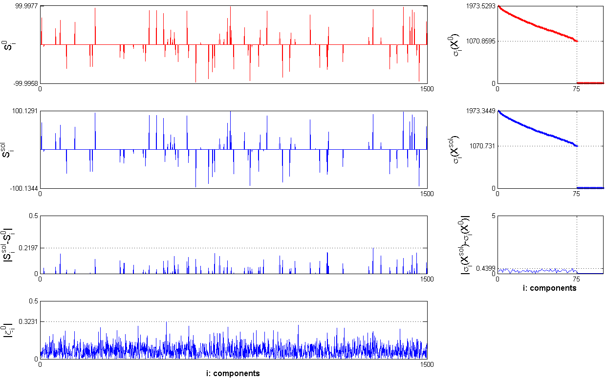
Table 5 shows that for all of the problem classes, the number of partial SVD required by ASALM was more than twice the number that NSA required. On the other hand, there was a big difference in CPU times; this difference can be explained by the fact that ASALM required more leading singular values than NSA did per partial SVD computation. Table 6 shows that although the relative errors of the low-rank components produced by NSA were slightly better, the relative errors of the sparse components produced by NSA were significantly better than those produced by ASALM. Finally, in Figure 1, we plot the decomposition of $D=X^{0}+S^{0}+\zeta^{0}\in\mathbb{R}^{n\times n}$ generated by NSA, where $\mathop{\operator@font rank}\nolimits(X^{0})=75$, $\|S^{0}\|_{0}=112,500$ and ${\rm SNR}(D)=45$. In the first row, we plot randomly selected 1500 components of $S^{0}$ and 100 leading singular values of $X^{0}$ in the first row. In the second row, we plot the same components of $S^{sol}$ and 100 singular of $X^{sol}$ produced by NSA. In the third row, we plot the absolute errors of $S^{sol}$ and $X^{sol}$. Note that the scales of the graphs showing absolute errors of $S^{sol}$ and $X^{sol}$ are larger than those of $S^{0}$ and $X^{0}$. And in the fourth row, we plot the same 1500 random components of $\zeta^{0}$. When we compare the absolute error graphs of $S^{sol}$ and $X^{sol}$ with the graph showing $\zeta^{0}$, we can confirm that the solution produced by NSA is inline with Theorem 2.

Table 5: NSA vs ASALM: Solution time for decomposing $D\in\mathbb{R}^{n\times n}$, $n=1500$

			$\mathbf{c_{r}}$=0.05 $\mathbf{c_{p}}$=0.05	$\mathbf{c_{r}}$=0.05 $\mathbf{c_{p}}$=0.1	$\mathbf{c_{r}}$=0.1 $\mathbf{c_{p}}$=0.05	$\mathbf{c_{r}}$=0.1 $\mathbf{c_{p}}$=0.1
SNR	Alg.	Field	min/avg/max	min/avg/max	min/avg/max	min/avg/max
$80dB$	$\mathbf{NSA}$	$\mathbf{SVD\#}$	10/10.0/10	10/10.9/11	12/12.0/12	12/12.2/13
		$\mathbf{CPU}$	38.6/44.1/46.6	43.7/48.6/51.9	78.6/84.1/90.8	80.7/97.7/155.2
	$\mathbf{ASALM}$	$\mathbf{SVD\#}$	22/22.0/22	20/20.0/20	29/29.0/29	29/29.4/30
		$\mathbf{CPU}$	657.3/677.8/736.2	809.7/850.0/874.7	1277.3/1316.1/1368.6	1833.2/1905.2/2004.7
$45dB$	$\mathbf{NSA}$	$\mathbf{SVD\#}$	7/7.9/8	8/8.0/8	9/9.0/9	9/9.0/9
		$\mathbf{CPU}$	34.1/37.7/44.0	30.7/37.1/45.6	55.6/59.0/63.7	55.9/59.7/64.8
	$\mathbf{ASALM}$	$\mathbf{SVD\#}$	21/21/21	18/18.5/19	28/28.0/28	27/27.3/28
		$\mathbf{CPU}$	666.6/686.9/708.9	835.7/857.1/887.2	1201.9/1223.2/1277.5	1677.1/1739.1/1846.5

Table 6: NSA vs ASALM: Solution accuracy for decomposing $D\in\mathbb{R}^{n\times n}$, $n=1500$

			$\mathbf{c_{r}}$=0.05 $\mathbf{c_{p}}$=0.05	$\mathbf{c_{r}}$=0.05 $\mathbf{c_{p}}$=0.1	$\mathbf{c_{r}}$=0.1 $\mathbf{c_{p}}$=0.05	$\mathbf{c_{r}}$=0.1 $\mathbf{c_{p}}$=0.1
SNR	Alg.	Relative Error	avg / max	avg / max	avg / max	avg / max
$80dB$	$\mathbf{NSA}$	$\mathbf{\frac{\|X^{sol}-X^{0}\|_{F}}{\|X^{0}\|_{F}}}$	1.8E-4 / 2.2E-4	2.1E-4 / 2.6E-4	1.3E-4 / 1.3E-4	2.8E-4 / 2.9E-4
		$\mathbf{\frac{\|S^{sol}-S^{0}\|_{F}}{\|S^{0}\|_{F}}}$	1.3E-4 / 1.6E-4	9.6E-5 / 1.1E-4	8.1E-5 / 8.5E-5	1.3E-4 / 1.4E-4
	$\mathbf{ASALM}$	$\mathbf{\frac{\|X^{sol}-X^{0}\|_{F}}{\|X^{0}\|_{F}}}$	3.9E-4 / 4.2E-4	8.4E-4 / 8.8E-4	6.6E-4 / 6.8E-4	1.4E-3 / 1.4E-3
		$\mathbf{\frac{\|S^{sol}-S^{0}\|_{F}}{\|S^{0}\|_{F}}}$	5.7E-4 / 6.2E-4	7.6E-4 / 8.0E-4	1.1E-3 / 1.1E-3	1.4E-3 / 1.4E-3
$45dB$	$\mathbf{NSA}$	$\mathbf{\frac{\|X^{sol}-X^{0}\|_{F}}{\|X^{0}\|_{F}}}$	3.4E-3 / 3.6E-3	4.7E-3 / 4.7E-3	3.9E-3 / 4.0E-3	5.3E-3 / 5.3E-3
		$\mathbf{\frac{\|S^{sol}-S^{0}\|_{F}}{\|S^{0}\|_{F}}}$	1.8E-3 / 1.8E-3	2.3E-3 / 2.3E-3	2.6E-3 / 3.5E-3	3.1E-3 / 3.1E-3
	$\mathbf{ASALM}$	$\mathbf{\frac{\|X^{sol}-X^{0}\|_{F}}{\|X^{0}\|_{F}}}$	4.6E-3 / 4.8E-3	7.3E-3 / 8.4E-3	4.7E-3 / 4.7E-3	7.8E-3 / 7.9E-3
		$\mathbf{\frac{\|S^{sol}-S^{0}\|_{F}}{\|S^{0}\|_{F}}}$	4.8E-3 / 4.9E-3	5.8E-3 / 7.0E-3	5.5E-3 / 5.5E-3	7.3E-3 / 7.5E-3

Fig. 1: NSA: Comparison of randomly selected 1500 components of $\zeta^{0}$ with absolute errors of those components in $S^{sol}$ and $\sigma(X^{sol})$. $D\in\mathbb{R}^{n\times n}$, $n=1500$, ${\rm SNR}(D)=45dB$

6.2 Foreground Detection on a Noisy Video

We used NSA and ASALM to extract moving objects in an airport security video [5], which is a sequence of 201 grayscale frames of size $144\times 176$. We assume that the airport security video [5] was not corrupted by Gaussian noise. We formed the $i$-th column of the data matrix $D$ by stacking the columns of the $i^{th}$ frame into a long vector, i.e. $D$ is in $\mathbb{R}^{25344\times 201}$. In order to have a noisy video with $\textnormal{SNR}=20dB$ signal-to-noise ratio (SNR), given $D$, we chose $\varrho=\|D\|_{F}/(\sqrt{144\times 176\times 201}~{}10^{\textnormal{SNR}/20})$ and then obtained a noisy $D$ by $D=D+\varrho~{}randn(144*176,201)$, where $randn(m,n)$ produces a random matrix with independent standard Gaussian entries. Solving for $(X^{*},S^{*})=\mathop{\rm argmin}_{X,S\in\mathbb{R}^{25344\times 201}}\{\|X\|_{*}+\xi\|S\|_{1}:\ \|X+S-D\|_{F}\leq\delta\}$, we decompose $D$ into a low rank matrix $X^{*}$ and a sparse matrix $S^{*}$. We estimate the $i$-th frame background image with the $i$-th column of $X^{*}$ and estimate the $i$-th frame moving object with the $i$-th column of $S^{*}$. Both algorithms are terminated when $\frac{\|(X_{k+1},S_{k+1})-(X_{k},S_{k})\|_{F}}{\|(X_{k},S_{k})\|_{F}+1}\leq\varrho\times 10^{-4}$.

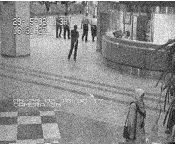
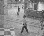
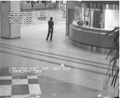
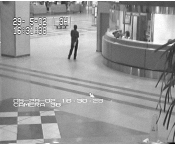
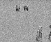
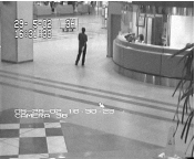
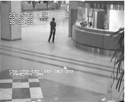
The recovery statistics of each algorithm are are displayed in Table 7. $(X^{sol},S^{sol})$ denote the variables corresponding to the low-rank and sparse components of $D$, respectively, when the algorithm of interest terminates. Figure 2 and Figure 3 show the $35$-th, $100$-th and $125$-th frames of the noise added airport security video [5] in their first row of images. The second and third rows in these tables have the recovered background and foreground images of the selected frames, respectively. Even though the visual quality of recovered background and foreground are very similar, Table 7 shows that both the number of partial SVDs and the CPU time of NSA are significantly less than those for ASALM.

Table 7: NSA vs ASALM: Recovery statistics for foreground detection on a noisy video

Alg.	$\mathbf{CPU}$	$\mathbf{SVD\#}$	$\mathbf{\|X^{sol}\|_{*}}$	$\mathbf{\|S^{sol}\|_{1}}$	$\mathop{\bf rank}(X^{sol})$	$\mathbf{\frac{\|X^{sol}+S^{sol}-D\|_{F}}{\|D\|_{F}}}$
$\mathbf{NSA}$	160.8	19	398662.9	76221854.1	81	0.00068
$\mathbf{ASALM}$	910.0	94	401863.6	75751977.1	89	0.00080

7 Acknowledgements

We would like to thank to Min Tao for providing the code ASALM.

    $D(t)$:
$X^{sol}(t)$:
$S^{sol}(t)$:

Fig. 2: Background extraction from a video with 20dB SNR using NSA

    $D(t)$:
$X^{sol}(t)$:
$S^{sol}(t)$:

Fig. 3: Background extraction from a video with 20dB SNR using ASALM

Appendix A Proof of Theorem 6

Definition 9.

Let $\phi:\mathbb{R}^{m\times n}\rightarrow\mathbb{R}$ and $\psi:\mathbb{R}^{m\times n}\times\mathbb{R}^{m\times n}\rightarrow\mathbb{R}$ be closed convex functions and define

$$Q^{\phi}(Z,S|X):=\psi(Z,S)+\phi(X)+\langle\gamma^{\phi}(X),Z-X\rangle+\frac{\rho}{2}\|Z-X\|_{F}^{2},$$ (70)

$$Q^{\psi}(Z|X,S):=\phi(Z)+\psi(X,S)+\langle\gamma_{x}^{\psi}(X,S),Z-X\rangle+\frac{\rho}{2}\|Z-X\|_{F}^{2},$$ (71)

and

$$\left(p^{\phi}_{x}(X),p^{\phi}_{s}(X)\right):=\mathop{\rm argmin}_{Z,S\in\mathbb{R}^{m\times n}}Q^{\phi}(Z,S|X),$$ (72)

$$p^{\psi}(X,S):=\mathop{\rm argmin}_{Z\in\mathbb{R}^{m\times n}}Q^{\psi}(Z|X,S),$$ (73)

where $\gamma^{\phi}(X)$ is any subgradient in the subdifferential $\partial\phi$ at the point $X$ and $\Big{(}\gamma_{x}^{\psi}(X,S),\gamma_{s}^{\psi}(X,S)\Big{)}$ is any subgradient in the subdifferential $\partial\psi$ at the point $(X,S)$.

Lemma 10.

Let $\phi$, $\psi$, $Q^{\phi}$, $Q^{\psi}$, $p_{x}^{\phi}$, $p_{s}^{\phi}$, $p^{\psi}$, $\gamma^{\phi}$, $\gamma_{x}^{\psi}$, $\gamma_{s}^{\psi}$ be as given in Definition A.1. and $\Phi(X,S):=\phi(X)+\psi(X,S)$. Let $X^{0}\in\mathbb{R}^{m\times n}$ and define $\hat{X}:=p_{x}^{\phi}(X^{0})$ and $\hat{S}:=p_{s}^{\phi}(X^{0})$. If

$$\Phi(\hat{X},\hat{S})\leq Q^{\phi}(\hat{X},\hat{S}|X^{0}),$$ (74)

then for any $(X,S)\in\mathbb{R}^{m\times n}\times\mathbb{R}^{m\times n}$,

$$\frac{2}{\rho}\left(\Phi(X,S)-\Phi\left(\hat{X},\hat{S}\right)\right)\geq\|X-\hat{X}\|_{F}^{2}-\|X-X^{0}\|_{F}^{2}.$$ (75)

Moreover, if

$$\Phi\left(p^{\psi}\left(\hat{X},\hat{S}\right),\hat{S}\right)\leq Q^{\psi}\left(p^{\psi}\left(\hat{X},\hat{S}\right)\Big{|}~{}\hat{X},\hat{S}\right),$$ (76)

then for any $(X,S)\in\mathbb{R}^{m\times n}\times\mathbb{R}^{m\times n}$,

$$\frac{2}{\rho}\Bigg{(}\Phi(X,S)-\Phi\Big{(}p^{\psi}\left(\hat{X},\hat{S}\right),\hat{S}\Big{)}\Bigg{)}\geq\|X-p^{\psi}\left(\hat{X},\hat{S}\right)\|_{F}^{2}-\|X-\hat{X}\|_{F}^{2}.$$ (77)

Proof.

Let $X^{0}\in\mathbb{R}^{m\times n}$ satisfy (74). Then for any $(X,S)\in\mathbb{R}^{m\times n}\times\mathbb{R}^{m\times n}$, we have

$$\Phi(X,S)-\Phi\left(p^{\phi}_{x}(X^{0}),\hat{S}\right) \geq\Phi(X,S)-Q^{\phi}\left(\hat{X},\hat{S}|X^{0}\right).$$ (78)

First order optimality conditions for (72) and $\psi$ being a closed convex function guarantee that there exists $\Bigg{(}\gamma^{\psi}_{x}\Big{(}\hat{X},\hat{S}\Big{)},\gamma^{\psi}_{s}\Big{(}\hat{X},\hat{S}\Big{)}\Bigg{)}\in\partial\psi\Big{(}\hat{X},\hat{S}\Big{)}$ such that

$$\gamma^{\psi}_{x}\Big{(}\hat{X},\hat{S}\Big{)}+\gamma^{\phi}(X^{0})+\rho\Big{(}\hat{X}-X^{0}\Big{)}=0,$$ (79)

$$\gamma^{\psi}_{s}\Big{(}\hat{X},\hat{S}\Big{)}=0,$$ (80)

where $\partial\psi\Big{(}\hat{X},\hat{S}\Big{)}$ denotes the subdifferential of $\psi(.,.)$ at the point $\Big{(}\hat{X},\hat{S}\Big{)}$.

Moreover, using the convexity of $\psi(.,.)$ and $\phi(.)$, we have

$$\psi(X,S)\geq\psi\Big{(}\hat{X},\hat{S}\Big{)}+\Big{\langle}\gamma^{\psi}_{x}\Big{(}\hat{X},\hat{S}\Big{)},X-\hat{X}\Big{\rangle}+\Big{\langle}\gamma^{\psi}_{s}\Big{(}\hat{X},\hat{S}\Big{)},S-\hat{S}\Big{\rangle},$$

$$\phi(X)\geq\phi(X^{0})+\langle\gamma^{\phi}(X^{0}),X-X^{0}\rangle.$$

These two inequalities and (80) together imply

$$\Phi(X,S)\geq\psi\Big{(}\hat{X},\hat{S}\Big{)}+\Big{\langle}\gamma^{\psi}_{x}\Big{(}\hat{X},\hat{S}\Big{)},X-\hat{X}\Big{\rangle}+\phi(X^{0})+\Big{\langle}\gamma^{\phi}(X^{0}),X-X^{0}\Big{\rangle}.$$ (81)

This inequality together with (74) and (79) gives

$$\Phi(X,S)-\Phi\Big{(}\hat{X},\hat{S}\Big{)}$$

$$\geq \Big{\langle}\gamma^{\psi}_{x}\Big{(}\hat{X},\hat{S}\Big{)},X-\hat{X}\Big{\rangle}+\Big{\langle}\gamma^{\phi}(X^{0}),X-X^{0}\Big{\rangle}-\Big{\langle}\gamma^{\phi}(X^{0}),\hat{X}-X^{0}\Big{\rangle}-\frac{\rho}{2}\|X-X^{0}\|_{F}^{2},$$

$$= \Big{\langle}\gamma^{\phi}(X^{0})+\gamma^{\psi}_{x}\Big{(}\hat{X},\hat{S}\Big{)},\ X-\hat{X}\Big{\rangle}-\frac{\rho}{2}\|X-X^{0}\|_{F}^{2},$$

$$= \rho~{}\Big{\langle}X^{0}-\hat{X},\ X-\hat{X}\Big{\rangle}-\frac{\rho}{2}\|X-X^{0}\|_{F}^{2},$$

$$= \frac{\rho}{2}\Big{(}\|X-\hat{X}\|_{F}^{2}-\|X-X^{0}\|_{F}^{2}\Big{)}.$$

Hence, we have (75). Suppose that $X^{0}$ satisfies (76). Then for any $(X,S)\in\mathbb{R}^{m\times n}\times\mathbb{R}^{m\times n}$, we have

$$\Phi(X,S)-\Phi\Big{(}p^{\psi}\left(\hat{X},\hat{S}\right),\hat{S}\Big{)} \geq\Phi(X,S)-Q^{\psi}\left(p^{\psi}\left(\hat{X},\hat{S}\right)|~{}\hat{X},\hat{S}\right).$$ (82)

First order optimality conditions for (73) and $\phi$ being a closed convex function guarantee that there exists $\gamma^{\phi}\Big{(}p^{\psi}\left(\hat{X},\hat{S}\right)\Big{)}\in\partial\phi\Big{(}p^{\psi}\left(\hat{X},\hat{S}\right)\Big{)}$ such that

$$\gamma^{\phi}\Big{(}p^{\psi}\left(\hat{X},\hat{S}\right)\Big{)}+\gamma_{x}^{\psi}\Big{(}\hat{X},\hat{S}\Big{)}+\rho\Big{(}p^{\psi}\left(\hat{X},\hat{S}\right)-\hat{X}\Big{)}=0.$$ (83)

Moreover, using the convexity of $\phi(.)$ and $\psi(.,.)$, we have

$$\phi(X)\geq\phi\Big{(}p^{\psi}\left(\hat{X},\hat{S}\right)\Big{)}+\Big{\langle}\gamma^{\phi}\Big{(}p^{\psi}\left(\hat{X},\hat{S}\right)\Big{)},X-p^{\psi}\left(\hat{X},\hat{S}\right)\Big{\rangle},$$ (84)

$$\psi(X,S)\geq\psi\Big{(}\hat{X},\hat{S}\Big{)}+\Big{\langle}\gamma^{\psi}_{x}\left(\hat{X},\hat{S}\right),X-\hat{X}\Big{\rangle},$$ (85)

where (85) follows from the fact that $\left(\hat{X},\hat{S}\right)=\mathop{\rm argmin}_{X,S}Q^{\phi}(X,S|~{}X^{0})$ implies $\left(\gamma^{\psi}_{x}\left(\hat{X},\hat{S}\right),~{}0\right)\in\partial\psi\left(\hat{X},\hat{S}\right)$, i.e. we can set $\gamma^{\psi}_{s}\left(\hat{X},\hat{S}\right)=0$. Summing the two inequalities (84) and (85) give

$$\Phi(X,S)\geq \ \psi\left(\hat{X},\hat{S}\right)+\Big{\langle}\gamma^{\psi}_{x}\left(\hat{X},\hat{S}\right),X-\hat{X}\Big{\rangle}+\phi\left(p^{\psi}\left(\hat{X},\hat{S}\right)\right)+\Big{\langle}\gamma^{\phi}\left(p^{\psi}\left(\hat{X},\hat{S}\right)\right),X-p^{\psi}\left(\hat{X},\hat{S}\right)\Big{\rangle}.$$ (86)

This inequality together with (76) and (83) gives

$$\Phi(X,S)-\Phi\Big{(}p^{\psi}\left(\hat{X},\hat{S}\right),\hat{S}\Big{)}$$

$$\geq \Big{\langle}\gamma^{\psi}_{x}(\hat{X},\hat{S}),X-\hat{X}\Big{\rangle}+\Big{\langle}\gamma^{\phi}\Big{(}p^{\psi}\left(\hat{X},\hat{S}\right)\Big{)},~{}X-p^{\psi}\left(\hat{X},\hat{S}\right)\Big{\rangle}$$

$$-\Big{\langle}\gamma_{x}^{\psi}\Big{(}\hat{X},\hat{S}\Big{)},~{}p^{\psi}\Big{(}\hat{X},\hat{S}\Big{)}-\hat{X}\Big{\rangle}-\frac{\rho}{2}\|p^{\psi}\Big{(}\hat{X},\hat{S}\Big{)}-\hat{X}\|_{F}^{2},$$

$$= \Big{\langle}\gamma^{\phi}\Big{(}p^{\psi}\left(\hat{X},\hat{S}\right)\Big{)}+\gamma^{\psi}_{x}\Big{(}\hat{X},\hat{S}\Big{)},\ X-p^{\psi}\left(\hat{X},\hat{S}\right)\Big{\rangle}-\frac{\rho}{2}\|p^{\psi}\left(\hat{X},\hat{S}\right)-\hat{X}\|_{F}^{2},$$

$$= \rho~{}\Big{\langle}\hat{X}-p^{\psi}\left(\hat{X},\hat{S}\right),\ X-p^{\psi}\left(\hat{X},\hat{S}\right)\Big{\rangle}-\frac{\rho}{2}\|p^{\psi}\left(\hat{X},\hat{S}\right)-\hat{X}\|_{F}^{2},$$

$$= \frac{\rho}{2}\left(\|X-p^{\psi}\left(\hat{X},\hat{S}\right)\|_{F}^{2}-\|X-\hat{X}\|_{F}^{2}\right).$$

Hence, we have (77). ∎

We are now ready to give the proof of Theorem 6.

Proof.

Let $I:=\{0\leq i\leq k-1:\Phi(X_{i+1},S_{i})\leq\mathcal{L}_{\rho}(X_{i+1},Z_{i},S_{i};Y_{i})\}$ and $I^{c}:=\{0,1,...,k-1\}\setminus I$. Since $\nabla\phi(.)$ is Lipschitz continuous with Lipschitz constant $L$ and $\rho\geq L$, $\Phi(p^{\phi}_{x}(X),p^{\phi}_{s}(X))\leq Q^{\phi}(p^{\phi}_{x}(X),p^{\phi}_{s}(X)|~{}X)$ is true for all $X\in\mathbb{R}^{m\times n}$. Since (74) in Lemma 10 is true for all $X^{0}\in\mathbb{R}^{m\times n}$, (75) is true for all $(X,S)\in\mathbb{R}^{m\times n}\times\mathbb{R}^{m\times n}$. Particularly, since for all $i\in I\cup I^{c}$

$$(Z_{i+1},S_{i+1})=\mathop{\rm argmin}_{Z,S}Q^{\phi}(Z,S|~{}X_{i+1}),$$ (87)

setting $(X,S):=(X^{*},S^{*})$ and $X^{0}:=X_{i+1}$ in Lemma 10 imply that $p^{\phi}_{x}(X_{i+1})=Z_{i+1}$, $p^{\phi}_{s}(X_{i+1})=S_{i+1}$ and we have

$$\frac{2}{\rho}\left(\Phi(X^{*},S^{*})-\Phi(Z_{i+1},S_{i+1})\right)\geq\|Z_{i+1}-X^{*}\|_{F}^{2}-\|X_{i+1}-X^{*}\|_{F}^{2}.$$ (88)

Moreover, (87) implies that for all $i\in I\cup I^{c}$, there exits $\left(\gamma^{\psi}_{x}(Z_{i},S_{i}),\gamma^{\psi}_{s}(Z_{i},S_{i})\right)\in\partial\psi(Z_{i},S_{i})$ such that

$$\gamma^{\psi}_{x}(Z_{i},S_{i})+\nabla\phi(X_{i})+\rho(Z_{i}-X_{i})=0,$$ (89)

$$\gamma^{\psi}_{s}(Z_{i},S_{i})=0.$$ (90)

(89) and the definition of $Y_{i+1}$ of Algorithm ALM-S shown in Algorithm 3 imply that

$$\gamma^{\psi}_{x}(Z_{i},S_{i})=-\nabla\phi(X_{i})+\rho(X_{i}-Z_{i})=Y_{i}.$$

Hence, by defining $Q^{\psi}(.|~{}Z_{i},S_{i})$ according to (71) using $\gamma^{\psi}_{x}(Z_{i},S_{i})=Y_{i}$, for all $X\in\mathbb{R}^{m\times n}$ we have

$$\mathcal{L}_{\rho}(X,Z_{i},S_{i};Y_{i})=\phi(X)+\psi(Z_{i},S_{i})+\langle Y_{i},X-Z_{i}\rangle+\frac{\rho}{2}\|X-Z_{i}\|_{F}^{2}=Q^{\psi}(X|~{}Z_{i},S_{i}).$$ (91)

for all $i\in I\cup I^{c}$. Hence, for all $i\in I$ $X_{i+1}=\mathop{\rm argmin}_{X}\mathcal{L}_{\rho}(X,Z_{i},S_{i};Y_{i})=\mathop{\rm argmin}_{X}Q^{\psi}(X|Z_{i},S_{i})$. Thus, for all $i\in I$, setting $X^{0}:=X_{i}$ in Lemma 10 imply $p^{\phi}_{x}(X_{i})=Z_{i}$, $p^{\phi}_{s}(X_{i})=S_{i}$ and $p^{\psi}(p^{\phi}_{x}(X_{i}),p^{\phi}_{s}(X_{i}))=p^{\psi}(Z_{i},S_{i})=X_{i+1}$. For all $i\in I$ we have $\Phi(X_{i+1},S_{i})\leq\mathcal{L}_{\rho}(X_{i+1},Z_{i},S_{i};Y_{i})=Q^{\psi}(X_{i+1}|Z_{i},S_{i})$. Hence, for all $i\in I$ setting $X^{0}:=X_{i}$ in Lemma 10 satisfies (76). Therefore, setting $(X,S):=(X^{*},S^{*})$ and $X^{0}:=X_{i}$ in Lemma 10 implies that

$$\frac{2}{\rho}\left(\Phi(X^{*},S^{*})-\Phi(X_{i+1},S_{i})\right)\geq\|X_{i+1}-X^{*}\|_{F}^{2}-\|Z_{i}-X^{*}\|_{F}^{2}.$$ (92)

For any $i\in I$, summing (88) and (92) gives

$$\frac{2}{\rho}\left(2\Phi(X^{*},S^{*})-\Phi(X_{i+1},S_{i})-\Phi(Z_{i+1},S_{i+1})\right)\geq\|Z_{i+1}-X^{*}\|_{F}^{2}-\|Z_{i}-X^{*}\|_{F}^{2}.$$ (93)

Moreover, since $X_{i+1}=Z_{i}$ for $i\in I^{c}$ and (88) holds for all $i\in I\cup I^{c}$, we trivially have

$$\frac{2}{\rho}\left(\Phi(X^{*},S^{*})-\Phi(Z_{i+1},S_{i+1})\right)\geq\|Z_{i+1}-X^{*}\|_{F}^{2}-\|Z_{i}-X^{*}\|_{F}^{2}.$$ (94)

Summing (93) and (94) over $i=0,1,...,k-1$ gives

$$\frac{2}{\rho}\left(\left(2|I|+|I^{c}|\right)\Phi(X^{*},S^{*})-\sum_{i\in I}\Phi(X_{i+1},S_{i})-\sum_{i=0}^{k-1}\Phi(Z_{i+1},S_{i+1})\right)\geq\|Z_{k}-X^{*}\|_{F}^{2}-\|Z_{0}-X^{*}\|_{F}^{2}.$$ (95)

For any $i\in I\cup I^{c}$, setting $(X,S):=(X_{i+1},S_{i})$ and $X^{0}:=X_{i+1}$ in Lemma 10 gives

$$\frac{2}{\rho}\left(\Phi(X_{i+1},S_{i})-\Phi(Z_{i+1},S_{i+1})\right)\geq\|Z_{i+1}-X_{i+1}\|_{F}^{2}\geq 0.$$ (96)

Trivially, for $i=1,...,k$ we also have

$$\frac{2}{\rho}\left(\Phi(X_{i},S_{i-1})-\Phi(Z_{i},S_{i})\right)\geq\|Z_{i}-X_{i}\|_{F}^{2}\geq 0.$$ (97)

Moreover, since for all $i\in I$ setting $X^{0}:=X_{i}$ in Lemma 10 satisfies (76), setting $(X,S):=(Z_{i},S_{i})$ and $X^{0}:=X_{i}$ in Lemma 10 implies that

$$\frac{2}{\rho}\left(\Phi(Z_{i},S_{i})-\Phi(X_{i+1},S_{i})\right)\geq\|X_{i+1}-Z_{i}\|_{F}^{2}\geq 0.$$ (98)

And since $X_{i+1}=Z_{i}$ for all $i\in I^{c}$, (98) trivially holds for all $i\in I^{c}$. Thus, for all $i\in I\cup I^{c}$ we have

$$\frac{2}{\rho}\left(\Phi(Z_{i},S_{i})-\Phi(X_{i+1},S_{i})\right)\geq 0.$$ (99)

Adding (96) and (99) yields $\Phi(Z_{i},S_{i})\geq\Phi(Z_{i+1},S_{i+1})$ for all $i\in I\cup I^{c}$ and adding (97) and (99) yields $\Phi(X_{i},S_{i-1})\geq\Phi(X_{i+1},S_{i})$ for all $i=1,...,k-1$. Hence,

$$\sum_{i=0}^{k-1}\Phi(Z_{i+1},S_{i+1})\geq k\Phi(Z_{k},S_{k}),\mbox{ and }\sum_{i\in I}\Phi(X_{i+1},S_{i})\geq n_{k}\Phi(X_{k},S_{k-1}).$$ (100)

These two inequalities, (95) and the fact that $X_{0}=Z_{0}$ imply

$$\frac{2}{\rho}\left(\left(2|I|+|I^{c}|\right)\Phi(X^{*},S^{*})-n_{k}\Phi(X_{k},S_{k-1})-k\Phi(Z_{k},S_{k})\right)\geq-\|X_{0}-X^{*}\|_{F}^{2}.$$ (101)

Hence, (50) follows from the facts: $2|I|+|I^{c}|=k+n_{k}$ and $n_{k}\Phi(X_{k},S_{k-1})+k\Phi(Z_{k},S_{k})\geq(k+n_{k})\Phi(Z_{k},S_{k})$ due to (96). ∎

Appendix B Proof of Lemma 7

Proof.

Since $Y^{*}$ and $\theta^{*}$ are optimal Lagrangian dual variables, we have

$$(X^{*},X^{*},S^{*})=\mathop{\rm argmin}_{X,Z,S}\|X\|_{*}+\xi~{}\|S\|_{1}+\langle Y^{*},X-Z\rangle+\frac{\theta^{*}}{2}\left(\|Z+S-D\|^{2}_{F}-\delta^{2}\right).$$

Then from first-order optimality conditions, we have

$$0\in\partial\|X^{*}\|_{*}+Y^{*},$$

$$0\in\xi~{}\partial\|S^{*}\|_{1}+\theta^{*}(X^{*}+S^{*}-D),$$

$$-Y^{*}+\theta^{*}(X^{*}+S^{*}-D)=0.$$

Hence, $-Y^{*}\in\partial\|X^{*}\|_{*}$ and $-Y^{*}\in\xi~{}\partial\|S^{*}\|_{1}$.

For $k\geq 0$, since $X_{k+1}$ is the optimal solution for the $k$-th subproblem given in Step 4 in Algorithm 5, from the first-order optimality conditions it follows that

$$0\in\partial\|X_{k+1}\|_{*}+Y_{k}+\rho_{k}(X_{k+1}-Z_{k}).$$ (102)

For $k\geq 0$, let $\theta_{k}\geq 0$ be the optimal Lagrange multiplier for the quadratic constraint in the $k$-th subproblem given in Step 6 in Algorithm 5. Since $(S_{k+1},Z_{k+1})$ is the optimal solution, from the first-order optimality conditions it follows that

$$0\in\xi\partial\|S_{k+1}\|_{1}+\theta_{k}(Z_{k+1}+S_{k+1}-D),$$ (103)

$$-Y_{k}+\rho_{k}(Z_{k+1}-X_{k+1})+\theta_{k}(Z_{k+1}+S_{k+1}-D)=0.$$ (104)

From (102), it follows that $-\hat{Y}_{k+1}\in\partial\|X_{k+1}\|_{*}$. Hence, $\{\hat{Y}_{k}\}_{k\in\mathbb{Z}_{+}}$ is a bounded sequence. From (103) and (104), it follows that $-Y_{k+1}\in\xi~{}\partial\|S_{k+1}\|_{1}$. Hence, $\{Y_{k}\}_{k\in\mathbb{Z}_{+}}$ is also a bounded sequence.

Furthermore, since $Y_{k+1}-Y_{k}=\rho_{k}(X_{k+1}-Z_{k+1})$ and $Y_{k+1}-\hat{Y}_{k+1}=\rho_{k}(Z_{k}-Z_{k+1})$, we have

$$\rho_{k}^{-1}\langle Y_{k+1}-Y_{k},Y_{k+1}-Y^{*}\rangle$$

$$= \langle X_{k+1}-Z_{k+1},Y_{k+1}-Y^{*}\rangle,$$

$$= \langle X_{k+1}-X^{*},Y_{k+1}-Y^{*}\rangle+\langle X^{*}-Z_{k+1},Y_{k+1}-Y^{*}\rangle,$$

$$= \langle X_{k+1}-X^{*},Y_{k+1}-\hat{Y}_{k+1}\rangle+\langle X_{k+1}-X^{*},\hat{Y}_{k+1}-Y^{*}\rangle+\langle X^{*}-Z_{k+1},Y_{k+1}-Y^{*}\rangle,$$

$$= \rho_{k}\langle X_{k+1}-X^{*},Z_{k}-Z_{k+1}\rangle+\langle X_{k+1}-X^{*},\hat{Y}_{k+1}-Y^{*}\rangle+\langle X^{*}-Z_{k+1},Y_{k+1}-Y^{*}\rangle.$$

Using the above equality, for all $k\geq 1$, we trivially have

$$\|Z_{k+1}-X^{*}\|_{F}^{2}+\rho_{k}^{-2}\|Y_{k+1}-Y^{*}\|_{F}^{2}$$

$$= \|Z_{k}-X^{*}\|_{F}^{2}+\rho_{k}^{-2}\|Y_{k}-Y^{*}\|_{F}^{2}-\|Z_{k+1}-Z_{k}\|_{F}^{2}-\rho_{k}^{-2}\|Y_{k+1}-Y_{k}\|_{F}^{2},$$

$$+2\langle Z_{k+1}-X^{*},Z_{k+1}-Z_{k}\rangle+2\rho_{k}^{-2}\langle Y_{k+1}-Y_{k},Y_{k+1}-Y^{*}\rangle,$$

$$= \|Z_{k}-X^{*}\|_{F}^{2}+\rho_{k}^{-2}\|Y_{k}-Y^{*}\|_{F}^{2}-\|Z_{k+1}-Z_{k}\|_{F}^{2}-\rho_{k}^{-2}\|Y_{k+1}-Y_{k}\|_{F}^{2},$$

$$+2\langle Z_{k+1}-X^{*},Z_{k+1}-Z_{k}\rangle+2\langle X_{k+1}-X^{*},Z_{k}-Z_{k+1}\rangle$$

$$-2\rho_{k}^{-1}\left(\langle-\hat{Y}_{k+1}+Y^{*},X_{k+1}-X^{*}\rangle+\langle-Y_{k+1}+Y^{*},X^{*}-Z_{k+1}\rangle\right)$$

$$= \|Z_{k}-X^{*}\|_{F}^{2}+\rho_{k}^{-2}\|Y_{k}-Y^{*}\|_{F}^{2}-\|Z_{k+1}-Z_{k}\|_{F}^{2}-\rho_{k}^{-2}\|Y_{k+1}-Y_{k}\|_{F}^{2},$$

$$+2\langle Z_{k+1}-X_{k+1},Z_{k+1}-Z_{k}\rangle-2\rho_{k}^{-1}\left(\langle-\hat{Y}_{k+1}+Y^{*},X_{k+1}-X^{*}\rangle+\langle-Y_{k+1}+Y^{*},X^{*}-Z_{k+1}\rangle\right)$$

$$= \|Z_{k}-X^{*}\|_{F}^{2}+\rho_{k}^{-2}\|Y_{k}-Y^{*}\|_{F}^{2}-\|Z_{k+1}-Z_{k}\|_{F}^{2}-\rho_{k}^{-2}\|Y_{k+1}-Y_{k}\|_{F}^{2},$$

$$-2\rho_{k}^{-1}\left(\langle Y_{k+1}-Y_{k},Z_{k+1}-Z_{k}\rangle+\langle-\hat{Y}_{k+1}+Y^{*},X_{k+1}-X^{*}\rangle+\langle-Y_{k+1}+Y^{*},X^{*}-Z_{k+1}\rangle\right)$$ (105)

Since $-Y_{k}\in\xi~{}\partial\|S_{k}\|_{1}$ for all $k\geq 1$ and $-Y^{*}\in\xi~{}\partial\|S^{*}\|_{1}$, we have for all $k\geq 1$

$$\langle-Y_{k+1}+Y_{k},S_{k+1}-S_{k}\rangle\geq 0,$$ (106)

$$\langle-Y_{k+1}+Y^{*},S_{k+1}-S^{*}\rangle\geq 0.$$ (107)

Since $\rho_{k+1}\geq\rho_{k}$ for all $k\geq 1$, adding (106), (107) to (105) and subtracting (107) from (105), we have

$$\|Z_{k+1}-X^{*}\|_{F}^{2}+\rho_{k+1}^{-2}\|Y_{k+1}-Y^{*}\|_{F}^{2}$$

$$\leq~{} \|Z_{k+1}-X^{*}\|_{F}^{2}+\rho_{k}^{-2}\|Y_{k+1}-Y^{*}\|_{F}^{2}$$

$$\leq~{} \|Z_{k}-X^{*}\|_{F}^{2}+\rho_{k}^{-2}\|Y_{k}-Y^{*}\|_{F}^{2}-\|Z_{k+1}-Z_{k}\|_{F}^{2}-\rho_{k}^{-2}\|Y_{k+1}-Y_{k}\|_{F}^{2}$$

$$-2\rho_{k}^{-1}\left(\langle-\hat{Y}_{k+1}+Y^{*},X_{k+1}-X^{*}\rangle+\langle-Y_{k+1}+Y^{*},S_{k+1}-S^{*}\rangle\right)$$

$$-2\rho_{k}^{-1}\left(\langle Y_{k+1}-Y_{k},Z_{k+1}+S_{k+1}-Z_{k}-S_{k}\rangle+\langle-Y_{k+1}+Y^{*},X^{*}+S^{*}-Z_{k+1}-S_{k+1}\rangle\right)$$ (108)

Applying Lemma 5 on the $k$-th subproblem given in Step 6 in Algorithm 5, it follows that

$$(Y_{k+1},Y_{k+1})\in\partial\mathbf{1}_{\chi}(Z_{k+1},S_{k+1}).$$

Using arguments similar to those used in the proof of Lemma 5, one can also show that

$$(Y^{*},Y^{*})\in\partial\mathbf{1}_{\chi}(X^{*},S^{*}).$$

Moreover, since $-Y_{k}\in\xi~{}\partial\|S_{k}\|_{1}$, $-\hat{Y}_{k}\in\xi~{}\partial\|X_{k}\|_{*}$ for all $k\geq 1$, $-Y^{*}\in\xi~{}\partial\|S^{*}\|_{1}$ and $-Y^{*}\in\partial\|X^{*}\|_{*}$, we have

$$\langle Y_{k+1}-Y_{k},Z_{k+1}+S_{k+1}-Z_{k}-S_{k}\rangle\geq 0,$$

$$\langle-Y_{k+1}+Y^{*},X^{*}+S^{*}-Z_{k+1}-S_{k+1}\rangle\geq 0,$$

$$\langle-Y_{k+1}+Y^{*},S_{k+1}-S^{*}\rangle\geq 0,$$

$$\langle-\hat{Y}_{k+1}+Y^{*},X_{k+1}-X^{*}\rangle\geq 0,$$

for all $k\geq 1$. Therefore, the above inequalities and (108) together imply that $\{\|Z_{k}-X^{*}\|_{F}^{2}+\rho_{k}^{-2}\|Y_{k}-Y^{*}\|_{F}^{2}\}_{k\in\mathbb{Z}_{+}}$ is a non-increasing sequence. Moreover, we also have

$$\sum_{k\in\mathbb{Z}_{+}}\|Z_{k+1}-Z_{k}\|_{F}^{2}+\rho_{k}^{-2}\|Y_{k+1}-Y_{k}\|_{F}^{2}$$

$$+ 2\sum_{k\in\mathbb{Z}_{+}}\rho_{k}^{-1}\left(\langle-\hat{Y}_{k+1}+Y^{*},X_{k+1}-X^{*}\rangle+\langle-Y_{k+1}+Y^{*},S_{k+1}-S^{*}\rangle\right)$$

$$+ 2\sum_{k\in\mathbb{Z}_{+}}\rho_{k}^{-1}\left(\langle Y_{k+1}-Y_{k},Z_{k+1}+S_{k+1}-Z_{k}-S_{k}\rangle+\langle-Y_{k+1}+Y^{*},X^{*}+S^{*}-Z_{k+1}-S_{k+1}\rangle\right)$$

$$= \sum_{k\in\mathbb{Z}_{+}}\left(\|Z_{k}-X^{*}\|_{F}^{2}+\rho_{k}^{-2}\|Y_{k}-Y^{*}\|_{F}^{2}-\|Z_{k+1}-X^{*}\|_{F}^{2}-\rho_{k+1}^{-2}\|Y_{k+1}-Y^{*}\|_{F}^{2}\right)<\infty$$

∎

Appendix C Additional Statistics for Numerical Experiments

Table 8: NSA vs ASALM: Additional statistics on solution accuracy for decomposing $D\in\mathbb{R}^{n\times n}$, $n=1500$, ${\rm SNR}(D)=80dB$

	$\mathbf{c_{r}}$=0.05 $\mathbf{c_{p}}$=0.05		$\mathbf{c_{r}}$=0.05 $\mathbf{c_{p}}$=0.1
	NSA	ASALM	NSA	ASALM
Error Type	avg / max	avg / max	avg / max	avg / max
$\mathbf{|~{}\|X^{sol}\|_{*}-\|X^{0}\|_{*}|/\|X^{0}\|_{*}}$	1.7E-6 /  5.2E-6	6.9E-6 /  1.0E-5	5.0E-6 /  3.2E-5	2.3E-5 /  3.8E-5
$\mathbf{\max\{|\sigma_{i}-\sigma^{0}_{i}|:\sigma^{0}_{i}>0\}}$	4.1E-2 /  5.2E-2	3.9E-2 /  4.7E-2	5.2E-2 /  1.8E-1	1.1E-1 /  1.7E-1
$\mathbf{\max\{|\sigma_{i}|:\sigma^{0}_{i}=0\}}$	7.9E-13 /  2.2E-12	6.3E-13 /  1.6E-12	8.6E-13 /  2.0E-12	1.1E-12 /  2.0E-12
$\mathbf{|~{}\|S^{sol}\|_{1}-\|S^{0}\|_{1}|/\|S^{0}\|_{1}}$	1.1E-5 /  1.4E-5	6.2E-6 /  9.7E-6	9.7E-6 /  1.5E-5	8.6E-5 /  9.7E-5
$\mathbf{\max\{|S^{sol}_{ij}-S^{0}_{ij}|:S^{0}_{ij}\neq 0\}}$	2.9E-1 /  3.5E-1	5.9E-1 /  8.0E-1	2.2E-1 /  2.4E-1	5.9E-1 /  7.4E-1
$\mathbf{\max\{|S^{sol}_{ij}|:S^{0}_{ij}=0\}}$	0 /  0	4.0E-1 /  7.2E-1	8.3E-3 /  1.1E-2	1.9E-1 /  5.5E-1
	$\mathbf{c_{r}}$=0.1 $\mathbf{c_{p}}$=0.05		$\mathbf{c_{r}}$=0.1 $\mathbf{c_{p}}$=0.1
	NSA	ASALM	NSA	ASALM
Error Type	avg / max	avg / max	avg / max	avg / max
$\mathbf{|~{}\|X^{sol}\|_{*}-\|X^{0}\|_{*}|/\|X^{0}\|_{*}}$	5.6E-6 /  6.4E-6	4.6E-5 /  4.9E-5	6.2E-6 /  7.1E-6	1.2E-4 /  1.4E-4
$\mathbf{\max\{|\sigma_{i}-\sigma^{0}_{i}|:\sigma^{0}_{i}>0\}}$	5.7E-2 /  6.2E-2	1.2E-1 /  1.3E-1	8.8E-2 /  1.0E-1	3.0E-1 /  3.7E-1
$\mathbf{\max\{|\sigma_{i}|:\sigma^{0}_{i}=0\}}$	6.9E-13 / 1.5E-12	6.2E-13 /  9.9E-13	6.2E-13 /  1.3E-12	3.9E-13 /  1.0E-12
$\mathbf{|~{}\|S^{sol}\|_{1}-\|S^{0}\|_{1}|/\|S^{0}\|_{1}}$	1.2E-5 /  1.6E-5	1.6E-4 /  1.7E-4	3.4E-5 /  3.7E-5	2.5E-4 /  2.7E-4
$\mathbf{\max\{|S^{sol}_{ij}-S^{0}_{ij}|:S^{0}_{ij}\neq 0\}}$	1.6E-1 /  1.9E-1	6.7E-1 /  8.3E-1	1.7E-1 /  2.0E-1	7.9E-1 /  9.5E-1
$\mathbf{\max\{|S^{sol}_{ij}|:S^{0}_{ij}=0\}}$	7.0E-3 /  1.1E-2	1.5E-1 /  2.5E-1	1.3E-2 /  1.9E-2	1.2E-1 /  2.5E-1

Table 9: NSA vs ASALM: Additional statistics on solution accuracy for decomposing $D\in\mathbb{R}^{n\times n}$, $n=1500$, ${\rm SNR}(D)=45dB$

	$\mathbf{c_{r}}$=0.05 $\mathbf{c_{p}}$=0.05		$\mathbf{c_{r}}$=0.05 $\mathbf{c_{p}}$=0.1
	NSA	ASALM	NSA	ASALM
Error Type	avg / max	avg / max	avg / max	avg / max
$\mathbf{|~{}\|X^{sol}\|_{*}-\|X^{0}\|_{*}|/\|X^{0}\|_{*}}$	1.8E-4 /  3.6E-4	1.4E-3 /  1.5E-3	2.2E-4 /  2.4E-4	2.4E-3 /  2.6E-3
$\mathbf{\max\{|\sigma_{i}-\sigma^{0}_{i}|:\sigma^{0}_{i}>0\}}$	5.9E-1 /  1.8E+0	1.1E+0 /  1.5E+0	9.8E-1 /  1.1E+0	2.3E+0 /  2.6E+0
$\mathbf{\max\{|\sigma_{i}|:\sigma^{0}_{i}=0\}}$	6.4E-13 /  1.3E-12	3.7E+0 / 3.8E+0	6.1E-13 / 1.0E-12	4.7E+0 / 5.5E+0
$\mathbf{|~{}\|S^{sol}\|_{1}-\|S^{0}\|_{1}|/\|S^{0}\|_{1}}$	1.7E-4 /  1.9E-4	4.2E-3 /  4.3E-3	1.3E-4 /  1.3E-4	2.9E-3 /  3.6E-3
$\mathbf{\max\{|S^{sol}_{ij}-S^{0}_{ij}|:S^{0}_{ij}\neq 0\}}$	1.0E+0 /  1.2E+0	3.0E+0 /  3.6E+0	1.3E+0 /  1.4E+0	3.2E+0 /  3.8E+0
$\mathbf{\max\{|S^{sol}_{ij}|:S^{0}_{ij}=0\}}$	3.6E-1 /  4.0E-1	2.2E+0 /  2.6E+0	5.3E-1 /  6.1E-1	2.3E+0 /  3.1E+0
	$\mathbf{c_{r}}$=0.1 $\mathbf{c_{p}}$=0.05		$\mathbf{c_{r}}$=0.1 $\mathbf{c_{p}}$=0.1
	NSA	ASALM	NSA	ASALM
Error Type	avg / max	avg / max	avg / max	avg / max
$\mathbf{|~{}\|X^{sol}\|_{*}-\|X^{0}\|_{*}|/\|X^{0}\|_{*}}$	3.7E-4 /  6.5E-4	9.7E-5 /  1.3E-4	6.7E-4 /  6.8E-4	8.4E-4 /  9.0E-4
$\mathbf{\max\{|\sigma_{i}-\sigma^{0}_{i}|:\sigma^{0}_{i}>0\}}$	1.3E+0 /  1.5E+0	1.2E+0 /  1.3E+0	2.5E+0 /  2.8E+0	1.3E+0 /  1.5E+0
$\mathbf{\max\{|\sigma_{i}|:\sigma^{0}_{i}=0\}}$	1.6E-1 /  1.6E+0	3.6E+0 /  3.7E+0	7.3E-13 /  1.7E-12	3.2E+0 /  3.3E+0
$\mathbf{|~{}\|S^{sol}\|_{1}-\|S^{0}\|_{1}|/\|S^{0}\|_{1}}$	8.1E-4 /  3.2E-3	4.7E-3 /  4.8E-3	8.9E-4 /  9.0E-4	4.4E-3 /  4.5E-3
$\mathbf{\max\{|S^{sol}_{ij}-S^{0}_{ij}|:S^{0}_{ij}\neq 0\}}$	9.3E-1 /  1.1E+0	2.7E+0 /  3.3E+0	1.1E+0 /  1.2E+0	3.2E+0 /  3.5E+0
$\mathbf{\max\{|S^{sol}_{ij}|:S^{0}_{ij}=0\}}$	5.7E-1 /  6.6E-1	1.1E+0 /  1.4E+0	7.1E-1 /  7.9E-1	1.3E+0 /  1.6E+0

Table 10: NSA: Additional statistics on solution accuracy for decomposing $D\in\mathbb{R}^{n\times n}$, $n\in\{500,1000,1500\}$, ${\rm SNR}(D)=80dB$

		$\mathbf{c_{r}}$=0.05 $\mathbf{c_{p}}$=0.05	$\mathbf{c_{r}}$=0.05 $\mathbf{c_{p}}$=0.1	$\mathbf{c_{r}}$=0.1 $\mathbf{c_{p}}$=0.05	$\mathbf{c_{r}}$=0.1 $\mathbf{c_{p}}$=0.1
n	Error Type	avg / max	avg / max	avg / max	avg / max
$\mathbf{500}$	$\mathbf{\frac{|~{}\|X^{sol}\|_{*}-\|X^{0}\|_{*}|}{\|X^{0}\|_{*}}}$	7.2E-6 /  1.1E-5	2.0E-5 /  2.7E-5	5.6E-6 /  8.2E-6	2.1E-5 /  3.1E-5
	$\mathbf{\max\{|\sigma_{i}-\sigma^{0}_{i}|:\sigma^{0}_{i}>0\}}$	1.7E-2 /  2.4E-2	3.4E-2 /  5.6E-2	2.1E-2 /  2.7E-2	3.2E-2 /  3.8E-2
	$\mathbf{\max\{|\sigma_{i}|:\sigma^{0}_{i}=0\}}$	1.6E-13 /  2.9E-13	2.0E-13 /  5.6E-13	1.1E-13 /  2.5E-13	8.6E-14 /  1.7E-13
	$\mathbf{\frac{|~{}\|S^{sol}\|_{1}-\|S^{0}\|_{1}|}{\|S^{0}\|_{1}}}$	1.6E-5 /  1.7E-5	1.5E-5 /  1.8E-5	2.9E-5 /  3.2E-5	2.6E-5 /  3.0E-5
	$\mathbf{\max\{|S^{sol}_{ij}-S^{0}_{ij}|:S^{0}_{ij}\neq 0\}}$	3.2E-1 /  4.0E-1	3.0E-1 /  4.3E-1	2.6E-1 /  3.2E-1	1.8E-1 /  2.3E-1
	$\mathbf{\max\{|S^{sol}_{ij}|:S^{0}_{ij}=0\}}$	9.5E-3 /  2.2E-2	1.5E-2 /  2.5E-2	1.5E-2 /  2.5E-2	1.8E-2 /  3.4E-2
$\mathbf{1000}$	$\mathbf{\frac{|~{}\|X^{sol}\|_{*}-\|X^{0}\|_{*}|}{\|X^{0}\|_{*}}}$	5.6E-6 /  1.7E-5	6.2E-6 /  1.7E-5	6.9E-6 /  8.6E-6	1.5E-6 /  2.6E-6
	$\mathbf{\max\{|\sigma_{i}-\sigma^{0}_{i}|:\sigma^{0}_{i}>0\}}$	1.8E-2 /  4.0E-2	3.1E-2 /  4.8E-2	5.1E-2 /  6.0E-2	5.9E-2 /  6.8E-2
	$\mathbf{\max\{|\sigma_{i}|:\sigma^{0}_{i}=0\}}$	3.3E-13 /  4.8E-13	3.3E-13 /  5.0E-13	2.9E-13 /  6.6E-13	2.8E-13 /  4.8E-13
	$\mathbf{\frac{|~{}\|S^{sol}\|_{1}-\|S^{0}\|_{1}|}{\|S^{0}\|_{1}}}$	1.1E-5 /  1.5E-5	1.7E-5 /  1.9E-5	2.8E-5 /  3.0E-5	2.9E-5 /  3.0E-5
	$\mathbf{\max\{|S^{sol}_{ij}-S^{0}_{ij}|:S^{0}_{ij}\neq 0\}}$	2.7E-1 /  3.1E-1	3.1E-1 /  3.8E-1	2.2E-1 /  2.8E-1	1.6E-1 /  1.7E-1
	$\mathbf{\max\{|S^{sol}_{ij}|:S^{0}_{ij}=0\}}$	1.7E-4 /  9.7E-4	1.2E-2 /  1.7E-2	7.8E-3 /  1.2E-2	1.2E-2 /  1.5E-2
$\mathbf{1500}$	$\mathbf{\frac{|~{}\|X^{sol}\|_{*}-\|X^{0}\|_{*}|}{\|X^{0}\|_{*}}}$	1.7E-6 /  5.2E-6	5.0E-6 /  3.2E-5	5.6E-6 /  6.4E-6	6.2E-6 /  7.1E-6
	$\mathbf{\max\{|\sigma_{i}-\sigma^{0}_{i}|:\sigma^{0}_{i}>0\}}$	4.1E-2 /  5.2E-2	5.2E-2 /  1.8E-1	5.7E-2 /  6.2E-2	8.8E-2 /  1.0E-1
	$\mathbf{\max\{|\sigma_{i}|:\sigma^{0}_{i}=0\}}$	7.9E-13 /  2.2E-12	8.6E-13 /  2.0E-12	6.9E-13 /  1.5E-12	6.2E-13 /  1.3E-12
	$\mathbf{\frac{|~{}\|S^{sol}\|_{1}-\|S^{0}\|_{1}|}{\|S^{0}\|_{1}}}$	1.1E-5 /  1.4E-5	9.7E-6 /  1.5E-5	1.2E-5 /  1.6E-5	3.4E-5 /  3.7E-5
	$\mathbf{\max\{|S^{sol}_{ij}-S^{0}_{ij}|:S^{0}_{ij}\neq 0\}}$	2.9E-1 /  3.5E-1	2.2E-1 /  2.4E-1	1.6E-1 /  1.9E-1	1.7E-1 /  2.0E-1
	$\mathbf{\max\{|S^{sol}_{ij}|:S^{0}_{ij}=0\}}$	0 /  0	8.3E-3 /  1.1E-2	7.0E-3 /  1.1E-2	1.3E-2 /  1.9E-2

Table 11: NSA: Additional statistics on solution accuracy for decomposing $D\in\mathbb{R}^{n\times n}$, $n\in\{500,1000,1500\}$, ${\rm SNR}(D)=45dB$

		$\mathbf{c_{r}}$=0.05 $\mathbf{c_{p}}$=0.05	$\mathbf{c_{r}}$=0.05 $\mathbf{c_{p}}$=0.1	$\mathbf{c_{r}}$=0.1 $\mathbf{c_{p}}$=0.05	$\mathbf{c_{r}}$=0.1 $\mathbf{c_{p}}$=0.1
n	Error Type	avg / max	avg / max	avg / max	avg / max
$\mathbf{500}$	$\mathbf{\frac{|~{}\|X^{sol}\|_{*}-\|X^{0}\|_{*}|}{\|X^{0}\|_{*}}}$	6.0E-4 /  9.3E-4	5.5E-4 /  6.2E-4	7.4E-4 /  8.8E-4	1.0E-3 /  1.3E-3
	$\mathbf{\max\{|\sigma_{i}-\sigma^{0}_{i}|:\sigma^{0}_{i}>0\}}$	5.1E-1 /  7.8E-1	5.4E-1 /  7.7E-1	8.2E-1 /  8.9E-1	9.2E-1 /  1.2E+0
	$\mathbf{\max\{|\sigma_{i}|:\sigma^{0}_{i}=0\}}$	1.7E-13 / 2.7E-13	1.6E-13 /  3.0E-13	1.0E-13 /  2.1E-13	1.1E-1 /  6.0E-1
	$\mathbf{\frac{|~{}\|S^{sol}\|_{1}-\|S^{0}\|_{1}|}{\|S^{0}\|_{1}}}$	3.0E-4 /  3.4E-4	2.1E-4 /  2.9E-4	3.0E-4 /  1.2E-3	6.4E-4 /  1.1E-3
	$\mathbf{\max\{|S^{sol}_{ij}-S^{0}_{ij}|:S^{0}_{ij}\neq 0\}}$	1.6E+0 /  1.9E+0	1.4E+0 /  1.8E+0	1.2E+0 /  1.6E+0	1.0E+0 /  1.3E+0
	$\mathbf{\max\{|S^{sol}_{ij}|:S^{0}_{ij}=0\}}$	2.3E-1 /  2.9E-1	4.0E-1 /  4.7E-1	3.5E-1 /  4.6E-1	5.4E-1 /  6.1E-1
$\mathbf{1000}$	$\mathbf{\frac{|~{}\|X^{sol}\|_{*}-\|X^{0}\|_{*}|}{\|X^{0}\|_{*}}}$	2.8E-4 /  3.1E-4	4.4E-4 /  7.5E-4	5.6E-4 /  8.0E-4	7.4E-4 /  8.4E-4
	$\mathbf{\max\{|\sigma_{i}-\sigma^{0}_{i}|:\sigma^{0}_{i}>0\}}$	5.2E-1 /  6.2E-1	8.6E-1 /  1.2E+0	1.7E+0 /  1.9E+0	1.8E+0 /  1.9E+0
	$\mathbf{\max\{|\sigma_{i}|:\sigma^{0}_{i}=0\}}$	2.5E-13 / 5.3E-13	4.3E-13 /  9.0E-13	2.0E-1 /  2.0E+0	6.3E-1 /  3.9E+0
	$\mathbf{\frac{|~{}\|S^{sol}\|_{1}-\|S^{0}\|_{1}|}{\|S^{0}\|_{1}}}$	2.2E-4 /  2.3E-4	1.4E-4 /  1.7E-4	5.5E-4 /  3.7E-3	1.1E-3 /  2.5E-3
	$\mathbf{\max\{|S^{sol}_{ij}-S^{0}_{ij}|:S^{0}_{ij}\neq 0\}}$	1.3E+0 /  1.5E+0	1.5E+0 /  1.8E+0	1.1E+0 /  1.3E+0	9.6E-1 /  1.1E+0
	$\mathbf{\max\{|S^{sol}_{ij}|:S^{0}_{ij}=0\}}$	2.7E-1 /  3.2E-1	4.6E-1 /  5.2E-1	4.6E-1 /  5.1E-1	6.4E-1 /  6.7E-1
$\mathbf{1500}$	$\mathbf{\frac{|~{}\|X^{sol}\|_{*}-\|X^{0}\|_{*}|}{\|X^{0}\|_{*}}}$	1.8E-4 /  3.6E-4	2.2E-4 /  2.4E-4	3.7E-4 /  6.5E-4	6.7E-4 /  6.8E-4
	$\mathbf{\max\{|\sigma_{i}-\sigma^{0}_{i}|:\sigma^{0}_{i}>0\}}$	5.9E-1 /  1.8E+0	9.8E-1 /  1.1E+0	1.3E+0 /  1.5E+0	2.5E+0 /  2.8E+0
	$\mathbf{\max\{|\sigma_{i}|:\sigma^{0}_{i}=0\}}$	6.4E-13 / 1.3E-12	6.1E-13 /  1.0E-12	1.6E-1 /  1.6E+0	7.3E-13 /  1.7E-12
	$\mathbf{\frac{|~{}\|S^{sol}\|_{1}-\|S^{0}\|_{1}|}{\|S^{0}\|_{1}}}$	1.7E-4 /  1.9E-4	1.3E-4 /  1.3E-4	8.1E-4 /  3.2E-3	8.9E-4 /  9.0E-4
	$\mathbf{\max\{|S^{sol}_{ij}-S^{0}_{ij}|:S^{0}_{ij}\neq 0\}}$	1.0E+0 /  1.2E+0	1.3E+0 /  1.4E+0	9.3E-1 /  1.1E+0	1.1E+0 /  1.2E+0
	$\mathbf{\max\{|S^{sol}_{ij}|:S^{0}_{ij}=0\}}$	3.6E-1 /  4.0E-1	5.3E-1 /  6.1E-1	5.7E-1 /  6.6E-1	7.1E-1 /  7.9E-1

References

- [1] A. Beck and M. Teboulle, A fast iterative shrinkage-thresholding algorithm for linear inverse problems, SIAM Journal on Imaging Sciences, 2 (2009), pp. 183–202.
- [2] E. J. Candès, X. Li, Y. Ma, and Wright J., Robust principle component analysis?, Journal of ACM, 58 (2011), pp. 1–37.
- [3] D. Goldfarb, S. Ma, and K. Scheinberg, Fast alternating linearization methods for minimizing the sum of two convex functions. arXiv:0912.4571v2, October 2010.
- [4] R.M. Larsen, Lanczos bidiagonalization with partial reorthogonalization, Technical report DAIMI PB-357, Department of Computer Science, Aarhus University, 1998.
- [5] L. Li, W. Huang, I. Gu, and Q. Tian, Statistical modeling of complex backgrounds for foreground object detection, IEEE Trans. on Image Processing, 13 (2004), pp. 1459– 1472.
- [6] Z. Lin, M. Chen, L. Wu, and Y. Ma, The augmented lagrange multiplier method for exact recovery of corrupted low-rank matrices, arXiv:1009.5055v2, (2011).
- [7] Z. Lin, A. Ganesh, J. Wright, L. Wu, M. Chen, and Y. Ma, Fast convex optimization algorithms for exact recovery of a corrupted low-rank matrix, tech. report, UIUC Technical Report UILU-ENG-09-2214, 2009.
- [8] Y. Nesterov, Introductory Lectures on Convex Optimization: A Basic Course, Kluwer Academic Publishers, 2004.
- [9] , Smooth minimization of nonsmooth functions, Mathematical Programming, 103 (2005), pp. 127–152.
- [10] M. Tao and X. Yuan, Recovering low-rank and sparse components of matrices from incomplete and noisy observations, SIAM Journal on Optimization, 21 (2011), pp. 57–81.
- [11] P. Tseng, On accelerated proximal gradient methods for convex-concave optimization, submitted to SIAM Journal on Optimization, (2008).
- [12] J. Wright, A. Ganesh, S. Rao, Y. Peng, and Y. Ma, Robust principal component analysis: Exact recovery of corrupted low-rank matrices via convex optimization, in Proceedings of Neural Information Processing Systems (NIPS), December 2009.
- [13] Z. Zhou, X. Li, J. Wright, E. Candès, and Y. Ma, Stable principle component pursuit, Proceedings of International Symposium on Information Theory, (2010).