Stability criteria for complex ecosystems 111The Authors contributed equally.
Abstract
Forty years ago, Robert May questioned a central belief in ecology by proving that sufficiently large or complex ecological networks have probability of persisting close to zero. To prove this point, he analyzed large networks in which species interact at random. However, in natural systems pairs of species have well-defined interactions (e.g., predator-prey, mutualistic or competitive). Here we extend May’s results to these relationships and find remarkable differences between predator-prey interactions, which increase stability, and mutualistic and competitive, which are destabilizing. We provide analytic stability criteria for all cases. These results have broad applicability in ecology. For example, we show that, surprisingly, the probability of stability for predator-prey networks is decreased when we impose realistic food web structure or we introduce a large preponderance of weak interactions. Similarly, stability is negatively impacted by nestedness in bipartite mutualistic networks.
May showed mathematically that large and complex ecosystems are inherently unstable [1, 2]. This contribution has been one of the main drivers of theoretical ecology ever since [3, 4, 5], as it clashed with the prevailing belief of ecologists that large, highly complex ecosystems (such as those observed empirically) were more stable than simpler ones (found in extreme environments and disturbed ecosystems) [6, 7].
May’s theorem deals with a particular type of community matrix [8, 1, 2] , of size ( is the number of species in the system). The matrix describes the effect a species (column) has on species (row) around the equilibrium point of an unspecified dynamical system describing the density of the species through time.
The diagonal coefficients of are all , while the off-diagonal coefficients are drawn from a normal distribution with probability and are otherwise. For large , May proved that the probability of stability is close to whenever the “complexity” . Local stability measures the tendency of the system to return to equilibrium after small perturbations. In unstable systems, even infinitesimal perturbations will make the system move away from the equilibrium state, potentially resulting in the loss of species. Thus, it should be extremely improbable to observe rich (large ) or highly connected (large ) ecosystems persisting through time. Mathematically, an equilibrium point is stable if all the eigenvalues of the corresponding community matrix have negative real part.
The networks described by these matrices have random structure: each pair of species interacts with a given probability. However, this randomness translates, for large , into fixed interaction frequencies, so that when we are constructing the matrices above, we are following a precise mixture of interaction types. We can classify interactions types according to the signs of the ordered pair (effect of on and vice versa), and compute their expected frequencies in a large random matrix. For the pair : non-interacting, the expected frequency is ; or : commensalism, ; or : amensalism, ; : competition, ; : mutualism, ; or : predator-prey, .
Here we show how the criterion for stability changes when we impose a specific type of interaction between species. We start with predator-prey matrices, which are like random matrices but with the constraint that if , then : the interaction is beneficial for one species and detrimental for the other. Numerical simulations showed that these matrices are more stable than random ones [9]. This is confirmed by our results, as we find that the stability criterion becomes . Thus, stable predator-prey systems can be much larger and more complex than random ones. For example, for , , the stability criterion is violated for in the random case, but for the predator-prey case.
It should be noted that the mean of the off-diagonal coefficients is in both cases. In fact, both random and predator-prey matrices will have (on average) the same number of positive and negative coefficients, and with the same magnitude. The only difference between the matrices is that in the predator-prey case, coefficients are arranged in pairs, such that one is negative and the other is positive. However, this arrangement modifies the expected interaction strength product for two interacting species (i.e., the expectation is taken over all the pairs in which or are ), which is in the random case, but in the predator-prey case. Thus, the difference in stability arises from having negative . This is confirmed by showing that the mean eigenvalue in both cases (the trace being ), while the variance [10] (for large ) is in the random case and in the predator-prey case. Note that the variance can be negative given that the eigenvalues can be complex conjugate. Having negative variance means that the variance of the imaginary part of the eigenvalues is larger than that of the real part. If the stability is driven by having negative , reversing its sign should decrease stability.
The matrices yielding the opposite sign for , compared to the predator-prey case, are those in which pairs of species interact as mutualists or competitors, and for each pair the interaction type is assigned at random. In these matrices, we still have , but now . Accordingly, the stability criterion becomes : this mixture of competition and mutualism leads to a large decrease in stability. For , the criterion is violated for .
We derived these criteria for stability in the following way. Consider a random, matrix, , whose elements are all Gaussian with mean , mean square value , and mean interaction strength product . For , the eigenvalues of , , are uniformly distributed in the ellipse , with and [11].
To obtain the community matrices we are interested in, rescale the matrix : . Thus, the elements have the following properties: , , and . For large , the eigenvalues of are approximately uniformly distributed in an ellipse with and .
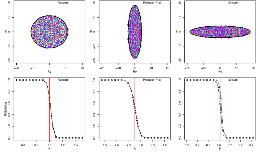
The value of can be derived for all the types of matrices illustrated above. In the random case, , and thus (i.e., the eigenvalues are distributed in a circle). For the predator-prey case, the expectation for the product is : the expectation for the product of two independent, identically distributed half-normal random variables, with a negative sign accounting for the opposite signs of the coefficients. Thus, , leading to , and . Similarly, for the mixture of competition and mutualism we have and thus .
These results hold for completely connected matrices, with ellipses centered at . Setting the diagonal coefficients to centers the ellipses at (for May’s results, ). For stable matrices, the ellipses must be fully contained in the left half-plane (), as the real part of all eigenvalues must be negative to attain stability. Accordingly, the stability criteria for fully connected matrices are: random, ; predator-prey, ; mixture of competition and mutualism, . To account for general connectance, , we follow May [1, 2] and include it under the square root, obtaining the stability criteria in Table 1.
| Interaction | Stability Criterion | |||
|---|---|---|---|---|
| Nested Mut. | 8 | 20 | 16 | |
| Mutualism | 8 (8.5) | 23 (24) | 18 (19.05) | |
| Bipartite Mut. | 9 | 24 | 19 | |
| Mixture | 11 (7) | 28 (23.9) | 41 (37.3) | |
| Competition | 12 | 33 | 50 | |
| Random | 26 (18.9) | 72 (64) | 109 (100) | |
| Niche Pred.-Prey | 75 | 202 | 295 | |
| Cascade Pred.-Prey | 125 | 417 | 649 | |
| Predator-Prey | 148 (143.4) | 482 (484.7) | 745 (757.3) | |
We have confirmed these results by plotting the density of the eigenvalues in the complex plane (Figure 1, top): even for matrices of moderate size (50 species or more), the approximation is very accurate. To show the sharpness of the transition from high to low probability of stability, we performed extensive numerical simulations (Figure 1, bottom).
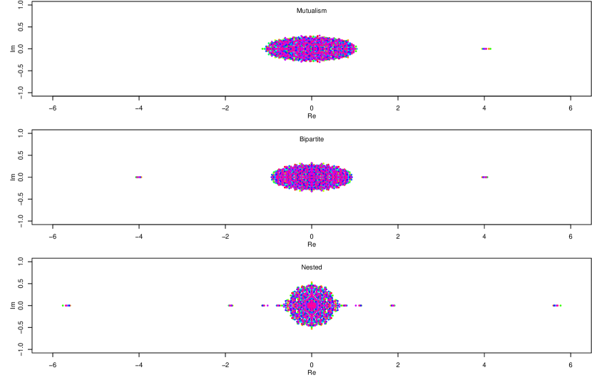
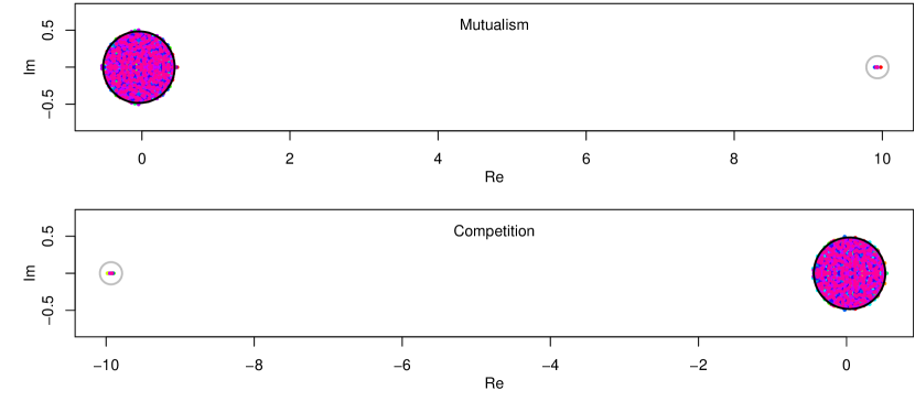
In all the above cases, , and the expected row (column) sum is also . What happens if we relax these constraints? The most extreme case is that of mutualism (, whereas are drawn from with probability and zero otherwise), in which the mean coefficient is and the expected row (column) sum is . In these matrices, we find an extreme, real eigenvalue , while the remaining eigenvalues (for ) are arranged in a circle centered at (Figure 2, top). Numerical simulations suggest that the radius of this circle is approximately . Because for mutualism the stability is determined exclusively by , the criterion becomes , which is equivalent to diagonal dominance [12]. Therefore, in this type of matrix the fact that interactions are arranged in pairs does not influence stability. For the competition case, the situation is reversed (Figure 2, bottom): we find an extreme negative eigenvalue , and the others are contained (for ), in a circle centered in with a radius of . The maximum eigenvalue is at the very right edge of the circle, so that we can derive a stability criterion only for : . For the general case in which , the non-extreme eigenvalues are approximately contained in an ellipse, but we have not found an exact expression for general .
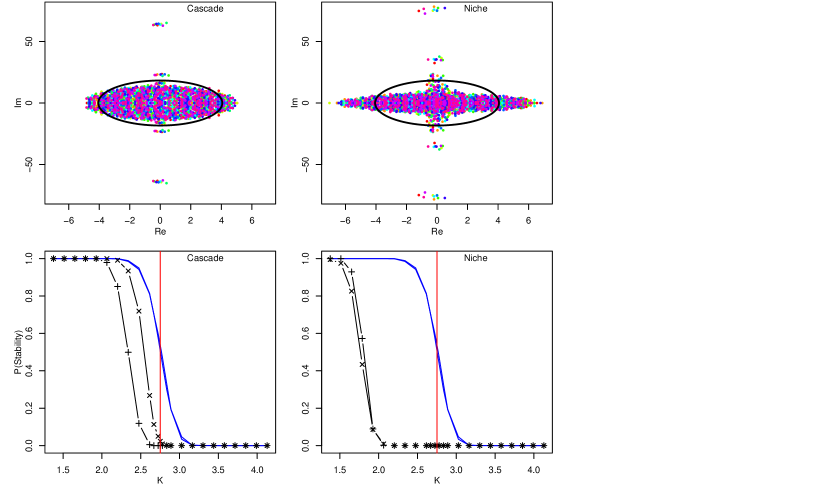
Returning to the predator-prey case, we assess the effect of imposing realistic food web structure. In community matrices describing food webs, we expect producers to have positive columns and negative rows, with the converse for top predators. These variations are likely to move some eigenvalues “vertically” in the complex plane (as the large row and column sums have opposite signs). To test this hypothesis, we plotted the eigenvalues for predator-prey webs in which interactions are arranged following the cascade [13] and niche [14] models (Appendix). Although these models cannot fully reproduce food web structure [14, 15, 16], they are widely used to simulate food webs (e.g., [17, 18]). It is generally believed that including realistic food web structure should increase stability (e.g., [19, 20]).
In both cases, we find several extreme eigenvalues with large imaginary part (Figure 3). Because the eigenvalues of these matrices must have the same mean and variance [10] observed in the unstructured predator-prey case, we observe a distortion of the ellipses, yielding larger real parts than expected. Thus, cascade and niche models should produce networks that are less stable than their unstructured predator-prey counterpart, with the niche model having a larger discrepancy. These considerations are confirmed by numerical experiments (Figure 3). We conclude that, surprisingly, imposing realistic food web structure hampers stability.
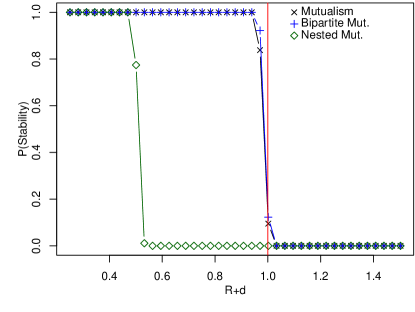
In the same spirit, we measured the effect realistic structures produce in mutualistic networks. Several published mutualistic networks are bipartite [21, 22, 23, 24]: there are two types of nodes (e.g., plants and pollinators), and interactions occur exclusively between different types. Also, bipartite mutualistic networks tend to be nested [21]: the interactions of the specialists are subset of those of the generalists. Nestedness is believed to beget stability [22, 23, 24]. We drew the eigenvalues for these two types of structure (bipartite, bipartite and nested Appendix, Figure 4), and contrasted the results with those obtained for the unstructured mutualistic case. We observed several large real eigenvalues as in the unstructured mutualistic case, but now for each positive eigenvalue we found an equally large negative one (Figure 4). The bipartite case yields row sums that are substantially similar to the unstructured case. Accordingly, we do not expect a large discrepancy in stability. However, given that nested structures will yield (on average), larger maximum row/column sum (associated with the generalist plants and animals), nested structures are inherently less stable than unstructured ones. These results are confirmed by numerical simulations (Figure 5).
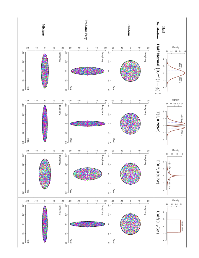
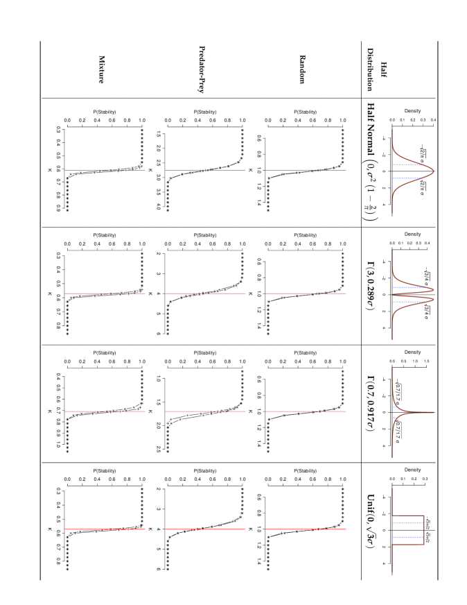
We have so far considered how the arrangement of the interaction coefficients affects stability, we now assess the role of interaction strength distributions. We have extracted coefficients from normal (or half-normal) distributions, where the majority of interactions are close to 0 and thus “weak”. These “weak interactions” are thought to contribute considerably to the stability and persistence of natural systems [25, 26]. To examine their effect, we extended our analysis to the cases in which the absolute value of each coefficient is taken either from a uniform or a gamma distribution, parametrized such that and (as in the normal case) (Appendix). Note that the different distributions represent different frequencies of weak interactions. Therefore, changing the distribution impacts , which, compared to the random case, has to be negative to increase stability and positive to depress stability. When weak interactions are preponderant, is expected to be smaller in magnitude. Therefore, weak interactions should increase the stability for mutualistic and competitive systems, but decrease the stability of predator-prey matrices and have no effect in the random case. This argument is matched by analytical and numerical results (Appendix), showing that, contrary to the current belief, weak interactions can be destabilizing.
To summarize the stability properties of the various matrices, we performed numerical simulations for all the types of networks and with three parametrizations (Table 1). We searched for the largest yielding a probability of stability (measured using 1000 matrices). In all cases, increases when moving from nested mutualism to predator-prey.
We have shown that arrangement into signed pairs of interactions has large impact on stability. For example, the random, mixture and predator-prey matrices contain basically the same coefficients, and the large difference in stability is driven exclusively by their arrangement (pairs with random signs, pairs with same sign and pairs with opposite signs, respectively). This is consistent with the fact that the variance of the eigenvalues is driven by the mean product between nonzero pairs .
Mutualism, competition, and their mixture, although yielding the same pairwise mean product, and the same mean and variance of the eigenvalues, have very different stability properties: increasing the fraction of competitive interactions increases stability. In these cases the stability is driven by higher moments of the eigenvalue distribution. We conjecture that the stability properties in these matrices are thus influenced by products of three or more coefficients at a time. For example, the product of three competitive interactions would yield a different sign from that of three mutualistic interactions, potentially accounting for the difference in stability.
Surprisingly, imposing realistic structure to the interaction networks appears to be detrimental for stability both in the predator-prey and the mutualistic cases. This does necessarily mean that more realistic networks should be less stable, as in our comparisons all the coefficients have (in absolute value) the same expectation, while this is not the case in natural systems (e.g., generalist species will have typically lower values for each interaction compared to specialists). However, we can safely assert that realistic structure alone is not contributing to stability: an increase in stability can be observed only if there is an interplay between the network structure and the interaction strengths. The fact that interaction strengths are a major determinant of stability is confirmed by our analysis showing that weak interactions can be either stabilizing or destabilizing depending on the type of interaction between species.
We have shown that simply plotting the density of the eigenvalues provides qualitative insight into the stability of the systems. Using this graphical method, the effect of any type of network structure can be readily analyzed.
Finally, we have found a consistent “stability hierarchy” spanning mutualism to predator-prey. Predator-prey interactions enable the stable coexistence of networks as large and complex as those observed empirically.
Our results are not limited to the stability of ecological (or biological) systems. The criteria, in fact, hold for any system of differential equations resting at an equilibrium point.
References
- [1] R.M. May, Nature 238, 413 (1972).
- [2] R.M. May, Stability and complexity in model ecosystems (Princeton Univ Pr, 2001).
- [3] S.L. Pimm, Nature 307, 321 (1984).
- [4] K.S. McCann, Nature 405, 228 (2000).
- [5] J.M. Montoya, S.L. Pimm, R.V. Solé, Nature 442, 259 (2006).
- [6] R. MacArthur, Ecology 36, 533 (1955).
- [7] C.S. Elton, Animal ecology (Univ Chicago Pr, 2001).
- [8] R. Levins, Evolution in changing environments: some theoretical explorations (Princeton Univ Pr, 1968).
- [9] S. Allesina, M. Pascual, Theor. Ecol. 1, 55 (2008).
- [10] J. Jorgensen, A.M.K. Rossignol, C.J. Puccia, R. Levins, P.A. Rossignol, Ecology 81, 2928 (2000).
- [11] H.J. Sommers, A. Crisanti, H. Sompolinsky, Y. Stein, Phys. Rev. Lett. 60, 1895 (1988).
- [12] R.S. Varga, Geršgorin and His Circles (Springer-Verlag, Berlin, 2004).
- [13] J.E. Cohen, F. Briand, C.M. Newman, Z.J. Palka, Community food webs: data and theory (Springer, 1990).
- [14] R.J. Williams, N.D. Martinez, Nature 404, 180 (2000).
- [15] M.F. Cattin, L.F. Bersier, C. Banašek-Richter, R. Baltensperger, J.P. Gabriel, Nature 427, 835 (2004).
- [16] S. Allesina, D. Alonso, M. Pascual, Science 320, 658 (2008).
- [17] X. Chen, J.E. Cohen, Proc. Roy. Soc. B 268, 869 (2001).
- [18] N.D. Martinez, R.J. Williams, J.A. Dunne, Ecological networks: linking structure to dynamics in food webs pp. 163–185 (2006).
- [19] S.J. McNaughton, Nature 274, 251 (1978).
- [20] P. Yodzis, Nature 289, 674 (1981).
- [21] J. Bascompte, P. Jordano, C.J. Melián, J.M. Olesen, Proc. Nat.l Acad. Sci. USA 100, 9383 (2003).
- [22] T. Okuyama, J.N. Holland, Ecol. lett. 11, 208 (2008).
- [23] U. Bastolla, et al., Nature 458, 1018 (2009).
- [24] E. Thébault, C. Fontaine, Science 329, 853 (2010).
- [25] K. McCann, A. Hastings, G.R. Huxel, Nature 395, 794 (1998).
- [26] M. Emmerson, J.M. Yearsley, Proc. Roy. Soc. B 271, 397 (2004).
- [27] Thanks to A. Eklof, R.M. May, P. Staniczenko for comments. Research supported by NSF EF # 0827493.
Appendix
Construction of the community matrices
In the main text we analyze different types of matrices. Here we detail how the matrices were constructed. In all cases, the parameters are: , number of species; , desired level of connectance; , standard deviation of the normal distribution from which coefficients are drawn; value of the diagonal coefficients. For each matrix, we also report the expected mean and variance for the eigenvalues.
Random Matrices
In the random case, we construct the matrices in the following way: i) for each coefficient , , we draw a random value from an uniform distribution . If the value is , we draw the coefficient from a normal . Otherwise (), . ii) All . For these matrices, the eigenvalues have and .
Predator-Prey Matrices
i) For each coefficient , , we draw a random value from . ii) If the value is , we draw a second random value from . If this new random value is , we draw from an half-normal distribution and from a negative half-normal , while if we do the opposite. iii) If , we assign to both coefficients. iv) All . For predator-prey, and .
Mixture of Competition and Mutualism Matrices
i) For each coefficient , , we draw a random value from . ii) If the value is , we draw a second random value from . If this new random value is , we draw and from an half-normal , while if we draw both coefficients from a negative half-normal distribution. iii) If , we assign to both coefficients. iv) All . For this mixture, and .
Mutualism Matrices
i) For each coefficient , , we draw a random value from . If the value is , we draw both and from an half-normal . Otherwise, we assign to both coefficients. ii) All . For mutualism, and .
Competition Matrices
i) For each coefficient , , we draw a random value from . If the value is , we draw both and from a negative half-normal . Otherwise, we assign to both coefficients. ii) All . For competition, and .
Cascade Predator-Prey Matrices
In the cascade model [13], species are ordered and each species has a fixed probability of preying upon the preceding species. The produced networks do not contain cycles, although cycles are observed in empirical networks [14]. In the cascade model, the species with highest ranking functions as a top predator, while that with the lowest ranking as a producer. Accordingly, the highest ranked has positive column and negative row, while the opposite is true for the lowest ranked.
The matrix construction algorithm is: i) For each coefficient , , we draw a random value from . If the value is , we draw the coefficient from an half-normal and the coefficient from a negative half-normal . Otherwise, we assign to both coefficients. ii) All . For the cascade model, and .
Niche Predator-Prey Matrices
The niche model [14] allows for trophic cycles and cannibalism. The species are ordered (each one being assigned a “niche value”, ). A “niche radius”, , proportional to , is drawn for each species along with a “niche center” . Each species preys upon all the species whose are included in the range . The produced networks are interval (i.e., each predator preys upon consecutive species). Empirical networks, however, are not perfectly interval [14, 15, 16].
To generate the matrices, we first produced an adjacency matrix , using the niche model ( if is a prey of ). Then we obtained a “sign matrix” . Finally, is obtained multiplying taken from an half-normal distribution by . The diagonal elements are set to . For the niche model, and .
Mutualistic Bipartite Matrices
For the bipartite case, we divided the species in two group of equal size (, when is even). For each where belongs to the first group and to the second, we draw and from an half-normal distribution with probability (so that the expected connectance is matched). The diagonal is . For the bipartite mutualistic model, and .
Mutualistic Nested Matrices
Nestedness is a property of the incidence matrix (typically rectangular) in which the row are the species belonging to the first group (e.g., plants) and the rows those in the second group (e.g., pollinators). Say that to match the desired connectance in the matrix , we want to arrange links in . We arrange the links in the following way: First, to guarantee connectedness, i) we fill the first row; ii) we fill the first column; iii) We arrange the subsequent links so that the matrix is perfectly nested. For example (using a squared incidence matrix), say that is :
and suppose we want to include 17 links. First, we fill the first row to , so that we placed 6 links. The next five links are used to fill the first column to . Finally, the last six links are placed in , , , , , etc. Note that the sum of the and coordinates for the links is growing. In fact, ordering the potential link by their coordinate sums, and giving precedence to those with smaller row number in case of ties, guarantees the maintenance of perfect nestedness. This is the filling algorithm we used in the simulations. Once we obtain , we use it (along with its transpose), to determine the interactions in the matrix . All the nonzero values of are taken from the half-normal . The diagonal is . For the bipartite nested mutualistic model, and .
Different Distributions and Weak Interactions
The goal of this section is to investigate whether our findings are robust to changes in the distribution of interaction strengths and to assess the role weak interactions play for stability. In the main text, we deal with normal (or half-normal) distributions. Here, we consider uniform distributions and gamma distributions with different shapes.
To measure how preponderant “weak interactions” are in a distribution of interaction strengths, we take the expectation for the absolute value. For example, for a normal distribution, define as a random variable taken from the distribution . The expectation for is (as we saw in the main text).
Before we can examine the other distributions, we have to parametrize them in such a way that and . In this way, we are satisfying the conditions we stated in the main text, and we are considering distributions of interaction strengths with the same mean and variance.
We start from a uniform distribution . We will sample positive coefficients from the distribution and negative coefficients reversing the sign. Thus, the interaction strengths (for the nonzero terms) are distributed uniformly in . Clearly, the distribution satisfies . When , the variance . With such a parametrization, the expected interaction is : typically, interactions will be larger than in the normal case. What are the consequences for stability? We begin by computing . For a predator-prey matrix whose elements are taken from the uniform distribution above, the expected product of the interaction strengths of two interacting species is and thus . This means that the stability criterion for uniform predator-prey becomes : the uniform predator-prey matrices are much more likely to be stable than their normal counterpart. The uniform random and mixture cases trivially follow. For the uniform random, : exactly as in the normal case. For the uniform mixture, , less than in the normal case. To summarize, for the uniform distribution (where we expect stronger interactions than in the normal case), we observe an increase in stability for the predator-prey case and a decrease for the mixture case. The random case in unaltered.
To further prove that weak interactions stabilize the mixture and destabilize the predator-prey cases, we analyzed the effect of taking the magnitude of the coefficients from a gamma distribution. The gamma distribution takes two parameters, (shape), and (scale). As above, we want to ensure that and . This is accomplished, for arbitrary , by choosing . For such a gamma distribution, . For example, for , (less than in the normal case), while for , (more than in the normal case, and exactly as in the uniform case). Computing for the predator-prey case, we find and thus the stability criterion becomes . This means a higher likelihood of stability, compared to the normal case, whenever (approximately, ). Thus, when we extract the magnitude of the coefficients from a gamma distribution, increasing will increase the expectation, and this in turn will result in more stability for the predator-prey case and less for the mixture (criterion: ). For the random case the situation is unaltered.
Our analytical predictions are confirmed by plotting the density of the eigenvalues (Figure 6) and drawing stability profiles (Figure 7) for all the distributions described above.
