Spin-orbit coupling induced enhancement of superconductivity in a two-dimensional repulsive gas of fermions

Abstract

We study a model of a two-dimensional repulsive Fermi gas with Rashba spin-orbit coupling $\alpha_{R}$, and investigate the superconducting instability using renormalization group approach. We find that in general superconductivity is enhanced as the dimensionless ratio $\frac{1}{2}m\alpha_{R}^{2}/E_{F}$ increases, resulting in unconventional superconducting states which break time reversal symmetry.

There is a growing interest in materials whose interfaces support a two-dimensional (2D) electron gas and display superconductivity, because of their novel, and potentially technologically useful properties such as electronic transport, magnetism and interplay between structural instabilitiesZubko et al. (2011); Ohtomo and Hwang (2004); Li et al. (2011). Due to the intrinsic breaking of the inversion symmetry, spin-orbit coupling is expected to play a role in determining the nature of the superconducting state. For example, experimentally the enhancement of transition temperature at LaAlO₃/SrTiO₃ interfaces tracks the enhancement of Rashba spin-orbit couplingCaviglia et al. (2010). And while the mechanism of superconductivity here is likely related to the electron-phonon mechanism of the bulk materialsKoonce et al. (1967), such considerations motivate us to investigate the effect of spin-orbit coupling on the superconducting transition.

For attractive interactions the question has been addressed in Ref.Edelshtein (1989); Gor’kov and Rashba (2001); Mineev and Sigrist (2009). In contrast, here we consider a model of repulsive fermions moving in 2D and analyze the nature of the unconventional superconducting state in weak coupling. For a strictly parabolic dispersion in 2D, without spin-orbit coupling, it is known that repulsive interactions do not induce superconductivity to second order in the interaction, unlike in 3D where $p$-wave superconductivity is found at this order. In 2D one has to go to third orderChubukov (1993) for the Kohn-Luttinger effects to appear. Our motivation is to understand the role of the spin-orbit coupling in this process, to determine whether it can enhance superconductivity, and to study the nature of the superconducting state. Since we treat the Rashba spin-orbit coupling $\alpha_{R}$ non-perturbatively, we can analyze the relative values of the mean-field transition temperatures $T_{c}$ for an arbitrary value of the dimensionless ratio $\Theta=\frac{1}{2}m\alpha^{2}_{R}/E_{F}$, where $m$ is the (bare) fermion mass and $E_{F}$ is the Fermi energy, measured from the Dirac point (see Fig. 1). In the strictest sense the transition in 2D is of Kosterlitz-Thouless type and at $T_{KT}<T_{c}$. However, since we are working in the weak coupling limit, the pairing energy scale is much smaller than the zero temperature phase stiffness energy and $1-T_{KT}/T_{c}\sim T_{c}/E_{F}(1+\Theta)\ll 1$, justifying the approach presented here.

Due to the spin-orbit interaction, the pair states cannot be chosen to be pure spin singlet or triplet, but appear as linear superposition thereofGor’kov and Rashba (2001). Nevertheless, since the Rashba model (2), as well as the short range repulsion (3), commute with the $z-$component of the total angular momentum $J_{z}=L_{z}+S_{z}$, we can label the pair states according to $\ell$, the eigenvalue of $J_{z}$. For small values of $\Theta$ we find that states with high values of relative angular momentum $\ell$ condense first, with $\ell$ decreasing as $\Theta$ increases. For intermediate values of $\Theta$ we find broad regions of stability for $\ell=4$, with dome-like dependence of $T_{c}$ on $\Theta$, while in the limit of large $\Theta$, we find $\ell=2$. In weak coupling we show that all of these states spontaneously break time-reversal symmetry. While we formulate our calculation within more modern renormalization group (RG) approach, our results can be rederived diagrammatically by summing the leading logarithms to all orders in perturbation theory, as has been done traditionally in treating Kohn-Luttinger effectGor’kov and Melik-Barkhudarov (1961); Baranov et al. (1992). Also, while our approach is similar to that of Ref.Raghu et al. (2010) (see alsoRaghu and Kivelson (2011)), we use a single step RG instead of a two step RG, which we find more economical.

Our starting point is the Hamiltonian for Fermions moving in 2D

$$\mathcal{H} = H_{kin}+H_{int}$$ (1)

where in momentum representation the kinetic energy (including spin-orbit coupling) is

$$H_{kin} = \sum_{{\bf k},\alpha\beta}c^{\dagger}_{{\bf k}\alpha}\left(\frac{{\bf k}^{2}}{2m}\delta_{\alpha\beta}+\alpha_{R}({\bm{\sigma}}_{\alpha\beta}\times{\bf k})\cdot\hat{{\bf n}}\right)c_{{\bf k}\beta}$$ (2)

and the short-range interaction energy term is

$$H_{int} = \frac{u}{2}\frac{1}{L^{2}}\!\!\!\!\!\sum_{{\bf k}_{1}\ldots{\bf k}_{4},\sigma\sigma^{\prime}}\!\!\!\!\!\delta_{{\bf k}_{1}+{\bf k}_{2},{\bf k}_{3}+{\bf k}_{4}}c^{\dagger}_{{\bf k}_{1}\sigma}c^{\dagger}_{{\bf k}_{2}\sigma^{\prime}}c_{{\bf k}_{3}\sigma^{\prime}}c_{{\bf k}_{4}\sigma}.$$ (3)

As usual, the components of ${\bf k}$ belong to the Born-von Karman set $\{2\pi n/L\}$ where $n$ is an integer and $L$ is the linear size of the system. Unlike in Ref.Gor’kov and Rashba (2001), we consider superconductivity for repulsive interactions, i.e. for $u>0$, in the weak coupling limit $u\nu_{2D}<<1$, where the density of states per spin in 2D for $\alpha_{R}=0$ is $\nu_{2D}=\frac{m}{2\pi}$. The kinetic energy term is diagonalized using the following transformation

$$\left(\begin{array}[]{c}c_{{\bf k}\uparrow}\\ c_{{\bf k}\downarrow}\end{array}\right)=\frac{1}{\sqrt{2}}\left(\begin{array}[]{cc}1&1\\ ie^{i\phi_{{\bf k}}}&-ie^{i\phi_{{\bf k}}}\end{array}\right)\left(\begin{array}[]{c}a_{{\bf k}+}\\ a_{{\bf k}-}\end{array}\right).$$ (10)

Next, we rewrite the Hamiltonian in terms of these helicity eigenmodes. The partition function associated with $\mathcal{H}$ can be expressed in terms of the coherent state Feynman path integral over Grassman variablesNegele and Orland (1998) as

$$Z=\int\mathcal{D}[a^{*}_{\lambda}(\tau)a_{\lambda}(\tau)]e^{-S_{0}-S_{int}}$$ (11)

where

$$S_{0} = \int_{0}^{\beta}d\tau\sum_{{\bf k},\lambda=\pm}a^{*}_{{\bf k}\lambda}(\tau)\left(\frac{\partial}{\partial\tau}+\epsilon_{{\bf k}\lambda}-\mu_{F}\right)a_{{\bf k}\lambda}(\tau),$$

$$S_{int} = \sum_{1,2,3,4}U(1,2,3,4)a^{*}(1)a^{*}(2)a(3)a(4),$$ (12)

where the single particle energies are (see Fig.1)

$$\epsilon_{{\bf k}\lambda}=\frac{{\bf k}^{2}}{2m}-\lambda\alpha_{R}k.$$ (13)

In the above expressions $\beta=1/(k_{B}T)$, $\mu_{F}$ is the exact chemical potential whose value depends on temperature $T$ and interaction $u$, in such a way as to preserve average particle density. We adopt a shorthand expression for the multiple summations $\sum_{1,2,3,4}(\ldots)\equiv\int_{0}^{\beta}d\tau_{1}\ldots d\tau_{4}\sum_{{\bf k}_{1}\ldots{\bf k}_{4}}\sum_{\mu\nu\lambda\rho}(\ldots)$,

$$U(1,2,3,4)=-\frac{u}{16L^{2}}\int_{0}^{\beta}d\tau\prod_{j=1}^{4}\delta(\tau-\tau_{j})\delta_{{\bf k}_{1}+{\bf k}_{2},{\bf k}_{3}+{\bf k}_{4}}$$

$$\times\left(\mu e^{-i\phi_{{\bf k}_{1}}}-\nu e^{-i\phi_{{\bf k}_{2}}}\right)\left(\lambda e^{i\phi_{{\bf k}_{3}}}-\rho e^{i\phi_{{\bf k}_{4}}}\right),$$ (14)

and $a(j)=a_{{\bf k}_{j}\alpha_{j}}(\tau_{j})$ where $\alpha_{j}=\{\mu,\nu,\lambda,\rho\}$ and $\phi_{{\bf k}}$ is an azimuthal angle in the momentum plane.

Figure 1: (Left) The dispersion relation. (Right) First order (tadpole) correction to self-energy.

We proceed by integrating out the high energy modes between the energy cutoff $A$ and $\Omega\ll A$ about the two Fermi surfaces at $T=0$. The expansion is organized by the powers of the dimensionless parameters $u\nu_{2D}$ and $\Omega/A$. At first order in the cumulant expansion, we find a correction to the chemical potential $\mu_{F}$ from the tadpole diagram shown in Fig.1. This correction is $\delta\mu_{F}=-\frac{1}{2}u(\langle\hat{\rho}_{+}\rangle+\langle\hat{\rho}_{-}\rangle)$, where $\hat{\rho}_{\pm}=\int\frac{d^{2}{\bf k}}{(2\pi)^{2}}a^{\dagger}_{{\bf k}\pm}a_{{\bf k}\pm}$. Such negative interaction correction must be absorbed in the chemical potential counterterm, $\mu_{F}-\mu^{(0)}_{F}=\frac{1}{2}u(\langle\hat{\rho}_{+}\rangle+\langle\hat{\rho}_{-}\rangle)+\mathcal{O}(u^{2})$, which is positive, and which guarantees that the average particle density remains fixed. In general, we are not aware of any argument why interactions should not renormalize the areas of the individual Fermi surfaces, while of course maintaining their sum fixed, but to first order we find no such renormalization.

Figure 2: (First row) 2^nd and 3^rd order corrections to the 4-pt scattering amplitude. (Second row) 4^th order correction. For the 3^rd and 4^th order terms, we display only the diagrams which contain logarithmic enhancement.

Superconducting instability comes from second and higher order terms in cumulant expansion. We first find the renormalization of the general four fermion term and then we place the pairs on the two Fermi surfaces, which are the only processes with logarithmic enhancements. To second order in $u$, and in the Cooper channel, we have the following correction to the effective interaction action $\delta S_{int}=$

$$\frac{u^{2}}{64L^{2}}\int_{0}^{\beta}\!\!d\tau\sum_{{\bf k}{\bf k}^{\prime}}\sum_{\mu\lambda}V_{\mu\lambda}({\bf k},{\bf k}^{\prime})a^{*}_{{\bf k}\mu}(\tau)a^{*}_{-{\bf k}\mu}(\tau)a_{-{\bf k}^{\prime}\lambda}(\tau)a_{{\bf k}^{\prime}\lambda}(\tau)$$

where the sum over ${\bf k},{\bf k}^{\prime}$ is restricted to a small window near the Fermi surfaces defined by indices $\mu$ and $\lambda$ within the energy $\Omega$ above and below $\mu_{F}$. We write

$$V_{\mu\lambda}({\bf k},{\bf k}^{\prime})=V^{pp}_{\mu\lambda}({\bf k},{\bf k}^{\prime})+V^{ph}_{\mu\lambda}({\bf k},{\bf k}^{\prime}),$$ (15)

where the two qualitatively different contributions, arising from the two 2^nd order diagrams shown in Fig.2 are

$$V^{pp}_{\mu\lambda}({\bf k},{\bf k}^{\prime}) = -8\mu\lambda(N_{+}+N_{-})e^{-i\phi_{{\bf k}}}e^{i\phi_{{\bf k}^{\prime}}}\ln\frac{A}{\Omega}$$ (16)

$$V^{ph}_{\mu\lambda}({\bf k},{\bf k}^{\prime}) = \Pi_{\mu\lambda}({\bf k},{\bf k}^{\prime})-\Pi_{\mu\lambda}(-{\bf k},{\bf k}^{\prime}).$$ (17)

The density of states on the two Fermi surfaces are $N_{\pm}=\nu_{2D}\left(1\pm\frac{\sqrt{\Theta}}{\sqrt{1+\Theta}}\right)$. In the second ”particle-hole” contribution

$$\Pi_{\mu\lambda}({\bf k},{\bf k}^{\prime})=\sum_{\alpha,\beta=\pm}\int\frac{d^{2}{\bf p}}{(2\pi)^{2}}\frac{n_{F}(\epsilon_{{\bf p}\alpha})-n_{F}(\epsilon_{{\bf p}+{\bf k}-{\bf k}^{\prime}\beta})}{\epsilon_{{\bf p}\alpha}-\epsilon_{{\bf p}+{\bf k}-{\bf k}^{\prime}\beta}}$$ (18)

$$\times \left(\mu e^{-i\phi_{-{\bf k}}}-\beta e^{-i\phi_{{\bf p}+{\bf k}-{\bf k}^{\prime}}}\right)\left(\lambda e^{i\phi_{-{\bf k}^{\prime}}}-\alpha e^{i\phi_{{\bf p}}}\right)$$

$$\times \left(\alpha e^{-i\phi_{{\bf p}}}-\mu e^{-i\phi_{{\bf k}}}\right)\left(\beta e^{i\phi_{{\bf p}+{\bf k}-{\bf k}^{\prime}}}-\lambda e^{i\phi_{{\bf k}^{\prime}}}\right),$$

where the Fermi occupation factor $n_{F}(x)=1/(e^{(x-\mu^{(0)}_{F})/T}+1)$, evaluated in the limit $T\rightarrow 0$. After a somewhat tedious, but otherwise straightforward analysis we find that we can write

$$\Pi_{\mu\lambda}({\bf k},{\bf k}^{\prime}) = 2me^{-i\phi_{{\bf k}}}e^{i\phi_{{\bf k}^{\prime}}}\Lambda_{\mu\lambda}(\Theta,\cos(\phi_{{\bf k}}-\phi_{{\bf k}^{\prime}}))$$ (19)

where $\Lambda_{\mu\lambda}(\Theta,\cos(\phi_{{\bf k}}-\phi_{{\bf k}}^{\prime}))$ is real. Note that under time reversal the helicity basis creation and annihilation operators transform as $\hat{K}a_{{\bf k}\pm}=\mp ie^{i\phi_{{\bf k}}}a_{-{\bf k}\pm}$ and $\hat{K}a^{\dagger}_{{\bf k}\pm}=\pm ie^{-i\phi_{{\bf k}}}a^{\dagger}_{-{\bf k}\pm}$ respectively, where we used $\phi_{-{\bf k}}=\phi_{{\bf k}}+\pi$. The above relation means that the Cooper channel potential $V_{\mu\lambda}({\bf k},{\bf k}^{\prime})$ pairs time reversed states, as it shouldMineev and Sigrist (2009). Inspecting the form of the remaining terms in (16) as well as the combination $\Lambda^{(S)}_{\mu\lambda}(\Theta,\cos\phi)=\frac{1}{2}\Lambda_{\mu\lambda}(\Theta,\cos\phi)+\frac{1}{2}\Lambda_{\mu\lambda}(\Theta,-\cos\phi)$ appearing in (17), shows that they are invariant under operations of the 2D rotation group. Additionally, since the remaining terms in the scattering amplitude are even under ${\bf k}\rightarrow-{\bf k}$, and independently under ${\bf k}^{\prime}\rightarrow-{\bf k}^{\prime}$, they can be decomposed into sum over even angular momentum channels

$$V^{ph}_{\mu\lambda}({\bf k},{\bf k}^{\prime})=4me^{-i\phi_{{\bf k}}}e^{i\phi_{{\bf k}^{\prime}}}\!\!\!\sum_{\ell=0,2,4,\ldots}\!\!\!V^{(\ell)}_{\mu\lambda}\cos(\ell(\phi_{{\bf k}}-\phi_{{\bf k}^{\prime}}))$$ (20)

where the dimensionless Fourier coefficients $V^{(\ell)}_{\mu\lambda}$ are functions of $\Theta$ and represent intra- and inter-band pairing amplitudes.

In order to determine $V^{(\ell)}_{\mu\lambda}$, we need to evaluate $\Lambda_{\mu\lambda}(\Theta,\cos\phi)$ in Eq.(19) from Eq.(18). We shift ${\bf p}\rightarrow{\bf p}-\frac{1}{2}{\bf Q}$ where ${\bf Q}={\bf k}-{\bf k}^{\prime}$, and transform from the polar coordinates to elliptical coordinates $x\in[1,\infty)$, $\psi\in[0,2\pi)$ by substituting $p_{\parallel}=\frac{1}{2}|{\bf Q}|x\cos\psi$ and $p_{\perp}=\frac{1}{2}|{\bf Q}|\sqrt{x^{2}-1}\sin\psi$. In the resulting expression $\psi$ appears only in $\cos\psi$, so we can substitute $y=\cos\psi$. For $\alpha=\beta$ we then perform the integral over $y$ first, which can be done in terms of elementary functions. Similarly, for $\alpha=-\beta$ we perform the integral over $x$ first. Our analysis is based on numerical integration of the remaining integral, which can be done quite fast to any desired accuracy. The final result for the antisymmetrized combination $\Lambda^{(S)}_{\mu\lambda}(\Theta,\cos\phi)$ is shown in the Fig.3.

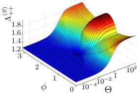
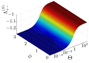
Figure 3: Relative angle $\phi=\phi_{{\bf k}}-\phi_{{\bf k}^{\prime}}$ and $\Theta=\frac{1}{2}m\alpha^{2}_{R}/E_{F}$ dependence of the interaction function $\Lambda^{(S)}_{\mu\nu}$ Eqs.(17-19) and text below. $\Lambda^{(S)}_{++}$ (top) and $\Lambda^{(S)}_{+-}$ (bottom) start from $\pm\frac{4}{\pi}$ at $\Theta=0$ and develop $\phi$ dependence for finite $\Theta$, while $\Lambda^{(S)}_{--}$ remains $\frac{4}{\pi}$ for any $\Theta$.

Next, we consider 3rd and 4th order terms in $u$ which renormalize the Cooper channel. These terms can be represented by diagrams shown in Fig 2, and used to derive the RG equations governing the flows of Cooper channel couplings, which decouple in the angular momentum basis. For $\ell\neq 0$ we find that the renormalized coupling

$${V^{r}}^{(\ell)}_{\mu\lambda}=\frac{u^{2}m}{2^{5}}V^{(\ell)}_{\mu\lambda}-\frac{u^{4}m^{2}}{2^{9}}\sum_{\alpha=\pm}N_{\alpha}V^{(\ell)}_{\mu\alpha}V^{(\ell)}_{\alpha\lambda}\ln\frac{A}{\Omega}+\ldots$$ (21)

where $\ldots$ represents term of order $u^{4}$ which do not contain (large) logarithm as well as terms of higher order in $u$. If we define a dimensionless coupling matrix $g^{(\ell)}_{\mu\lambda}=\frac{1}{2^{5}}u^{2}m\sqrt{N_{\mu}N_{\lambda}}V^{(\ell)}_{\mu\lambda}$ and take the logarithmic derivative of the right hand side in (21), then to, and including, $\mathcal{O}(u^{4})$, we find

$$\frac{d{g^{r}}^{(\ell)}_{\mu\lambda}}{d\ln\Omega} = 2\sum_{\alpha=\pm}{g^{r}}^{(\ell)}_{\mu\alpha}{g^{r}}^{(\ell)}_{\alpha\lambda}.$$ (22)

As usual, we have replaced the bare couplings by renormalized couplings to the order we are working. For $\ell\neq 0$, the initial condition for the above (matrix) differential equation is ${g^{r}}^{(\ell)}_{\mu\lambda}|_{\Omega=A}=\frac{1}{2^{5}}u^{2}m\sqrt{N_{\mu}N_{\lambda}}V^{(\ell)}_{\mu\lambda}$. This equation can be readily integrated by transforming into the orthonormalized basis for ${g^{r}}^{(\ell)}_{\mu\lambda}(\Omega)$ with eigenvalues

$${g^{r}}^{(\ell)}_{\pm}(\Omega)=\frac{{g}^{(\ell)}_{\pm}}{1+2{g}^{(\ell)}_{\pm}\ln\frac{A}{\Omega}}$$ (23)

where the initial eigenvalues of ${g^{r}}^{(\ell)}_{\mu\lambda}|_{\Omega=A}$, for $\ell\neq 0$, are

$${g}^{(\ell)}_{\pm} = \frac{u^{2}m}{2^{5}}\left(\frac{1}{2}(N_{+}V^{(\ell)}_{++}+N_{-}V^{(\ell)}_{--})\right.$$ (24)

$$\pm \left.\sqrt{\frac{1}{4}(N_{+}V^{(\ell)}_{++}-N_{-}V^{(\ell)}_{--})^{2}+N_{+}N_{-}{V^{(\ell)}}^{2}_{+-}}\right)$$

If ${g}^{(\ell)}_{\pm}<0$ for some $\ell$ or $\Theta$, then the associated renormalized coupling (23) diverges at a scale

$$T^{(\ell)}_{c}\sim{\Omega^{*}}^{(\ell)}=Ae^{-1/|g^{(\ell)}_{eff,\pm}|}$$ (25)

where $g^{(\ell)}_{eff,\pm}=2g^{(\ell)}_{\pm}$. While the assignment between $T_{c}$ and $\Omega^{*}$ cannot reliably determine the prefactor of the exponential term, the relative dependence on $\alpha_{R}$ is in the exponential factor, which we can determine. This allows us to compare the dependence of the ratio of (mean-field) transition temperatures on $\alpha_{R}$. For $\ell=0$ the equation $(\ref{eq:Vren ell neq0 RG})$ holds as well, provided that we modify the initial condition to ${g^{r}}^{(\ell=0)}_{\mu\lambda}|_{\Omega=A}=\frac{u}{4}\mu\lambda\sqrt{N_{\mu}N_{\lambda}}+\frac{1}{2^{5}}u^{2}m\sqrt{N_{\mu}N_{\lambda}}V^{(\ell=0)}_{\mu\lambda}$, and use the eigenvalues of this matrix in the Eq.(23).

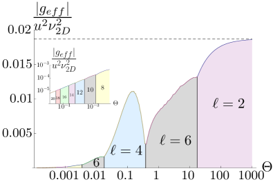
Figure 4: The effective coupling appearing in the expression for $T_{c}\approx Ae^{-1/|g_{eff}|}$ as a function of $\Theta=\frac{1}{2}m\alpha^{2}_{R}/E_{F}$. $\nu_{2D}=\frac{m}{2\pi}$. The dashed line at $0.0187$ is the $\Theta\rightarrow\infty$ asymptote.

To within our numerical accuracy, we find that $V^{(\ell=0)}_{--}=\frac{4}{\pi}$, while $V^{(\ell\neq 0)}_{--}=0$, for any $\Theta$. In addition, for $\Theta\gtrsim\mathcal{O}(0.01)$ most dominant angle dependence is in $V_{++}$, while there is only very weak angle dependence in $V_{+-}<0$. To $\mathcal{O}(u)$, $g^{(\ell=0)}_{+}>0$, meaning no pairing instability, and $g^{(\ell=0)}_{-}=0$. To $\mathcal{O}(u^{2})$ we find that $g^{(\ell=0)}_{-}>0$ for any $\Theta>0$, due to increase in both $V^{(\ell=0)}_{++}$ and $V^{(\ell=0)}_{+-}$, latter of which becomes less negative. This means that superconductivity resides predominantly on the large Fermi surface and is determined by some $V^{(\ell)}_{++}$ turning negative (meaning we select $-$ in Eq.(24)). In Fig.4 we show the $\Theta$ dependence of the couplings for the $g_{-}^{(\ell)}$-channel which has the highest $T_{c}$. At small value of $\Theta$, $\ell$ is very high (see inset of Fig.4). For the intermediate values of $\Theta$, starting with $\sim 0.005$, we find the sequence $\ell=6,4,6,2$, the last value of which continues to $\Theta\rightarrow\infty$.

Finally, we need to determine which linear combination of the two possible $\pm\ell$ states has the lowest (most negative) condensation energy as we go below $T_{c}$. Adopting the arguments of Anderson and MorelAnderson and Morel (1961), we study this problem below $T_{c}$ within mean-field. We replace the full angular dependence of the pairing potential with just its projection on the most dominant $\ell$ channel, an approximation which we expect to hold away from the boundaries separating ground states with different angular momentum. The self-consistent mean-field equations are then solved near $T_{c}$ and at $T=0$. We find either a solution which breaks time reversal symmetry and fully gaps the Fermi surface(s), i.e. only one of the two $\pm\ell$ pairing components is finite, or a solution with equal admixture of $\pm\ell$ and with gap nodes. Comparing their condensation energies we find that the time reversal breaking solution is lower by a factor of $1.5$ just below $T_{c}$ and by $e/2\approx 1.36$ at $T=0$. For values of $\Theta\gtrsim 0.005$, the gap on the larger Fermi surface is much larger than the gap on the smaller one due to the smallness of ratio of $V_{+-}/V_{++}$. For smaller value of $\Theta$ the two gaps may be comparable.

In summary, we have studied the superconducting instability of a 2D repulsive Fermi gas with Rashba spin-orbit coupling. We find that due to the polarizable fermion background, the repulsion turns into attraction on the large Fermi surface but not on the small one, giving rise to pairing there. Additional Josephson tunneling, $V^{(\ell)}_{+-}$, induces pairing on the small Fermi surface by (weak) proximity effect. The resulting unconventional superconducting states are found to break time reversal symmetry. While the transition temperature is not strictly monotonic in the dimensionless ratio $\Theta=\frac{1}{2}m\alpha_{R}^{2}/E_{F}$, the general trend is that it grows with increasing $\Theta$. This experimentally falsifiable feature, may provide means for enhancement of superconductivity in a larger class of 2D electron systems.

Acknowledgements: We wish to thank Prof. L. P. Gor’kov for useful discussions. This work is supported in part by NSF CAREER award under Grant No. DMR-0955561.

References

Zubko et al. (2011)
P. Zubko,
S. Gariglio,
M. Gabay,
P. Ghosez, and
J.-M. Triscone,
Annual Review of Condensed Matter Physics
2, 141 (2011).
Ohtomo and Hwang (2004)
A. Ohtomo and
H. Y. Hwang,
Nature 427,
423 (2004).
Li et al. (2011)
L. Li,
C. Richter,
J. Mannhart,
and R. C.
Ashoori, Nature Physics
7, 762 (2011).
Caviglia et al. (2010)
A. D. Caviglia,
M. Gabay,
S. Gariglio,
N. Reyren,
C. Cancellieri,
and J.-M.
Triscone, Phys. Rev. Lett.
104, 126803
(2010).
Koonce et al. (1967)
C. S. Koonce,
M. L. Cohen,
J. F. Schooley,
W. R. Hosler,
and E. R.
Pfeiffer, Phys. Rev.
163, 380 (1967).
Edelshtein (1989)
V. M. Edelshtein,
Sov. Phys. JETP 68,
1244 (1989).
Gor’kov and Rashba (2001)
L. P. Gor’kov and
E. I. Rashba,
Phys. Rev. Lett. 87,
037004 (2001).
Mineev and Sigrist (2009)
V. P. Mineev and
M. Sigrist,
ArXiv e-prints (2009),
eprint 0904.2962.
Chubukov (1993)
A. V. Chubukov,
Phys. Rev. B 48,
1097 (1993).
Gor’kov and
Melik-Barkhudarov (1961)
L. P. Gor’kov and
T. K. Melik-Barkhudarov,
Sov. Phys. JETP 13,
1018 (1961).
Baranov et al. (1992)
M. A. Baranov,
A. V. Chubukov,
and M. Y. Kagan,
International Journal of Modern Physics B
6, 2471 (1992).
Raghu et al. (2010)
S. Raghu,
S. A. Kivelson,
and D. J.
Scalapino, Phys. Rev. B
81, 224505
(2010).
Raghu and Kivelson (2011)
S. Raghu and
S. A. Kivelson,
Phys. Rev. B 83,
094518 (2011).
Negele and Orland (1998)
J. W. Negele and
H. Orland,
Quantum Many-particle Systems
(Westview Press, 1998), ISBN
0738200522.
Anderson and Morel (1961)
P. W. Anderson and
P. Morel,
Phys. Rev. 123,
1911 (1961).