Local density of states of two-dimensional electron systems under strong in-plane electric and perpendicular magnetic fields

Abstract

We calculate the local density of states of a two-dimensional electron system under strong crossed magnetic and electric fields. We assume a strong perpendicular magnetic field which, in the absence of in-plane electric fields and collision broadening effects, leads to Landau quantization and the well-known singular Landau density of states. Unidirectional in-plane electric fields lead to a broadening of the delta-function-singularities of the Landau density of states. This results in position-dependent peaks of finite height and width, which can be expressed in terms of the energy eigenfunctions. These peaks become wider with increasing strength of the electric field and may eventually overlap, which indicates the onset of inter-Landau-level scattering, if electron-impurity scattering is considered. We present analytical results for two simple models and discuss their possible relevance for the breakdown of the integer quantized Hall effect. In addition, we consider a more realistic model for an incompressible stripe separating two compressible regions, in which nearly perfect screening pins adjacent Landau levels to the electrochemical potential. We also discuss the effect of an imposed current on the local density of states in the stripe region.

I Introduction

The integer quantum Hall effect vKlitzing80:494 (IQHE) is one of the most important discoveries of condensed matter physics, observed on two-dimensional electron systems (2DES) subjected to a strong magnetic field $B$ perpendicular to the plane of the system. Measuring the low-temperature resistance in such systems, one finds that in certain $B$-intervals, the “plateau regimes” of the IQHE, the longitudinal resistance vanishes, indicating dissipationless transport, while the Hall resistance assumes quantized values, $R_{H}=h/(\nu e^{2})$, where $h=2\pi\hbar$ is Planck’s constant, $e$ the elementary charge, and $\nu$ a positive integer. An idealized homogeneous 2DES in a heterostructure (like GaAs/AlGaAs) without any scattering or interaction of the electrons, subjected to a homogeneous in-plane electric field, would yield the same resistance values. For this ideal 2DES, $\nu=2\pi\ell^{2}n_{\rm el}$ is the filling factor of the Landau levels, with energy eigenvalues $E_{n}=\hbar\omega_{c}(n+1/2)$ for $n=0,\,1,\dots$, $n_{\rm el}$ is the electron density, $\ell=\sqrt{c\hbar/e|B|}$ the magnetic length (we use CGS units, with $c$ the velocity of light), and $\omega_{c}=e|B|/(m^{*}c)$ the cyclotron frequency, with $m^{*}$ the effective mass ($m^{*}=0.067m_{e}$, for GaAs). In this paper we neglect spin-splitting of the Landau levels and take account of the spin degree of freedom by a degeneracy factor $g_{s}=2$. The fact, that in the IQHE one observes integer values of $\nu$, suggests that, in the plateau regime, the electrons which carry the current fully occupy an integer number of Landau levels, and thus are in states which are energetically separated from empty states, so that at low temperatures dissipative scattering processes are suppressed. Then one has to understand, why the relevant filling factor $\nu$ remains constant over a $B$-interval of finite width, and which processes limit the plateau regimes and lead back to dissipative transport.

If the effective filling factor has to be constant over an interval of $B$-values, obviously the relevant electron density must change. In the early attempts to explain this phenomenon, it has been assumed that the Coulomb interaction between the electrons is unimportant for the understanding of the IQHE. Localization theories PrangeGirvin ; Kramer03:172 stated that electron-impurity interaction leads to localized states in the tails of collision-broadened Landau levels, which do not contribute to the current transport. The existence of such inert localized states may explain the resistance quantization, even if a homogeneous current distribution is assumed. Such theories have, however, problems with explaining the enormous accuracy of better than $10^{-8}$, with which the quantized resistance values can be reproduced, Bachmair03:14 even in narrow Hall bars with a width of a few micrometers. Siddiki09:17007 The confinement of the 2DES to the interior of such Hall bars leads to edge states in the gaps between bulk Landau levels, which also have been considered to be important for the transport in the plateau regime of the IQHE. Halperin82:2185 ; Buettiker86:1761 This picture, which leads to extremely high current densities in the edge states and strongly $B$-dependent electron density profiles, has been critizised Chklovskii92:4026 because it neglects important screening effects.

The Landau quantization, which alters the energy-independent density of states (DOS) of the 2DES at $B=0$, $D_{0}=m^{*}/(\pi\hbar^{2})$, to the Landau DOS with sharp peaks around the Landau energies $E_{n}$, leads to peculiar screening effects, with nearly perfect screening if the Fermi energy $E_{F}$ (or the chemical potential) coincides with a Landau energy, and with no screening, if $E_{F}$ falls into a gap between two Landau levels.Efros88:1281 ; Efros88:1019 In an inhomogeneous 2DES, as e.g. in a Hall bar with electron depletion near the edges, this should lead to the occurrence of “compressible regions”, where a Landau level is pinned to the Fermi energy and the density is position-dependent, and “incompressible regions” which separate neighboring compressible regions with adjacent Landau levels at $E_{F}$. In these incompressible regions $E_{F}$ lies in the gap between two Landau levels, and one expects there a constant electron density corresponding to an integer value of the filling factor. Chklovskii92:4026 ; Chklovskii93:12605 ; Lier94:7757 ; Oh97:13519 Scanning force microscope experiments Weitz00:247 ; Ahlswede01:562 ; Ahlswede02:165 on narrow Hall bars have confirmed this picture. In the plateau regimes of the IQHE, the Hall potential across the sample drops across stripes at the positions predicted for incompressible stripes (ISs), and is constant elsewhere. Well outside the plateau regimes, the Hall potential varies nearly linearly between the sample edges. Self-consistent calculations for equilibrium Lier94:7757 ; Oh97:13519 and transport Guven03:115327 ; Siddiki04:195335 ; Gerhardts08:378 have clarified the situation. At sufficiently high temperature the conductivity is Drude-like, the current density $j_{y}(x)$ along the sample is proportional to the electron density $n_{\rm el}(x)$, and the Hall potential varies linearly across the sample. With decreasing temperature, near the lines of constant local filling factor $\nu(x)=2\pi\ell^{2}n_{\rm el}(x)=kg_{s}$ with even-inter values (since spin-degeneracy is assumed) local minima of the longitudinal resistivity develop (Shubnikov-deHaas effect), which lead to local maxima of the current density. With further decreasing temperature, ISs with extremely small values of the longitudinal resistivity develop along these lines and the current becomes confined to these stripes, where it can flow nearly without dissipation. It has been argued Siddiki04:195335 ; Gerhardts08:378 that an IS supporting dissipationless transport between two compressible regions can develop only if the distance between these regions is sufficiently large, larger than several times the extent of a typical wavefunction, say about $7\ell$, which requires a sufficiently slow variation of the effective potential. Siddiki10:113011 For the considered class of samples this guarantees that, in agreement with the experiments, the plateau regimes of the IQHE are well separated on the $B$-axis, and that only ISs with the same value of the local filling factor can exist simultaneously in the Hall bar.

If the stripe between two compressible regions becomes very small, one may expect that energy eigenfunctions with centers in different regions overlap and lead to quasi-elastic inter-Landau-level scattering (QUILLS), a mechanism which has been discussed for a long time as a possible reason for the breakdown of the IQHE under strong imposed currents. Eaves86:346 ; Guven02:155316 Such an overlap of wavefunctions, belonging to different Landau quantum numbers and having different center coordinates, but having the same energy eigenvalues, can occur in Landau levels tilted by a constant (Hall) electric field. A suitable quantity to study such overlap effects seems to be the local density of states (LDOS), which has recently been studied for such a constant-electric-field model and interpreted with respect to the IQHE, Kramer04:21 ; Kramer06:1243 however with a rather complicated mathematical approach and dubious results for the IQHE.

The purpose of this paper is to present a simple way to calculate the LDOS for a 2DES with translation symmetry in one in-plane direction, sect.II, to give explicit analytic and numeric results for simple model potentials in the other in-plane direction, sect.III, and, finally, to evaluate the LDOS for a simple but realistic model of an IS between two compressible regions, which carries an intrinsic and, possibly, an imposed external current, sect.IV.

II Electric-field-broadened Landau levels

We describe a 2DES in the $x$-$y$-plane, subjected to a strong magnetic field $\mathbf{B}=(0,0,B)=\nabla\times\mathbf{A(r)}$ in $z$-direction, in an effective-field (e.g. Hartree) approximation by a single-particle Hamiltonian

$$H=\frac{1}{2m^{*}}\Big{(}\mathbf{p}+\frac{e}{c}\mathbf{A(r)}\Big{)}^{2}+V(\mathbf{r}),$$ (1)

where the potential energy $V(\mathbf{r})$ may contain the effect of externally applied static electric fields, of lateral confinement, and of the average Coulomb interaction with the other electrons of the 2DES. Once the eigen-functions $\psi_{\alpha}(\mathbf{r})$ of the Schrödinger equation

$$(H-E_{\alpha})\psi_{\alpha}(\mathbf{r})=0$$ (2)

are known, one can calculate the electron density

$$n(\mathbf{r})=\sum_{\alpha}f_{\alpha}|\psi_{\alpha}(\mathbf{r})|^{2},$$ (3)

where the occupation probability $f_{\alpha}$ of the energy eigenstate $|\alpha\rangle$ may depend on all the quantum numbers of conserved quantities collected in $\alpha$, i.e., two for orbital motion and one for spin.

II.1 Local density of states (LDOS)

If in Eq. (3) the occupation probability of the state $|\alpha\rangle$ depends only on its energy eigenvalue, $f_{\alpha}=f(E_{\alpha})$, it may be useful to express the density

$$n(\mathbf{r})=\int dE\,f(E)\,D(E;\mathbf{r})$$ (4)

in terms of the “local density of states” (LDOS):

$$D(E;\mathbf{r})=\sum_{\alpha}\delta(E-E_{\alpha})|\psi_{\alpha}(\mathbf{r})|^{2}.$$ (5)

This formula for the LDOS is easily generalized to include the effect of quasi-elastic scattering of the electrons by randomly distributed impurities, which leads to a “collision broadening” of the $\delta$-function in Eq. (5). Systematic calculations of collision broadening Scher66:598 ; Keiter67:215 ; Bangert68:177 ; Gerhardts75:327 usually start from the Green operator $G_{\rm imp}(z)=(z-H-V_{\rm imp})^{-1}$ for a fixed impurity configuration, described by an impurity potential $V_{\rm imp}(\mathbf{r})$, and calculate approximately the average over all possible impurity configurations. This average is expressed in terms of a self-energy operator $\Sigma(z)$,

$$G(z)=[z-H-\Sigma(z)]^{-1}=\Big{\langle}G_{\rm imp}(z)\Big{\rangle}_{\rm imp}.$$ (6)

With $G^{+}(E)=G(E+i0^{+})$ the corresponding generalization of Eq. (5) reads

$$D(E;\mathbf{r})=-\frac{1}{\pi}{\rm Im}\langle\mathbf{r}|G^{+}(E)|\mathbf{r}\rangle.$$ (7)

Without impurities $\Sigma(z)\equiv 0$, and Eq. (7) reduces to Eq. (5), with the notation $\langle\mathbf{r}|\alpha\rangle=\psi_{\alpha}(\mathbf{r})$.

II.2 Translation symmetry in $y$-direction

In the following we assume that the system is translation-invariant in $y$-direction, but electric fields in $x$-direction, $\mathbf{E}=(E_{x},0,0)=\nabla V(x)/e$, will be allowed. The translation invariance in $y$-direction suggests the Landau gauge $\textbf{A}(\textbf{r})=(0,xB,0)$ for the vector potential, so that the single-electron Hamiltonian (1) becomes cyclic in $y$ and allows the separation ansatz

$$\psi(x,y)=\frac{e^{iky}}{\sqrt{L_{y}}}\,\varphi_{k}(x),$$ (8)

where $L_{y}$ ($\rightarrow\infty$) is the normalization length in $y$ direction, and the quasi-continuous momentum quantum number $k$ assumes the values $k=2\pi n_{y}/L_{y}$, for arbitrary integers $n_{y}$. With this ansatz the Schrödinger equation (2) reduces to the one-dimensional form

$$H_{X}\varphi_{n,X}(x)=E_{n}(X)\varphi_{n,X}(x),$$ (9)

with the effective Hamiltonian

$$H_{X}=-\frac{\hbar^{2}}{2m^{*}}\frac{d^{2}}{dx^{2}}+\frac{m^{*}}{2}\omega_{c}^{2}(x-X)^{2}+V(x),$$ (10)

where $X=-\ell^{2}k$ denotes the center of the parabolic potential, which describes the effect of the magnetic field and leads for fixed $X$ to a discrete energy spectrum $E_{n}(X)$. Here and in the following we neglect spin splitting and consider spin by a degeneracy factor $g_{s}=2$. In general the eigenstates $\langle\mathbf{r}|n,X\rangle$ carry current in $y$-direction, and the expectation value of the velocity operator $\hat{v}_{y}$ is given by (Hellmann-Feynman theorem)

$$\langle n,X|\hat{v}_{y}|n,X\rangle=-\frac{1}{m^{*}\omega_{c}}\frac{dE_{n}(X)}{dX}\quad\Big{[}\equiv\frac{1}{\hbar}\frac{dE_{n}}{dk}\Big{]}.$$ (11)

Then the electron density, Eq. (3), depends only on $x$,

$$n(x)=\frac{g_{s}}{2\pi\ell^{2}}\sum_{n}\int dX\,f_{n,X}\,|\varphi_{n,X}(x)|^{2},$$ (12)

and is accompanied by a current density

$$j_{y}(x)=\frac{g_{s}e}{2\pi\hbar}\sum_{n}\int dX\,f_{n,X}\,\frac{dE_{n}(X)}{dX}|\varphi_{n,X}(x)|^{2}.$$ (13)

The LDOS, Eq. (5), reduces to

$$D(E;x)\!=\!\frac{g_{s}}{2\pi\ell^{2}}\sum_{n}\!\int\!dX\delta(E\!-\!E_{n}(X))\,|\varphi_{n,X}(x)|^{2}.$$ (14)

If the dependence of $E_{n}(X)$ on $X$ is smooth enough to allow for a Taylor expansion around the center coordinate $X_{n,E}$ defined by $E_{n}(X_{n,E})=E$, the $X$-integral in Eq. (14) can be evaluated:

$$D(E;x)=\frac{g_{s}}{2\pi\ell^{2}}\sum_{n}\frac{|\varphi_{n,X_{n,E}}(x)|^{2}}{|E^{\prime}_{n}(X_{n,E})|},$$ (15)

with $E^{\prime}_{n}(X_{n,E})=dE_{n}/dX(X_{n,E})$. Before we illustrate some properties of this LDOS with typical examples, we introduce a simple treatment of collision broadening.

II.3 Collision broadening

II.3.1 Homogeneous 2DES without electric field

For $V(x)\equiv 0$ we get the well known Landau problem with energy eigenvalues and eigenfunctions

$$E_{n}=\hbar\omega_{c}(n+\frac{1}{2}),\quad\varphi_{n,X}(x)=\frac{1}{\sqrt{\ell}}\,u_{n}\Big{(}\frac{x-X}{\ell}\Big{)},$$ (16)

respectively, where the normalized oscillator wavefunctions,

$$u_{n}(\zeta)=\Big{(}\frac{1}{2^{n}n!\sqrt{\pi}}\Big{)}^{1/2}\,H_{n}(\zeta)\,e^{-\zeta^{2}/2},$$ (17)

are given by the Hermite polynomials $H_{n}(\zeta)$ of order $n$.Abramowitz Since here the energy eigenvalues are independent of $X$, the $X$-integral in Eq. (14) reduces to the normalization integral of the eigenfunctions, and the LDOS reduces to the well known Landau DOS of the homogeneous system

$$D(E;x)=\frac{g_{s}}{2\pi\ell^{2}}\sum_{n}\delta(E-E_{n}),$$ (18)

which does not depend on the position $x$. To include the effect of collision broadening, one has to evaluate the self-energy operator. With weak assumptions (like rotation symmetry) on the impurity potentials, one can show that $\Sigma(z)$ and the Green operator $G(z)$ are diagonal in the Landau representation, and that the matrix elements together with the eigen-energies $E_{n}(X)$ do not depend on $X$. Scher66:598 ; Keiter67:215 ; Bangert68:177 ; Gerhardts75:327 Then in Eq. (18) the singular $\delta(E-E_{n})$ is replaced by a spectral function $A_{n}(E-E_{n})$ of finite width. Depending on the approximation scheme, several analytical forms for the spectral function have been obtained. The self-consistent Born approximation (SCBA)Gerhardts75:327 ; Ando82:437 leads, if scattering between different Landau levels is neglegted, to a semi-elliptical form,

$$A_{n}^{\rm SCBA}(E-E_{n})=\frac{1}{\pi\Gamma_{n}}\Big{(}1-\Big{[}\frac{E-E_{n}}{2\Gamma_{n}}\Big{]}^{2}\Big{)}^{\frac{1}{2}},\,$$ (19)

while other approaches yield a Gaussian form, Gerhardts75:285

$$A_{n}^{G}(E-E_{n})=\frac{1}{\sqrt{2\pi}\,\Gamma_{n}}\exp\Big{(}-\frac{1}{2}\Big{[}\frac{E-E_{n}}{\Gamma_{n}}\Big{]}^{2}\Big{)}.$$ (20)

In the limit of short-range impurity potentials the matrix elements of the self-energy and thereby the $\Gamma_{n}$ in Eqs. (19) and (20) become even independent of the Landau quantum number $n$.

II.3.2 Model for non-homogeneous systems

We now consider the more general case that the effective Hamiltonian (10) contains a position-dependent potential $V(x)$. For each value $X$ of the center coordinate this leads again to a discrete energy spectrum, but these generalized Landau energies usually depend on $X$ and form dispersive Landau bands with energies $E_{n}(X)$.

As mentioned above, in the absence of electric fields the Landau energy eigenvalues do not depend on the center coordinate $X$, and as a consequence Green and self-energy operator are diagonal in the Landau representation and independent of $X$. In the presence of electric fields, however, the eigen-energies depend on $X$, and so do Green and self-energy operators. Moreover we can show that both are no longer diagonal in the generalized Landau representation, which diagonalizes the Hamiltonian in the absence of collisions. This more complicated situation is found even in the case of short-range impurity potentials, which for homogeneous systems with $V(x)\equiv 0$ leads to the same collision broadening for all Landau levels. Then the evaluation of collision broadening effects becomes much more complicated, and exceeds the scope of the present paper.

For weak electric field $E_{x}$, on the other hand, the formula

$$D(E;x)\!=\!\frac{g_{s}}{2\pi\ell^{2}}\!\!\sum_{n}\!\!\int\!\!dX\,A_{n}\big{(}E\!-\!E_{n}(X)\big{)}\,\varphi_{n,X}^{2}(x),\,~{}$$ (21)

which is correct for $E_{x}=0$ and a straighforward generalization of Eq. (5), should yield a reasonable description of collision broadening effects. Since we are not aware of a better, practicable approach to treat collision broadening in the presence of electric fields, we will in the following use Eq. (21) as a phenomenological rule to estimate the consequences of such scattering effects.

III Exactly solvable models

III.1 Constant electric field

Simple analytic results are also obtained for the case of a constant in-plane electric field $\mathbf{E}=(E_{x},0,0)$, leading to the potential $V(x)=exE_{x}$. Within classical mechanics, this leads for an ideal 2DES to a constant Hall drift of the centers of the cyclotron motion, which can be eliminated by a Galilei transformation to a coordinate system moving with the drift velocity $\mathbf{v}_{D}=c\mathbf{E\times B}/B^{2}=(0,-cE_{x}/B,0)$. Since all electrons suffer the same drift velocity, the current density $\mathbf{j}(x)=-e\mathbf{v}_{D}n(x)$ is proportional to the electron density $n(x)$, and one obtains Ohm’s law $\mathbf{j}(x)=\hat{\sigma}(x)\mathbf{E}$ with the Hall conductivity $\sigma_{yx}(x)=(ec/B)n(x)$ and vanishing longitudinal conductivity, $\sigma_{xx}(x)\equiv 0$.

III.1.1 Eigenstates and LDOS

Inserting $V(x)=exE_{x}$ into the Hamiltonian (10) results in a shifted parabolic potential with the new center $\tilde{X}=X-eE_{x}/(m^{*}\omega_{c}^{2})$ and position-independent terms, which add to the oscillator energies $\varepsilon_{n}=\hbar\omega_{c}(n+1/2)$. The resulting energy eigenvalues and eigenfunctions are

$$\tilde{E}_{n}(\tilde{X}) = \varepsilon_{n}+eE_{x}\tilde{X}+\frac{m^{*}}{2}v_{D}^{2}$$ (22)

$$= \varepsilon_{n}+eE_{x}X-\frac{m^{*}}{2}v_{D}^{2}\equiv E_{n}(X),$$

and

$$\varphi_{n,X}(x)=\frac{1}{\sqrt{\ell}}\,u_{n}\Big{(}\frac{x-\tilde{X}}{\ell}\Big{)},$$ (23)

respectively, with $v_{D}=cE_{x}/B$. From Eq. (11) we see that each state carries the same current $-e\langle n,X|\hat{v}_{y}|n,X\rangle=e^{2}E_{x}/m^{*}\omega_{c}=ev_{D}$, in analogy to the fact, that the radius of the classical cyclotron orbit has no influence on the drift velocity of its center. As a consequence of Eqs. (12) and (13) the current density is directly proportional to the electron density,

$$j_{y}(x)=ev_{D}n(x),$$ (24)

independent of the occupation probability of the eigenstates, just as in the classical case.

Due to the linear dependence of $\tilde{E}_{n}(\tilde{X})$ on $\tilde{X}$, Eq. (15) can be written as

$$D(E;x)=\frac{g_{s}}{2\pi\ell^{2}}\sum_{n}\frac{1}{e|E_{x}|\ell}\,u_{n}^{2}\Big{(}\frac{\tilde{E}_{n}(x)-E}{eE_{x}\ell}\Big{)}.$$ (25)

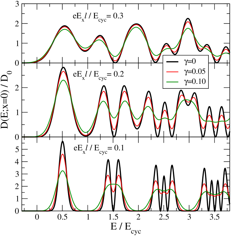
Figure 1: (color online) Heavy black lines ($\gamma=0$): LDOS according to Eq. (25) for three values of the electric field strength, $|eE_{x}|\ell/\hbar\omega_{c}=0.1,\,0.2$ and $0.3$. Also shown is the effect of level broadening according to Eqs. (21) and (20) for $\gamma\equiv\Gamma/\hbar\omega_{c}=0.05$ and $0.1$. $D_{0}=m^{*}/(\pi\hbar^{2})$, $g_{s}=2$.

This result has been obtained in Ref. [Kramer04:21, ] in a much less transparent way, starting from the symmetric instead of the Landau gauge for the vector potential.

Since in Eq. (25) the argument of the wavefunctions depends linearly on both, the position $x$ and the energy $E$, the energy dependence of the LDOS reflects the position dependence of the energy eigenfunctions. The contributions of the individual Landau levels, which become $\delta$-function like for vanishing $E_{x}$, become wider with increasing electric field, with a width proportional to $eE_{x}\ell$. If one shifts the position from $x$ to $x+a$, one obtains the same profile for the LDOS, but shifted on the energy axes by $-eE_{x}a$: $D(E;x+a)=D(E-eE_{x}a;x)$. Typical results Kramer04:21 for the LDOS according to Eq. (25) are shown by the heavy black lines in Fig. 1. It is seen that the gaps between the lowest adjacent Landau levels close for $0.1<eE_{x}\ell/\hbar\omega_{c}<0.2$, whereas the zeroes of the LDOS determined by the zeroes of the eigenfunctions remain rather stable.

If contributions to the LDOS due to adjacent Landau levels overlap, this means that, at the same position and at the same energy wavefunctions due to different Landau levels have finite values. Then, if there is also a non-vanishing impurity potential at this position, the potential matrix element between these adjacent levels is finite and there must be elastic scattering between these levels. This quasi-elastic inter-Landau-level scattering (QUILLS) has been discussed for a long time Eaves86:346 ; Guven02:155316 as a possible mechanism for the breakdown of the IQHE under strong imposed currents. Apparently QUILLS must become important in the neighborhood of narrow incompressible strips, where the local potential must bridge an amount of order $\hbar\omega_{c}$ across a strip of a width less than about $10\ell$.

The colored lines in Fig. 1 are calculated from Eq. (21) for a Gaussian spectral function, Eq. (20), with $n$-independent $\Gamma_{n}=\gamma\,\hbar\omega_{c}$ for two values of $\gamma$. Apparently the zeroes of the LDOS, which are due to the zeroes of the energy eigenfunctions, are smeared out already by a very weak collision broadening, and are of no importance in real samples. A discussion Kramer04:21 of a possible importance of these zeroes for the QHE is therefore without any relevance. On the other hand, the value of the LDOS in the gap between two adjacent Landau levels is of importance. In order to yield a plateau in the IQHE, the gap in an incompressible strip between two adjacent compressible regions must be sufficiently well developed. As a measure for the quality of such gaps we may consider the overlap of the contributions of adjacent Landau levels to the LDOS, according to Eq. (25). We define the overlap as the product of these contributions in the middle $E_{n,n+1}(x)=[\tilde{E}_{n}(x)+\tilde{E}_{n+1}(x)]/2$ between these levels, devided by the square of the zero-$B$ DOS $D_{0}=m^{*}/(\pi\hbar^{2})$, to make the overlap dimensionless. Since $g_{s}/(2\pi\ell^{2}D_{0})=\hbar\omega_{c}$, Eqs. (22) and (25) yield for the dimensionless overlap of level $n$ and $n+1$:

$$O_{n,n+1}(\eta)=\frac{1}{\eta^{2}}\,u_{n}^{2}\big{(}-\frac{1}{2\eta}\big{)}\,u^{2}_{n+1}\big{(}\frac{1}{2\eta}\big{)},$$ (26)

with $\eta=e|E_{x}|\ell/\hbar\omega_{c}$. The results for the lowest gaps, $O_{0,1}(\eta)=\exp(-1/2\eta^{2})/(2\pi\eta^{4})$ and $O_{1,2}(\eta)=O_{0,1}(\eta)(2-1/\eta^{2})^{2}/8$, are plotted in Fig. 2.

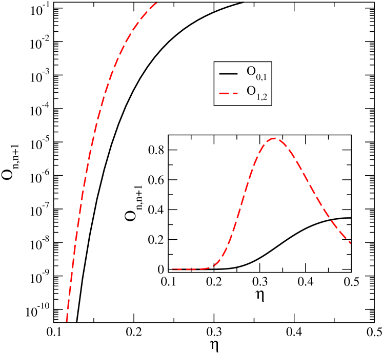
Figure 2: Dimensionless overlap for the two lowest Landau gaps as function of $\eta=e|E_{x}|\ell/\hbar\omega_{c}$.

If we say that the gap between Landau level $n$ and $n+1$ is well developed if $O_{n,n+1}<10^{-8}$, this defines a critical value $\eta_{n,n+1}^{cr}$ ($\eta_{0,1}^{cr}\approx 0.15$, $\eta_{1,2}^{cr}\approx 0.13$) and thereby a critical field-strength $E_{n,n+1}^{cr}=\eta_{n,n+1}^{cr}\hbar\omega_{c}/e\ell$. Only for sufficiently small electric fields with

$$|E_{x}|\lesssim 2.1\eta_{n,n+1}^{cr}(B/10{\rm T})^{3/2}\times 10^{6}\,{\rm V/m}$$ (27)

the gap between the Landau levels $n$ and $n+1$ is well developed. An equivalent formula, with $2.1\eta_{n,n+1}^{cr}$ replaced by $1/[\sqrt{2n+1}+\sqrt{2n+3}]$, was given in Eq. (41) of Ref. Kramer04:21, as experimentally verified criterion for the breakdown of the IQHE.

III.1.2 Occupation of eigenstates

The properties of a 2DES are not only determined by the properties of the single-particle eigenstates, but also by their occupation. Here we consider two different examples.

According to the general rules of statistical mechanics, a thermal equilibrium state is characterized by the expectation values of its conserved quantities, which in our case are (1) the particle number, or for fixed volume the average particle density, (2) the energy, and (3) the quasi-momentum in $y$-direction, $\hat{p}_{y}$ with eigenvalues $\hbar k=-m^{*}\omega_{c}X$, related to the translation symmetry. The grand canonical distribution function under these boundary conditions yields

$$f_{n,X}=f(\beta[E_{n}(X)-\mu-\hbar v_{y}X/\ell^{2}]),$$ (28)

with $f(x)=1/(1+e^{x})$ the Fermi-Dirac function and $\beta=1/k_{B}T$, $-\beta\mu$, and $-\beta\hbar v_{y}/\ell^{2}$ Lagrange multipliers conjugated to the conserved quantities energy, particle number, and quasi-momentum, respectively.

Constant electron density.

If we choose $v_{y}=v_{D}$, equal to the classical Hall drift velocity, the argument of the distribution function becomes independent of $X$, and the $X$-integral in Eq. (12) reduces to the normalization integral of the wavefunctions, so that the electron density becomes independent of the position $x$ and is given by

$$n(x)\equiv\bar{n}_{\rm el}=\frac{g_{s}}{2\pi\ell^{2}}\sum_{n}f(\beta[\varepsilon_{n}-m^{*}v_{D}^{2}/2-\mu]),$$ (29)

which apart from an unimportant shift of the energy zero is the same as in the absence of the electric field $E_{x}$. This choice of the Lagrangian multiplier apparently describes the quantum analog of the homogeneous Hall system, with spatially constant electron and current densities.

Considered as a function of the chemical potential, the electron density $\bar{n}_{\rm el}(\mu)$ for fixed magnetic field is a step-function, with steps of height $g_{s}/(2\pi\ell^{2})$ and a width of the order of $k_{B}T$ (or of $\Gamma_{n}$ if collision broadening is considered), located near the Landau energies $\mu\approx\varepsilon_{n}$. At low temperatures, $k_{B}T\ll\hbar\omega_{c}$, (and for weak collision broadening, $\Gamma_{n}\ll\hbar\omega_{c}$) these steps are separated by wide plateaus of constant $\bar{n}_{\rm el}(\mu)$, where $\mu$ varies in the gap between two adjacent Landau levels (LLs). In these plateaus there are no states at the Fermi energy (i.e. near $\mu$) and no quasi-elastic scattering is possible. Therefore, the longitudinal conductivity is zero and the Hall conductivity has the quantized value $\sigma_{H}=e^{2}\nu/h$ with an integer value of the filling factor $\nu=2\pi\ell^{2}\bar{n}_{\rm el}(\mu)$, even if one allows for quasi-elastic impurity scattering, which may lead to dissipation if $\mu$ is located in a broadened LL. This scenario is considered in Ref. [Kramer04:21, ] in order to explain the IQHE. The same physical situation can be considered for constant $\mu$ and varying magnetic field $B$. With increasing $B$ both the degeneracy $g_{s}/(2\pi\ell^{2})$ of the LLs and their energies $\varepsilon_{n}$ increase linearly with $B$. If $\mu$ is within a temperature and collision broadened LL, we may observe dissipation and the conductivity components are not quantized. With increasing $B$ the energy of this broadened level rises above the chemical potential, which then falls into the gap below this broadened level. Then the electron density increases at constant filling factor linearly with $B$, and the conductivity components are quantized, until the next lower broadened LL reaches the energy $\mu$. The dissipation sets in again, and the filling factor decreases by $g_{s}$ as this level passes the fixed chemical potential, which causes a rapid decrease of the electron density.

If in the low-temperature transport experiments on 2DESs the chemical potential would be constant, this scenario would explain the IQHE. This scenario, which at low filling factors requires that changing the magnetic field induces large density changes (up to 50%), is, however, unrealistic. In real experiments such a large electron exchange between the 2DES and its surrounding is hardly possible, and the assumption of constant electron density is much more realistic than that of constant chemical potential. For constant $\bar{n}_{\rm el}(\mu)$, Eq. (29) requires that $\mu$ oscillates as a function of $B$, and these oscillations have indeed been observed experimentally. Wei97:2514 ; Wei98:496 If a broadened LL is completely occupied, a further lowering of $B$ at constant $\bar{n}_{\rm el}(\mu)$ requires, that $\mu$ jumps to the lower edge of the next higher LL, so that the quantized values of the conductivity components occur only at a single, isolated value of $B$, not in a whole $B$-interval. This explains the well-known Shubnikov-deHaas effect, but not the IQHE as is claimed in Ref. [Kramer04:21, ]. The attempts of Refs. [Kramer04:21, ] and [Kramer06:1243, ] to calculate the conductivity tensor are also not compatible with accepted transport theories Gerhardts75:327 ; Ando82:437 and yield incorrect results.

If one writes in Eq. (28) $\mu^{*}(X)=\mu-\hbar v_{y}X/\ell^{2}$ and replaces the center coordinate by the position $x$, one gets a position-dependent electrochemical potential $\mu^{*}(x)$. This may reasonably describe a stationary non-equilibrium, and possibly dissipative, state as is found in a quantum Hall system outside the plateau regime of the QHE.Guven03:115327 ; Siddiki04:195335 In a thermal equilibrium state, however, the electrochemical potential $\mu^{*}$ must be spatially constant and can depend only on eigenvalues of conserved quantities, such as $X$ and $E_{n}(X)$.

A 2DES with homogeneous electron and Hall current densities may be a good approximation to the interior of a laterally confined system, far away from the edges. The same single particle states and energies may, however, also be used to describe an edge region of a laterally confined system.

Variable electron density.

Let us now focus on an edge region and assume that the confinement potential there can be approximated by the linear potential $V(x)=eE_{x}x$. Let us further assume that the total, laterally confined, system is in thermodynamic equilibrium, with vanishing total current. To describe such a state, we put in Eq. (28) $v_{y}=0$ and take a fixed constant value $\mu^{*}$ for the electrochemical potential.

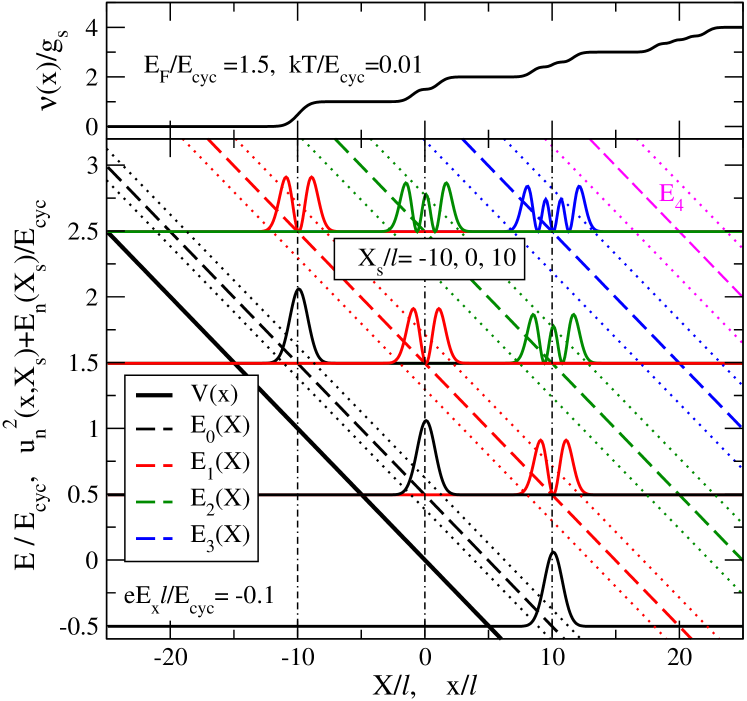
Figure 3: (color online) Upper part: filling factor $\nu(x)=2\pi\ell^{2}n(x)$ for $\mu^{*}=1.5\hbar\omega_{c}$, $k_{B}T=0.01\hbar\omega_{c}$; lower part: potential $V(x)=eE_{x}x$, energies $E_{n}(X)$ (dashed lines) and the wavefunctions squared at $X_{s}=0$ and $X_{s}=\pm\hbar\omega_{c}/eE_{x}$, shifted by their eigenenergies in units of the cyclotron energy $E_{\rm cyc}=\hbar\omega_{c}$. In both parts $\eta=eE_{x}\ell/\hbar\omega_{=}-0.1$. The dotted lines indicate the spatial extent of the wavefunctions.

Then the electron density can be calculated directly from Eq. (12) or, equivalently, from the LDOS (25),

$$n(x) = \frac{g_{s}}{2\pi\ell^{2}}\sum_{n}\int\frac{d\tilde{X}}{\ell}f\Big{(}\frac{\tilde{E}_{n}(\tilde{X})-\mu^{*}}{k_{B}T}\Big{)}\,u_{n}^{2}\Big{(}\frac{x-\tilde{X}}{\ell}\Big{)}$$ (30)

$$= \int dE\,f\Big{(}\frac{E-\mu^{*}}{k_{B}T}\Big{)}D(E;x).$$

In the lower part of Fig. 3 we show, for $E_{x}<0$, the linear potential $V(x)=eE_{x}x$, the lowest energy eigenvalues $E_{n}(X)$, and, for $X=0$ the squared eigenfunctions $u_{n}^{2}(x,X)=u_{n}^{2}([x-\tilde{X}]/\ell)$, as defined in Eq. (17), but shifted upwards by the amount of their energy eigenvalue. Also shown are the squared eigenfunctions at $X_{\pm}=\pm\hbar\omega_{c}/eE_{x}$, where $E_{n}(X_{\pm})=E_{n\pm 1}(0)$. Obviously the distance $|X_{\pm}|$ between the center coordinates of eigenfunctions, which have the same energy but belong to adjacent Landau levels, is inversely proportional to the field strength $|E_{x}|$, whereas the shape of the wavefunctions is independent of $E_{x}$. Their spatial extent, $|x-\tilde{X}|\lesssim 1.2R_{n}$, is indicated by the dotted lines in Fig. 3, which we estimate by the Landau radius $R_{n}=\ell\sqrt{2n+1}$ defined by $(m^{*}/2)\,\omega_{c}^{2}R_{n}^{2}=\hbar\omega_{c}(n+1/2)$. Since the distance between the eigenfunctions shrinks with increasing $|E_{x}|$, their overlap increases, and is larger for higher than for lower Landau quantum numbers. This increasing spatial overlap of wavefunctions with the same energy eigenvalue has, of course, the same origin as the increasing energetic overlap in the LDOS $D(E;x)$ at a fixed position $x$.

The upper part of Fig. 3 shows the electron density calculated from Eq. (30) for $\mu^{*}=1.5\hbar\omega_{c}$, i.e., the energy for which the eigenfunctions with $n=0,\,1$, and $2$ are indicated. Apparently $n(x)$ increases with $x$ in a stepwise manner, with steps at positions where wavefunctions of states with energy $E_{n}(X)\lesssim\mu^{*}$ become relevant. The extent of the wavefunctions determines the width of the steps, and their zeroes lead in the limit $T\rightarrow 0$ to zeroes of the slope $dn/dx$. This internal structure of the steps occurs on a length of the order of the magnetic length $\ell$ ($\sim 10$nm for $B\sim 10$T), and has never been resolved in real Hall bars (with a width $\gtrsim 10\,\mu$m). The width of the plateaus between the steps increases inversely proportional to $|E_{x}|$. We want to emphasize that a change of the electrochemical potential $\mu^{*}$ affects the density profile only by a rigid shift, $n(x;\mu^{*}+\delta\mu)=n(x-\delta\mu/eE_{x};\mu^{*})$.

In the limit $T\rightarrow 0$ the density is given by

$$n(x;E_{F})=\int_{-\infty}^{E_{F}}dE\,D(E;x),$$ (31)

with $E_{F}=\mu^{*}(T=0)$. On the scale of Fig. 3 this cannot be distinguished from the given result for $k_{B}T=0.01\hbar\omega_{c}$.

Of course Eq. (24) yields for the Hall conductivity the trivial result $\sigma_{H}(x)=(ec/B)n(x;E_{F})$, in agreement with Eq. (22) of Ref. [Kramer06:1243, ] (which considers $j_{x}$ and $E_{y}$ instead of our $j_{y}$ and $E_{x}$). To model the current through a macroscopic device by $I_{y}=\int_{0}^{W}dxj_{y}(x)$ with $j_{y}(x)=\sigma_{H}(x)E_{x}$ calculated from the present constant-$E_{x}$ model, as is done in Ref. [Kramer06:1243, ], is not meaningful since it effectively introduces a very unphysical description of the sample edge at $x=W$. Describing this edge by a reasonable confinement potential, and the state of the system by the Fermi-Dirac distribution with a constant Fermi energy, would lead to vanishing total current, $I_{y}=0$. To describe a dissipative state with non-vanishing total current, one needs a position-dependent electrochemical potential. A dissipation-free state with finite total current can be described as we explained above, but not with a position-independent distribution function that depends only on energy.

In Ref. [Kramer04:21, ] $n(x;E_{F})$ was calculated and discussed for $x=0$ as function of $E_{F}$. It was speculated that the structure of this curve might be related to the quantized Hall effect. This is, however, incorrect. The QHE is observed on real, confined systems, where a finite total current, and voltages along and across the sample, can be measured. The resistance quantization is a property of the sample as a whole. It can not be explained by local properties like energy dependence of the electron density at a position $x$ somewhere inside the sample. The present linear-potential model, on the other hand, leads, if taken serious, to an electron density $n(x;E_{F})$ and a current density $j_{y}(x)=(ecE_{x}/B)n(x;E_{F})$, which increase with increasing $x$, just because the number of eigenstates with energy eigenvalues $E_{n}(X)<E_{F}$ increases with increasing $X$. This model makes sense only as an approximation to an edge region of a laterally confined sample, which then, with the choice of a constant electrochemical potential, has vanishing total current. The property of the $n(x=0;E_{F})$-curve tells nothing about such a real confined sample. As is seen from Eq. (25), the energy-dependence of the LDOS at fixed position contains exactly the same information as the position-dependence at fixed energy. Therefore, the $E_{F}$-dependence of $n(x;E_{F})$ at fixed $x$ does not contain more information than the density profile at fixed $E_{F}$, and does tell nothing about the QHE.

The stepwise increase of the electron density seen in Fig. 3 results, of course, from the smooth linear increase of the model potential, which is unrealistic, since it neglects screening effects, and is energetically unfavorable in the presence of strong magnetic fields, as has been emphasized by Chklovskii et al. Chklovskii92:4026 and following work.

III.2 Parabolic confinement potential

Another simple but instructive model, that also does not describe screening effects but allows to consider closed, laterally confined equilibrium systems and to calculate the energy eigenvalues and -functions analytically, is the model of a parabolic confinement potential, which we write as $V(x)=(m^{*}/2)\,\Omega^{2}x^{2}$. Combined with the parabolic potential describing the effect of the magnetic field, this leads to the effective potential

$$\frac{m^{*}}{2}\big{[}\omega_{c}^{2}(x-X)^{2}+\Omega^{2}x^{2}\big{]}$$

$$\hskip 42.67912pt=\frac{m^{*}}{2}\big{[}\widetilde{\omega}^{2}(x-\tilde{X})^{2}+\frac{\omega_{c}^{2}}{\widetilde{\omega}^{2}}\Omega^{2}X^{2}\big{]},$$ (32)

with $\widetilde{\omega}=\sqrt{\omega_{c}^{2}+\Omega^{2}}$ and $\tilde{X}=(\omega_{c}/\widetilde{\omega})^{2}X$. Energy eigenvalues and -functions are immediately read off, and can be written as

$$E_{n}(X) = \hbar\widetilde{\omega}\Big{[}n+\frac{1}{2}+\frac{\omega_{c}\Omega^{2}}{2\widetilde{\omega}^{3}}\Big{(}\frac{X}{\ell}\Big{)}^{2}\Big{]}$$ (33)

$$= \hbar\widetilde{\omega}\Big{[}n+\frac{1}{2}+\frac{\Omega^{2}}{2\omega_{c}^{2}}\Big{(}\frac{\tilde{X}}{\tilde{\ell}}\Big{)}^{2}\Big{]}\equiv\tilde{E}_{n}(\tilde{X}),$$

where $\tilde{\ell}^{2}=\hbar/(m^{*}\widetilde{\omega})=(\omega_{c}/\widetilde{\omega})\ell^{2}$, and

$$\varphi_{n,X}(x)=\frac{1}{\sqrt{\tilde{\ell}}}\,u_{n}\Big{(}\frac{x-\tilde{X}}{\tilde{\ell}}\Big{)}.$$ (34)

Since $\tilde{\ell}<\ell$, the parabolic confinement leads, apart from a shift of their center coordinates, to a reduced width of the wavefunctions. A sketch of the model potential, the energy bands, and the squared energy eigenfunctions is given in the lower part of Fig. 4. The dotted lines indicate the extent of the eigenfunctions, which is constant within each Landau band and increases with the quantum number $n$ of the Landau band.

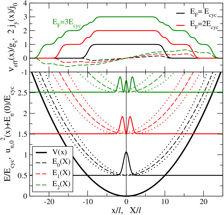
Figure 4: (color online) Lower part: potential $V(x)=(m^{*}/2)\Omega^{2}x^{2}$ for $\Omega/\omega_{c}=0.1$, resulting energy bands $E_{n}(X)$ for $n=0,\,1,\,2.$, and squared and shifted eigenfunctions at $X=0$. Energies are in units of the cyclotron energy $E_{\rm cyc}=\hbar\omega_{c}$ and lengths in units of the magnetic length $\ell$. Upper part: effective filling factor $\nu_{\rm eff}(x)$ (solid lines) and current density $j_{y}(x)$ (dashed lines, $j_{0}=g_{s}e\omega_{c}/(2\pi\ell)$) for three values of the Fermi energy, see text.

The upper part of Fig. 4 shows, for $k_{B}T=0.01\hbar\omega_{c}$ and three values of the electrochemical potential $\mu^{*}=E_{F}$, the electron and the current density, calculated according to Eqs. (12) and (13) with $f_{n,X}=f([E_{n}(X)-\mu^{*}]/k_{B}T)$. On the scale of the figure, the shown results cannot be distinguished from those calculated for $T=0$ and the same Fermi energies.

Transforming the $X$-integral into an integral over $\tilde{X}$ introduces a pre-factor $(\widetilde{\omega}/\omega_{c})^{2}$, which increases the density of effective center coordinates $\tilde{X}$ and thereby of eigenstates in each Landau band. Referring the effective filling factor to this enhanced density of states, $\nu_{\rm eff}(x)=2\pi\ell^{2}(\omega_{c}/\widetilde{\omega})^{2}n(x)$, leads to the results shown in Fig. 4, with plateau values equal to integer multiples of the spin-degeneracy $g_{s}$ in regions where the Fermi energy is well between two adjacent Landau bands. Note that in these regions the usually defined filling factor $\nu(x)=(\widetilde{\omega}/\omega_{c})^{2}\nu_{\rm eff}(x)>g_{s}(n_{\rm occ}+1)$ is larger than the number of fully occupied Landau bands with $n\leq n_{\rm occ}$.

The plateaus of the density profile are separated by broadened steps, which reflect the structure of the wavefunction of the highest, partly occupied band. Clearly the width of the density profile increases with increasing $E_{F}$, and, due the symmetry of the considered potential, the profiles are even functions of position. The current density $j_{y}(x)$, which is an odd function of position, is, similar to the density, the sum of the contributions of all (partly) occupied bands, and is determined by the current $e\Omega^{2}\tilde{X}/\omega_{c}$ carried by the state $|n,X\rangle$, and by its occupation. Of course, the total current in the considered thermal equilibrium state vanishes.

The calculation of the LDOS from Eq. (15) is also straightforward, with $\tilde{\xi}=x/\tilde{\ell}$ and $\tilde{\xi}_{n}^{\pm}(E)=\tilde{X}_{n}^{\pm}(E)/\tilde{\ell}$ we find

$$D(E;x)=\frac{g_{s}}{2\pi\ell^{2}}\frac{\widetilde{\omega}^{2}}{\Omega^{2}}\sum_{n,\pm}\frac{u_{n}^{2}\big{(}\tilde{\xi}-\tilde{\xi}_{n}^{\pm}(E)\big{)}}{\hbar\widetilde{\omega}\,|\tilde{\xi}_{n}^{\pm}(E)|}\,\theta_{n}(E),$$ (35)

where $\theta_{n}(E)=\theta\big{(}2E-\hbar\widetilde{\omega}(2n+1)\big{)}$ and $\tilde{X}_{n}^{\pm}(E)/\tilde{\ell}=\pm(\omega_{c}/\Omega)\sqrt{2E/(\hbar\widetilde{\omega})-(2n+1)}$. Of course $D(E;-x)=D(E;x)$ holds. The LDOS is shown for three different positions $x$ by the black lines in Fig. 5. Since for increasing

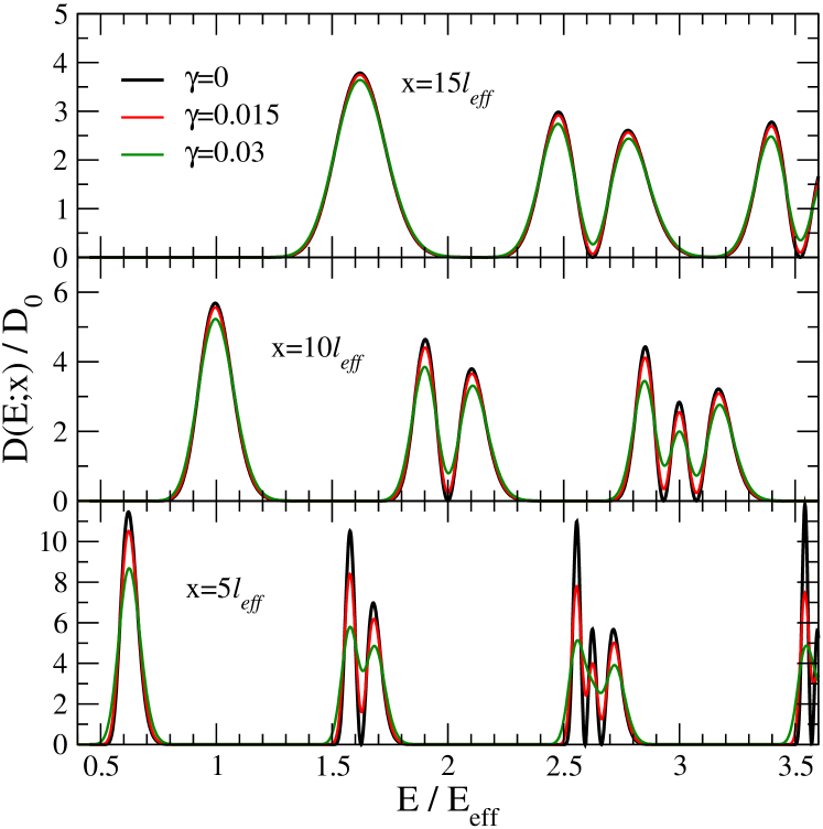
Figure 5: (color online) LDOS $D(E;x)$ for the parabolic confinement model with $\Omega/\omega_{c}=0.1$ at three positions, $x/\tilde{\ell}=5,\,10,\,15$. The black lines are without collision broadening, $\gamma=0$, Eq. (35). The colored lines are with collision broadening according to Eqs. (21) and (20) for $\gamma\equiv\Gamma/E_{\rm eff}=0.015$ and $0.03$. Energy in units of $E_{\rm eff}=\hbar\widetilde{\omega}$, position in units of $\ell_{\rm eff}=\tilde{\ell}$, $D_{0}=m^{*}/(\pi\hbar^{2})$, and $g_{s}=2$.

$|x|$ the contribution to the LDOS come from wavefunctions with increasing $|X|$, i.e., increasing values of energy dispersion $|dE_{n}(X)/dX|$, the contributions of the individual bands become broader and the gaps between these contributions become smaller, as can already be seen from Fig. 4. The gap between the contributions due to the lowest bands vanishes for $x/\tilde{\ell}\gtrsim 20$, i.e. if $\tilde{\ell}|dE_{n}(X)/dX|/\hbar\widetilde{\omega}\gtrsim 0.2$ holds for the relevant $X$-values. This condition is similar to that found in the linear-potential model.

Due to the vanishing energy dispersion in the center, $[dE_{n}(X)/dX](0)=0$, the contributions of all bands to $D(E;x)$ become very narrow and $\delta$-function-like for small values of $x$. With increasing distance from the center, the contributions become wider and clearly reflect the structure of the corresponding wavefunctions, notably their zeroes.

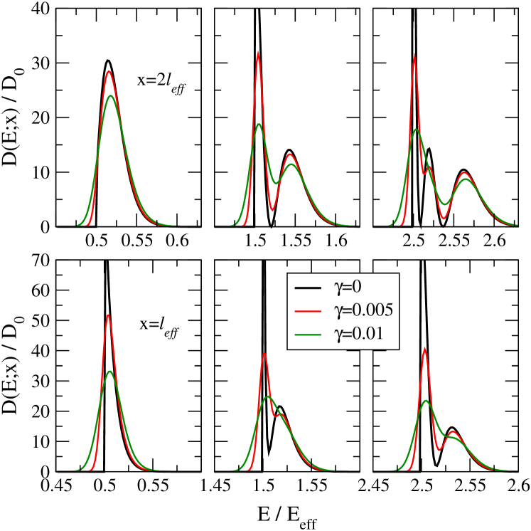
Figure 6: (color online) As in Fig. 5, but for smaller $x$ values and smaller damping. The lower three plots are for $x=\tilde{\ell}$, the upper three for $x=2\tilde{\ell}$. The gap regions are omitted.

Apparently in the energy range shown in Fig. 6 all the zeroes of the wavefunctions are reflected in the LDOS for $x=2\tilde{\ell}$, but not yet for $x=\tilde{\ell}$.

Figures 5 and 6 also show the effect of collision broadening on $D(E;x)$, which is most important for small $|x|$ values, where it completely washes out the internal structure of the individual contributions. For larger values of $|x|$ the collision broadening levels off the maxima and smears out the zeroes of the individual structures, and at large values, when these structures become broad, the collision broadening becomes relatively unimportant.

IV Model for incompressible stripes

In the screening theory of the IQHE in narrow Hall bars Guven03:115327 ; Siddiki04:195335 ; Gerhardts08:378 incompressible stripes (ISs) play an important role, which separate neighboring compressible regions, in which adjacent Landau levels are pinned to the Fermi energy, since these ISs offer the possibility of dissipationless current flow through an otherwise dissipative Hall bar. To understand the width and the separation of the QH plateaus, i.e. of the $B$-intervals in which the resistance quantization occurs, it is important to understand the conditions under which an IS can carry a dissipation-free current. The calculations Guven03:115327 ; Siddiki04:195335 were based on a local model for the conductivity tensor $\hat{\sigma}_{\rm loc}(x)$, which was obtained from the density-dependent conductivity tensor $\hat{\sigma}(n_{\rm el})$ of a homogeneous 2DES of density $n_{\rm el}$ by replacing this density by the local density $n(x)$ of the inhomogeneous system, $\hat{\sigma}_{\rm loc}(x)=\hat{\sigma}\big{(}n(x)\big{)}$. On ISs of finite width with constant integer filling factor the components of this $\hat{\sigma}_{\rm loc}(x)$ have the quantized values, and dissipationless transport is obtained, if the current is restricted to these ISs. It has been argued Siddiki04:195335 ; Gerhardts08:378 that the width of an IS must be sufficiently large, e.g., more than several times the spatial extent of typical wavefunctions near the edges of the IS, since otherwise wavefunctions from opposite sides of the IS would overlap and lead to quasi-elastic scattering across the IS. Such QUILLS processes Eaves86:346 would lead to dissipation, so that too narrow stripes between neighboring compressible regions cannot support the resistance quantization.

A suitable quantity containing quantitative information about the ability of an IS to carry dissipationless current should be the LDOS in the IS. To calculate this LDOS, we have to model the IS with some care. Even if the potential within the IS might be well approximated by a linear position dependence, at the interesting energies around the Fermi energy (i.e. the electrochemical potential) there exist nearby states of the compressible regions, which may contribute to the LDOS when its gap near the Fermi energy becomes small.

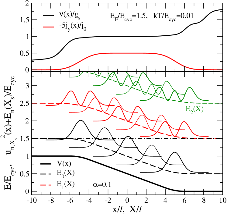
Figure 7: (color online) Upper part: filling factor $\nu(x)$ and current density $j_{y}(x)$, in units of $j_{0}=(g_{s}/2\pi)\,e\omega_{c}/\ell$; lower part: corresponding potential $V(x)$, energy eigenvalues $E_{n}(X)$ and squared eigenfunctions at center coordinates $X_{s}/\ell=0,\,\pm 2.46,\,\pm 4.92$, shifted upwards by $E_{n}(X_{s})/\hbar\omega_{c}$.

To get an idea how the LDOS changes with the width of an IS, we consider as a crude model the sum $V(x)=V_{S}(x)+V_{T}(x)$ of a smoothened step potential

$$V_{S}(x)=\hbar\omega_{c}\cdot\left\{\begin{array}[]{cc}1,&\xi<-\xi_{0},\\ 1-\kappa(\xi+\xi_{0})^{2},&-\xi_{0}<\xi<-\xi_{+},\\ \frac{1}{2}-\alpha\xi,&-\xi_{+}<\xi<\xi_{+},\\ \kappa(\xi-\xi_{0})^{2},&\xi_{+}<\xi<\xi_{0},\\ 0,&\xi_{0}<\xi,\end{array}\right.$$ (41)

and a weak linear potential $V_{T}(x)=0.1k_{B}T\xi$, with $\xi=x/\ell$. We take $\xi_{0}=(1-\gamma)/\alpha$, $\xi_{+}=\gamma/\alpha$, and $\kappa=\alpha^{2}/(2-4\gamma)$, with $0<\gamma\leq 1/2$, so that the fraction $2\gamma$ of the step height $\hbar\omega_{c}$ is bridged by the linear part of $V_{S}(x)$ and the total width of the stripe is $2\xi_{0}$. In the following we take $\gamma=0.4$ if we want to avoid sharp kinks in the potential, or $\gamma=0.5$, if we want to avoid the arbitrarily introduced smoothening by parabolic potential regions.

The weak linear term $V_{T}(x)$ is added to allow for a variation of the electron density in the regions $|x/\ell|>\xi_{0}$. The idea is to simulate the situation in compressible regions, where self-consistent screening leads to pinning of Landau levels to the Fermi energy, accompanied by a variation of the effective potential $V(x)$ of the order of $k_{B}T$.

IV.1 Thermal equilibrium

First we consider the system without imposed current in thermal equilibrium with constant electrochemical potential $\mu^{*}=E_{F}=1.5\hbar\omega_{c}$, so that for $X\ll-\ell$ the lowest energy band $E_{0}(X)$ approaches $E_{F}$ from below, and for $X\gg\ell$ the second band $E_{1}(X)$ approaches $E_{F}$ from above. Numerical solution of the eigenvalue problem for this potential $V(x)$ with $\alpha=0.1$ yields the energy bands and the electron and current densities presented in Fig. 7. The width ($\sim\ell/\alpha=10\ell$) of the IS is large enough to allow for an inner region with constant electron and current densities, similar to the gap regions of Fig. 3, which shows results for a linear potential with the same slope $dV/dx=eE_{x}=-0.1\hbar\omega_{c}/\ell$.

Figure 8: Energy dependence of the LDOS for the five indicated positions $x$. The broadened step potential is given by Eq. (41) with $\alpha=0.1$ (and $\gamma=0.4$, see text).

The corresponding LDOS is sketched in Fig. 8 for five characteristic values of the position $x$. In the center of the IS, at $x=0$, one finds the same LDOS as for the linear-potential model with the same electric field, see the lower panel of Fig. 1. As the position $x$ moves towards the edges of the IS and leaves the regime of linear potential, the individual contributions of the different bands become asymmetric and narrower, since the magnitudes of the slopes $|dE_{n}(X)/dX|$ become smaller.

For positive $x$-values the curvatures of potential and energy bands become positive, and the low-energy parts of the individual contributions are enhanced, while the high-energy parts are reduced, just as we found for the parabolic confinement potential in Fig. 5. For negative $x$-values the curvatures become negative and the asymmetry of the individual contributions is inverted, with reduced low-energy and enhanced high-energy parts.

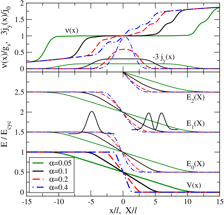
Figure 9: (color online) Lower part: Potential $V(x)=V_{S}(x)+V_{T}(x)$ and corresponding energy bands $E_{n}(X)$ for $\alpha$ parameters as indicated ($\gamma=0.4$). For $\alpha=0.1$ shifted squares of energy eigenfunctions are indicated. Upper part: corresponding filling factors and current densities, $E_{F}=1.5E_{\rm cyc}$, $k_{B}T=0.01E_{\rm cyc}$, $E_{\rm cyc}=\hbar\omega_{c}$.

For positions close to the high-energy edge of the IS ($x/\ell\approx-4.9$) there are many nearby states with lower energy, but nearly no states with slightly higher energies. As a consequence, the individual band-contributions to the LDOS for such $x$-values show a sharp high-energy cutoff. Similarly, near the low-energy edge of the IS ($x/\ell\approx 4.9$) we find low-energy cutoffs. For positions outside the IS ($|x/\ell|>\xi_{0}=6$) the individual band-contributions to the LDOS are extremely narrow and $\delta$-function-like, very similar to the bare Landau DOS.

Since for the screening theory of the IQHE the existence of incompressible stripes of finite width is crucial, we present in Fig. 9 for potential steps of different steepness the resulting energy bands and the electron density and current density profiles. Density plateaus with integer filling factor $\nu(x)=g_{s}$ are obtained for $\alpha\lesssim 0.1$. For $\alpha\gtrsim 0.2$ the potential increase is so steep that it does not lead to a stripe of constant filling factor. Then it makes no longer sense to address the step region between the flat parts of the potential as incompressible stripe. If we assume that the critical steepness is close to $\alpha=0.15$, ISs do not exist if the width of the potential steps is not larger than $\sim 7\ell$, which is a little larger than the extent of the low-energy wavefunctions.

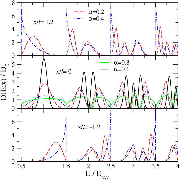
Figure 10: (color online) LDOS at three positions for several steepness parameters $\alpha$.

Figure 10 demonstrates how the LDOS behaves in this limit. The positions $|x/\ell|=1.2$ are for $\alpha=0.2$ well inside the stripe in the region of weak curvature, and one sees a similar behavior of the LDOS as for $|x/\ell|=2.46$ in Fig. 8. For $\alpha=0.4$, on the other hand, $|x/\ell|=1.2$ is at the edge of the stripe and the situation similar to that for $|x/\ell|=4.92$ in Fig. 8. The situation in the center of the stripe, at $x=0$, is not so easy to interpret. For $\alpha=0.2$ the contributions of the individual bands to the LDOS are broader than for $\alpha=0.1$, as indicated in Fig. 10, but they are still separated by well developed gaps, although according to Fig. 9 no IS exists. If we increase $\alpha$ further, the gaps shrink, but the LDOS vanishes at the energies $E=\hbar\omega_{c}(n+1/2)$, even if the potential step becomes very narrow. The reason is simple: slightly below $E=1.5\,\hbar\omega_{c}$ there are nearby states in the band $E_{0}(X)$ and slightly above there are nearby states of the band $E_{1}(X)$. But as the energy approaches $E=1.5\hbar\omega_{c}$, the center coordinates of these states move away from $X=0$ and the value of their wavefunctions at $x=0$ becomes exponentially small.

This behavior of the LDOS in the center of the IS makes the definition of an overlap of the contribution of adjacent Landau levels as a criterion for the vanishing of the gap in the thermal equilibrium situation useless. Things change, however, if we consider a situation with imposed current.

IV.2 Imposed Hall current

We now consider an externally imposed current along the system and assume (nearly) perfect screening. The current is accompanied by a Hall potential $V_{H}(x)$, which as a consequence of screening is constant in the compressible regions and therefore must drop over the region of the potential step. Self-consistent screening calculations Guven03:115327 show that the width of the incompressible stripes is changed by the applied current. It becomes larger, if applied and intrinsic current have the same direction, and the width becomes smaller, if applied and intrinsic currents have opposite directions.

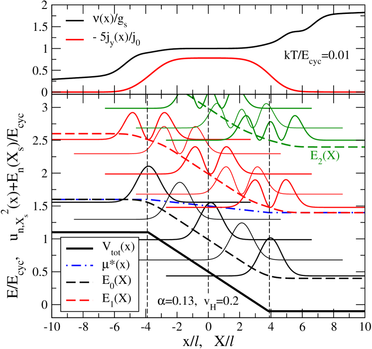
Figure 11: (color online) Lower part: Total potential, corresponding energy bands, electrochemical potential, and squared and shifted energy eigenfunctions for $X_{s}/\ell=0,\,\pm 1.98,\,\pm 3.90$. Upper part: corresponding filling factors and current densities. Parameters $\alpha=0.13$, $v_{H}=V_{H}^{0}/\hbar\omega_{c}=0.2$, see text.

Here we will not consider these details and make the simplifying assumption that the total potential $V_{\rm tot}(x)=V(x)+V_{H}(x)$ and the electrochemical potential $\mu^{*}(x)$ are constant in the compressible regions $|x/\ell|>\xi_{0}$ and vary linearly in the stripe region, i.e., we put in Eq. (41) $\gamma=0.5$ and $\xi_{0}=\xi_{+}=1/(2\alpha)$, and thus suppress the quadratic region. To be specific, we take $V_{H}(x)=V_{H}^{0}\,F(x/\ell;\xi_{0})$ with

$$F(\xi,\xi_{0})=\left\{\begin{array}[]{cc}\frac{1}{2},&\xi\leq-\xi_{0},\\[2.84544pt] -\alpha\xi,&|\xi|<\xi_{0},\\[2.84544pt] -\frac{1}{2},&\xi\geq\xi_{0},\end{array}\right.$$ (45)

as Hall potential, $V_{\rm tot}(x)=V_{H}(x)+\hbar\omega_{c}[1/2+F(x/\ell;\xi_{0})]$ as total potential, and $\mu^{*}(x)=1.5\hbar\omega_{c}+V_{H}(x)$ as electrochemical potential. Numerical results for energy bands, wavefunctions, electron and current density are presented in Fig. 11 for $\alpha=0.13$ and $V_{H}^{0}=0.2\hbar\omega_{c}$. Although the potential has sharp kinks near $x=\pm 3.9\ell$, the energy bands $E_{n}(X)$ are smooth and the curvatures near $X=\pm 3.9\ell$ become smaller with increasing $n$. In the linear regime near $x=0$ the centers of the wavefunctions $\varphi_{n,X}(x)$ are shifted from $X$ to larger values, as expected from Eq. (23). Near $x=3.9\ell$, where the potential kink can be considered as limit of a positive curvature, the wavefunctions are somewhat narrower than near $x=0$. This is immediately understood from Eq. (34) and a parabolic approximation of the potential near the kink. Similarly, near $x=-3.9\ell$, where the potential kink corresponds to a negative curvature, the wavefunction are somewhat wider than near $x=0$.

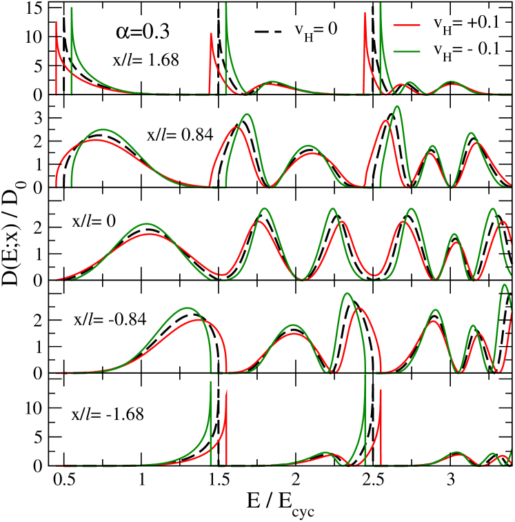
Figure 12: (color online) LDOS $D(E;x)$ for a steep potential step, $\alpha=0.3$, with and without externally imposed current, for five positions $x$ as indicated. Strength and direction of the imposed currents are characterized by the corresponding Hall potentials $v_{H}=V_{H}^{0}/\hbar\omega_{c}$ with values $0,\,\pm 0.1$ as indicated.

The most important consequence of the imposed current is that the corresponding Hall potential leads to an energetic overlap of the high-energy edge of the lowest energy band $E_{0}(X)$ and the low-energy edge of the next band $E_{1}(X)$. Thus the situation near $x=0$ is similar to that in the linear-potential model, and the individual band-contributions to the LDOS will overlap, if the region of the potential step will become to narrow. If the external current is applied in the opposite direction to that of the intrinsic current, the sign of $V_{H}(x)$ will change and, instead of an overlap of the bands, a finite energy gap between the bands will result. This will lead to energy gaps in the LDOS at $x=0$, which will remain even if the width of the potential step will become small.

These results for the LDOS are illustrated in Fig. 12, where we consider a steep potential step, $\alpha=0.3$, which does not allow for a IS with constant density in the step region. Without imposed current, $v_{H}=0$, the LDOS at $x=0$ has no gaps, but has very small values in the middle $E_{n,n+1}=[E_{n}(0)+E_{n+1}(0)]/2$ between the band energies $E_{n}(X)$ at $X=0$, $D(E_{n,n+1};0)\approx 0$. If a current in the direction of the intrinsic current is imposed, $v_{H}=0.1$, these values increase drastically and a considerable overlap of the contribution due to adjacent bands is observed. If the current is imposed in the opposite direction, $v_{H}=-0.1$, well developed gaps occur around the energies $E_{n,n+1}$, in which $D(E;0)$ vanishes. On the other hand, the density profile, which is not shown, changes only very little due to the applied current and remains without any flat part in the step region for both directions of the imposed current, similar to the profiles shown in the upper part of Fig. 9 for $\alpha\geq 0.2$.

Figure 13 demonstrates how gaps and overlap, respectively, of the LDOS $D(E;x)$ in the center of the potential step, $x=0$, depend on the steepness of the potential and on the Hall potential.

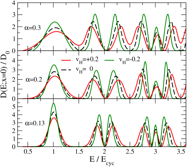
Figure 13: (color online) LDOS $D(E;x=0)$ for three value of the steepness, $\alpha=0.13,\,0.2,\,0.3$ and three values of the Hall voltage, $v_{H}=V_{H}^{0}/\hbar\omega_{c}=0,\,\pm 1$, as indicated.

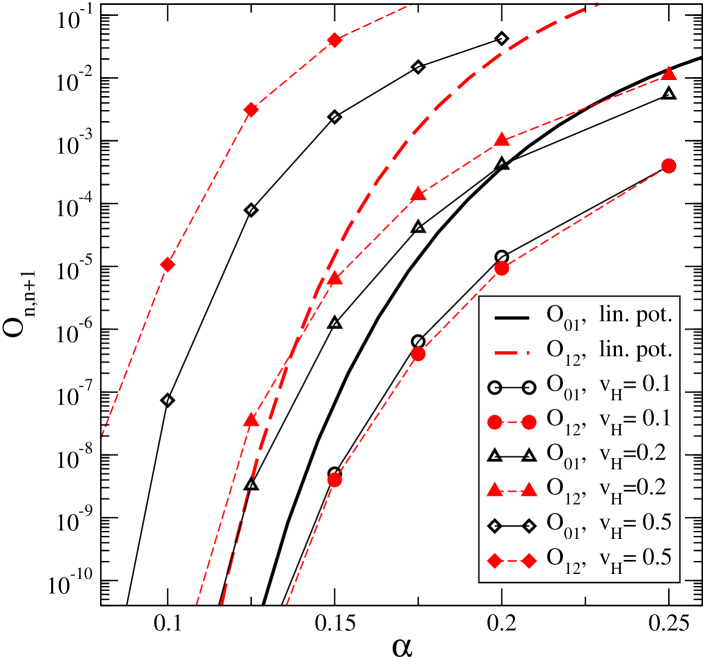
Figure 14: (color online) Overlaps $O_{01}$ and $O_{12}$ as functions of the potential steepness $\alpha$ for different value of the reduced Hall voltage $v_{h}=V_{H}^{0}/\hbar\omega_{c}$, as indicated by the symbols. The lines between the symbols are guides to the eye. The heavy lines indicate the corresponding results for the linear-potential model, shown in Fig. 2 for $\eta\equiv\alpha$.

For $V_{H}^{0}<0$ we observe well developed gaps, even if the potential step is so steep, that no IS exists ( see Fig. 9). For $V_{H}^{0}>0$, i.e. imposed and intrinsic current in the same direction, we have a situation as in the linear-potential model, and we can consider the overlap as a function of the potential steepness, as in Fig. 2. Generalizing Eq. (26) by

$$O_{n,n+1}=D_{n}(E_{n,n+1};0)D_{n+1}(E_{n,n+1};0)/D_{0}^{2},$$ (46)

where the $D_{n}(E;x)$ are the individual band contributions to $D(E;x)=\sum_{n}D_{n}(E;x)$ defined in Eq. (15). Results are shown in Fig. 14.

V Remarks and conclusion

We have simplified and extended previous calculations of the LDOS of a Landau quantized 2DES in the presence of a constant, unidirectional in-plane electric field, Kramer04:21 ; Kramer06:1243 and we have shown that the LDOS in principle is a useful concept for further calculations, if the occupation probability of energy eigenstates depends only on their energy eigenvalues but not on other conserved quantities. We have also considered the case of a homogeneous 2DES supporting a homogeneous dissipation-free Hall current, which can be described by the standard methods of grand-canonical equilibrium Oh97:13519 but not in terms of the LDOS. For this linear-potential model we have also quantified the overlap of adjacent band contributions to the LDOS, which leads to a closing of gaps in its energy-dependence and indicates the onset of quasi-elastic inter-Landau-level scattering (QUILLS). In realistic situations QUILLS will lead to a breakdown of the IQHE, e.g., under high externally imposed currents. To get more than an indication of the onset of such breakdown effects, one should, however, explicitly consider electron-impurity scattering under these conditions, which goes far beyond the mere calculation of the LDOS of the idealized 2DES. Here we have considered only a simple phenomenological treatment of collision broadening and mentioned that this is not sufficient under strong electric fields. Future work on the necessary generalization of the treatment of collision broadening, even within the frame of the self-consistent Born approximation, seems desirable.

To get a better understanding of the behavior of the LDOS in other situations than the simple linear-potential model, we have considered a parabolic potential as a model for a laterally confined 2DES, which also allows analytical calculation of the LDOS, Eq. (35). Whereas $D(E;x)$ at $x=0$ exhibits one-over-square-root singularities of the type $1/\sqrt{E-E_{n}(0)}$ at the energies $E>E_{n}(0)$, for $|x|>0$ there are no singularities but, due to the increasing electric field strength, the individual band contributions to the LDOS become asymmetric and broader with increasing $|x|$.

Finally we have calculated the LDOS for incompressible stripes, which are an essential ingredient of the screening theory of the IQHE. Guven03:115327 ; Siddiki04:195335 ; Gerhardts08:378 We use a simplified model of such an IS, which describes the compressible regions (CRs) next to the stripe by nearly constant potentials, and the stripe region in between by a more or less linear potential. One expects that, without collision broadening, the LDOS in the CRs approaches the singular Landau DOS, whereas in the linear-potential regions of incompressible stripes the situation should be similar to that in the linear-potential model considered in sect. III.1. In the transition regions between nearly constant and linear potential the results should be comparable with those for the parabolic-potential of sect. III.2. Concerning the energy dependence of the LDOS at characteristic positions $x$ we find these expectations confirmed. However, the closing of energy gaps and the onset of overlap of contributions from adjacent bands, which we interpreted in the linear-potential model of sect. III.1 as indication for the breakdown of the IQHE, are now more subtle and not so easy to interpret. In the center of the stripe region at $x=0$, the energy gaps become smaller as the distance between the CRs decreases and at the energies above and below the Fermi energy the centers of the energy eigenfunctions move towards the center of the stripe region. But exactly at the Fermi energy, which separates the lowest energy bands $E_{0}(X)$ and $E_{1}(X)$, there are no nearby states and $D(E_{F};0)\approx 0$ even if the CRs come so close that, due to the finite extent of the wavefunctions, no genuine IS with constant local filling factor $\nu(x)=g_{s}$ in an $x$-interval of finite width exists. The situation becomes clearer, if one imposes an external current on the system. This leads to a Hall potential in the stripe region, which may increase or diminish the intrinsic potential variation across the stripe region. If the imposed current has the same direction as the intrinsic one, the potential variation increases and around $E_{F}$ the two lowest bands overlap energetically. Then the situation is as in the linear-potential model of sect. III.1, and the overlap criterion for the breakdown of the IQHE can be applied. If imposed and intrinsic currents have opposite directions, the potential variation across the strip region decreases and at $E_{F}$ a gap opens between the two lowest bands. Then in $D(E;0)$ an energy gap of finite width around $E=E_{F}$ remains, even if the distance between the CRs becomes so small that, the stripe region between them can no longer support a dissipationless current, i.e. support the IQHE. Of course, in a real sample both situations occur simultaneously, since the intrinsic currents in the stripe regions of opposite sides of the sample have opposite directions. Within the screening theory of the IQHE one finds that the width of the incompressible stripes is different in both situations. If imposed and intrinsic currents have the same direction, the stripe is wider than in the opposite case, Guven03:115327 ; Gerhardts08:378 however, to determine the widths of the stripes and to decide whether they can support the IQHE requires an involved self-consistent calculation.

In summary, the LDOS is an interesting concept, is easy to evaluate, and can give some hints on possible scattering effects, such as QUILLS, which may lead to the breakdown of the IQHE. However, to really understand the IQHE is much more complicated and requires non-trivial calculations. One should include the relevant scattering effects, which usually lead to dissipative transport, and find out, under which conditions they become ineffective and lead to the peculiar transport phenomena observed in the plateau regime of the IQHE.

- (1) K. v. Klitzing, G. Dorda, and M. Pepper, Phys. Rev. Lett. 45, 494 (1980).
- (2) R. E. Prange and S. M. Girvin, in The Quantum Hall Effect (Springer, New York, 1987).
- (3) B. Kramer, S. Kettemann, and T. Ohtsuki, Physica E 20, 172 (2003).
- (4) H. Bachmair, E. O. Göbel, G. Hein, J. Melcher, B. Schumacher, J. Schurr, L. Schweitzer, and P. Warnecke, Physica E 20, 14 (2003).
- (5) A. Siddiki, J. Horas, J. Moser, W. Wegscheider, and S. Ludwig, Europhysics Letters 88, 17007 (2009).
- (6) B. I. Halperin, Phys. Rev. B 25, 2185 (1982).
- (7) M. Büttiker, Phys. Rev. Lett. 57, 1761 (1986).
- (8) D. B. Chklovskii, B. I. Shklovskii, and L. I. Glazman, Phys. Rev. B 46, 4026 (1992).
- (9) A. L. Efros, Solid State Commun. 65, 1281 (1988).
- (10) A. L. Efros, Solid State Commun. 67, 1019 (1988).
- (11) D. B. Chklovskii, K. A. Matveev, and B. I. Shklovskii, Phys. Rev. B 47, 12605 (1993).
- (12) K. Lier and R. R. Gerhardts, Phys. Rev. B 50, 7757 (1994).
- (13) J. H. Oh and R. R. Gerhardts, Phys. Rev. B 56, 13519 (1997).
- (14) P. Weitz, E. Ahlswede, J. Weis, K. v. Klitzing, and K. Eberl, Physica E 6, 247 (2000).
- (15) E. Ahlswede, P. Weitz, J. Weis, K. von Klitzing, and K. Eberl, Physica B 298, 562 (2001).
- (16) E. Ahlswede, J. Weis, K. von Klitzing, and K. Eberl, Physica E 12, 165 (2002).
- (17) K. Güven and R. R. Gerhardts, Phys. Rev. B 67, 115327 (2003).
- (18) A. Siddiki and R. R. Gerhardts, Phys. Rev. B 70, 195335 (2004).
- (19) R. R. Gerhardts, phys. stat. sol. (b) 245, 378 (2008).
- (20) A. Siddiki, J. Horas, D. Kupidura, W. Wegscheider, and S. Ludwig, New Journal of Physics 12, 113011 (2010).
- (21) L. Eaves and F. W. Sheard, Semicond. Sci. Technol. 1, 346 (1986).
- (22) K. Güven, R. R. Gerhardts, I. I. Kaya, B. E. Sagol, and G. Nachtwei, Phys. Rev. B 65, 155316 (2002).
- (23) T. Kramer, C. Bracher, and M. Kleber, Journal of Optics B: Quantum and Semiclassical Optics 6, 21 (2004).
- (24) T. Kramer, International Journal of Modern Physics B 20, 1243 (2006).
- (25) H. Scher and T. Holstein, Physical Review 148, 598 (1966).
- (26) H. Keiter, Z Physik 198, 215 (1967).
- (27) E. Bangert, Z. Physik 215, 177 (1968).
- (28) R. R. Gerhardts, Z. Physik B 22, 327 (1975).
- (29) M. Abramowitz and I. A. Stegun, in Handbook of Mathematical Functions (Dover Publications, New York, 1964).
- (30) T. Ando, A. B. Fowler, and F. Stern, Rev. Mod. Phys. 54, 437 (1982).
- (31) R. R. Gerhardts, Z. Physik B 21, 285 (1975).
- (32) Y. Y. Wei, J. Weis, K. v. Klitzing, and K. Eberl, Appl. Phys. Lett. 71, 2514 (1997).
- (33) Y. Y. Wei, J. Weis, K. v. Klitzing, and K. Eberl, Physica B 249-251, 496 (1998).