Work distribution for the driven harmonic oscillator with time-dependent strength: Exact solution and slow driving
Abstract
We study the work distribution of a single particle moving in a harmonic oscillator with time-dependent strength. This simple system has a non-Gaussian work distribution with exponential tails. The time evolution of the corresponding moment generating function is given by two coupled ordinary differential equations that are solved numerically. Based on this result we study the behavior of the work distribution in the limit of slow but finite driving and show that it approaches a Gaussian distribution arbitrarily well.
pacs:
05.40.-a, 05.70.Ln1 Introduction
Driving a system away from thermal equilibrium requires work. Since thermal fluctuations play a paramount role in small, mesoscopic systems it is only consequent to also define a fluctuating work along single trajectories [1, 2]. While the celebrated Jarzynksi [3] and Crooks [4, 5] non-equilibrium work relations constrain the possible shapes, the actual distribution of the work is still a non-universal function that depends on both the system dynamics and the driving protocol. Analytical expressions for the work distribution in isothermal processes are rather scarce except when the distribution is exactly a Gaussian [6]. In particular, a single Brownian particle in a moving harmonic potential has been studied extensively both theoretically [7, 8, 6, 9] and experimentally [10, 11] by trapping a colloidal particle with optical tweezers.
The direct application of the Jarzynski relation to numerical or experimental data in order to extract equilibrium free energy differences is marred by the fact that it falls into the class of biased estimators. Rare, untypical trajectories with low work values are exponentially weighted and a large number of observations is required for estimates to converge. This number typically grows exponentially with the mean dissipated work. Two principal schemes have been discussed to address this problem: (i) reduction of the mean dissipation by using optimal protocols [12] or escorted simulations [13]; (ii) unbiased estimators based on Bennett’s acceptance ratio method [14] or extended bridge sampling [15].
Of course, the easiest method to reduce the mean dissipated work might still be to reduce the driving speed and keep the system close to equilibrium. In this case a Gaussian has been predicted [16, 17] as the limit distribution for the work. However, as has been noted many times, a naive application of a truncated Gaussian work distribution leads to wrong results for the free energy difference (see, e.g., the discussion in Ref. [18]). While the central limit theorem predicts that the center of the distribution approaches a Gaussian this does not necessarily apply to the extreme tails of the distribution, which are crucial for the correct determination of free energy changes. For practical purposes it is, therefore, important to understand the convergence of the work distribution towards its limiting Gaussian distribution.
In this paper we study the probably simplest system that leads to a non-Gaussian distribution of work: a single Brownian particle moving in a one-dimensional, tightening harmonic potential. In addition to an exponential tail for large work values the probability for negative work values is exactly zero. Instead of determining the distribution of work directly we consider its moment generating function and obtain a closed set of non-linear ordinary differential equations. Using this exact result allows us to study the work distribution as we reduce the driving speed.
2 Work distribution and its generating function
We consider a particle with position moving in a harmonic potential
| (1) |
with time-dependent strength . Assuming overdamped dynamics the evolution of the probability distribution is well described by the Fokker-Planck equation
| (2) |
Here and throughout the paper we measure energy in units of with Boltzmann’s constant , length in units of , and time in units of . The free diffusion coefficient of the particle is , and is the initial non-dimensionless value of the trap strength (i.e., from now on ). Given a driving protocol from to the work is defined as the functional
| (3) |
with switching time . In particular, for () the work is always non-negative (non-positive).
Since is the result of a stochastic process the work also will be a random variable with distribution . For any driving protocol the Jarzynski relation
| (4) |
provides the link between non-equilibrium work and the equilibrium change of free energy , which for the system studied here becomes
| (5) |
For the analytical study of work distributions it has turned out to be convenient to consider the joint probability to find the system in state at time and to have spent the accumulated work so far. Its time evolution is governed by
| (6) |
In the following we work with the Laplace transform
| (7) |
For simplicity we focus on . After one integration by parts and using we obtain from (6) the evolution equation
| (8) |
This is a linear reaction-diffusion type equation, called a ’sink’ equation, where diffusion is governed by the operator and ’probability’ is created or annihilated with a rate proportional to , i.e., the function is not normalized. Rather, its integral is the moment generating function
| (9) |
In particular, the mean and variance are obtained as
| (10) |
where .
Already in one of the first experiments demonstrating a non-equilibrium work relation [19] it has been noted that the distribution for the work is distinctly non-Gaussian. More recent computer simulations have found exponential tails for large [20, 21]. Indeed, considering the extreme case of instantaneously switching from to at some arbitrary time the work spent is . The work distribution, therefore, becomes
| (11) |
where we have averaged over the equilibrium distribution
The generating function reads
| (12) |
As a signature of the exponential tail diverges for with .
The other limiting case is that of a quasi-static process with and work distribution , implying the generating function
| (13) |
As a third exact result we note that for
| (14) |
solves the sink equation (8). The generating function obeys the Jarzynski relation, cf. (9) with (4). This particular solution to the sink equation (8) has been discussed first by Hummer and Szabo [22].
3 Time evolution of the generating function
From Eqs. (8) and (9) we obtain the equation of motion
after integration over , where
| (15) |
is the generalized second moment. Multiplying (8) by and integrating again over results in
By following this scheme we obtain a hierarchy of coupled ordinary differential equations. Fortunately, for the harmonic oscillator a closure can be found as follows. For we observe that the solution (14) is a, albeit not normalized, Gaussian. Since otherwise is not special we conclude that is a Gaussian for all . Then the closure
| (16) |
follows from Gaussian statistics, expressing the generalized fourth moment in terms of the functions and . The resulting system of non-linear, first-order ordinary differential equations
| (17) |
is our first main result. Through inserting the Gaussian ansatz
into equation (8) it is straightforward to check that (17) is indeed correct. Augmented by the initial conditions these equations are readily solved numerically by standard techniques.

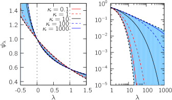
In figure 1 we plot the generating function at the final value of the control parameter for different driving speeds using the linear protocol
| (18) |
The second relation fixes the switching time . In the right panel of figure 1 the generating function for large is shown. The probability to have spent no work is related to this asymptotic behavior through the initial value theorem,
The numerical results suggest that even for large driving speeds decays faster than with and only for instantaneous switching , see equation (11). For large an exponential tail is expected [21], which corresponds to a divergence of at . Starting from we expect a singularity at time for all , where corresponds to . Together with the results Eqs. (12) and (13) for the two limiting cases this implies a value for that moves from to with decreasing driving speed .
4 Slow driving
Of greater practical importance than quasi-static driving with are processes with slow but finite driving speed . In this case a Gaussian distribution for the work has been predicted [17]. Of course, in the present situation the work distribution can never be strictly a Gaussian since and because of the existence of an exponential tail for large .
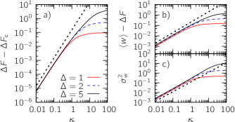
We calculate the true mean and variance [see (10)] by integrating the four coupled equations
which follow from (17) after expanding and . Truncation of the cumulant expansion for the free energy leads to the approximation
| (19) |
In figure 2a) the difference is plotted as a function of the driving speed for the linear protocol (18). It shows that the difference vanishes as and that, therefore, the true free energy can be arbitrarily well approximated by equation (19) through lowering the driving speed . In figure 2b) and c) the mean dissipated work and variance are shown, respectively.

The strategy used in Ref. [17] to obtain the work distribution for slow driving corresponds to expanding the generalized second moment
| (20) |
in powers of . To first order we obtain from (17) , which is solved by the quasi-static solution (13). For the next order we plug the expansion (20) into (17) and retain only terms of order with . The result is
with
The generating function now reads
| (21) |
The corresponding distribution is of course a Gaussian with variance and mean , where
| (22) |
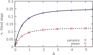
In contrast to the truncated Gaussian distribution obtained by using the true mean and variance, the distribution following from (21) always fulfills the Jarzynski relation (4). In figure 3 we compare the initial linear slope of mean and variance for these two Gaussian distributions, where the slope of the numerical data has been determined through a polynomial fit. The agreement between the two Gaussian distributions is our second main result.

5 Conclusions
For a driven harmonic oscillator we have derived the equation of motion for the moment generating function of the work distribution. Even though the exact distribution is non-Gaussian it can be approximated by a Gaussian such that the error vanishes with the square of the driving speed . While such a behavior is expected to hold in general [17] it remains to be investigated to which extent the exponent 2 is system dependent. We have focused on a linear protocol with which corresponds to a stiffening trap. The case follows in analogy by defining the Laplace transform in (7) with respect to negative work values. However, it should be kept in mind that slow driving is defined with respect to the time-scale separation between driving speed and the system’s relaxation time , which for a widening trap increases strongly.
The extension to a time-dependent quadratic potential energy with many degrees of freedom is straightforward through using the Wick theorem in (16). It will be worthwhile to study the method employed in this paper for more complicated potentials . While in the present case the Gaussian closure is exact, approximate closures for other potentials might nevertheless lead to accurate results for the work probability and cumulants.
References
References
- [1] K. Sekimoto, Prog. Theor. Phys. Supp. 130, 17 (1998).
- [2] U. Seifert, Eur. Phys. J. B 64, 423 (2008).
- [3] C. Jarzynski, Phys. Rev. Lett. 78, 2690 (1997).
- [4] G. E. Crooks, Phys. Rev. E 60, 2721 (1999).
- [5] G. E. Crooks, Phys. Rev. E 61, 2361 (2000).
- [6] T. Speck and U. Seifert, Eur. Phys. J. B 43, 521 (2005).
- [7] O. Mazonka and C. Jarzynski, arXiv:cond-mat/9912121 (1999).
- [8] R. van Zon and E. G. D. Cohen, Phys. Rev. E 67, 046102 (2003).
- [9] A. Imparato, L. Peliti, G. Pesce, G. Rusciano, and A. Sasso, Phys. Rev. E 76, 050101 (2007).
- [10] V. Blickle, T. Speck, L. Helden, U. Seifert, and C. Bechinger, Phys. Rev. Lett. 96, 070603 (2006).
- [11] D. Andrieux, P. Gaspard, S. Ciliberto, N. Garnier, S. Joubaud, and A. Petrosyan, Phys. Rev. Lett. 98, 150601 (2007).
- [12] T. Schmiedl and U. Seifert, Phys. Rev. Lett. 98, 108301 (2007).
- [13] S. Vaikuntanathan and C. Jarzynski, Phys. Rev. Lett. 100, 190601 (2008).
- [14] D. Collin, F. Ritort, C. Jarzynski, S. Smith, I. Tinoco, and C. Bustamante, Nature 437, 231 (2005).
- [15] D. D. L. Minh and J. D. Chodera, J. Chem. Phys. 131, 134110 (2009).
- [16] D. A. Hendrix and C. Jarzynski, J. Chem. Phys. 114, 5974 (2001).
- [17] T. Speck and U. Seifert, Phys. Rev. E 70, 066112 (2004).
- [18] G. E. Crooks and C. Jarzynski, Phys. Rev. E 75, 021116 (2007).
- [19] D. M. Carberry, J. C. Reid, G. M. Wang, E. M. Sevick, D. J. Searles, and D. J. Evans, Phys. Rev. Lett. 92, 140601 (2004).
- [20] C. Kwon, J. D. Noh, and H. Park, arXiv:1102.2973v1 (2011).
- [21] D. Nickelsen and A. Engel, arXiv:1102.4505v1 (2011).
- [22] G. Hummer and A. Szabo, Proc. Natl. Acad. Sci. U.S.A. 98, 3658 (2001).