Dynamic Critical Behavior of the Chayes–Machta Algorithm
for the Random-Cluster Model
I. Two Dimensions
Abstract
We study, via Monte Carlo simulation, the dynamic critical behavior of the Chayes–Machta dynamics for the Fortuin–Kasteleyn random-cluster model, which generalizes the Swendsen–Wang dynamics for the -state Potts ferromagnet to non-integer . We consider spatial dimension and in steps of , on lattices up to , and obtain estimates for the dynamic critical exponent . We present evidence that when the Ossola–Sokal conjecture is violated, though we also present plausible fits compatible with this conjecture. We show that the Li–Sokal bound is close to being sharp over the entire range , but is probably non-sharp by a power. As a byproduct of our work, we also obtain evidence concerning the corrections to scaling in static observables.
Key Words: Random-cluster model, Potts model, Chayes–Machta algorithm, Swendsen–Wang algorithm, cluster algorithm, dynamic critical behavior.
1 Introduction
Since nontrivial models in statistical mechanics are rarely exactly solvable, Monte Carlo (MC) simulations have become a standard tool for obtaining information on phase diagrams and critical exponents [1, 2, 3]. Unfortunately, MC simulations typically suffer from severe critical slowing-down [4, 5], so that the computational efficiency tends rapidly to zero as the critical point is approached. More precisely, the autocorrelation (relaxation) time diverges in the critical limit, most often like , where is the spatial correlation length. The dynamic critical exponent depends on both the model being investigated and the MC algorithm being used. For local algorithms one typically has .
An important advance was made in 1987 with the invention of the Swendsen–Wang (SW) cluster algorithm [6] for simulating the ferromagnetic -state Potts model [7, 8, 9] at integer . The SW algorithm is based on passing back and forth between the Potts spin representation and the Fortuin–Kasteleyn (FK) bond representation [10, 11, 12, 13, 14, 15]. More precisely, one introduces a joint probability distribution [14] of spin and bond variables, whose marginal on the spins (integrating out the bonds) is the Potts spin model and whose marginal on the bonds (integrating out the spins) is the FK random-cluster model [15]; one then updates this joint distribution by alternately applying the two conditional distributions (see Section 2.1 below for details).
Since a local move in one set of variables can have highly nonlocal effects in the other, it is not surprising that the SW algorithm might have less critical slowing-down than the conventional local algorithms. And this is in fact the case: although the SW algorithm does not eliminate critical slowing-down, it does radically reduce it compared to local algorithms. Much effort has therefore been devoted, for both theoretical and practical reasons, to understanding the dynamic critical behavior of the SW algorithm as a function of the spatial dimension and the number of Potts spin states. The best information on the dynamic critical exponent prior to the present work is summarized in Table 1. Unfortunately, it is very difficult to develop a physical understanding from the small number of non-trivial “data points” at our disposal: second-order non-mean-field transitions occur only for and .111 A continuous (second-order) transition occurs also in the Ising () model in dimensions , but here the static behavior is mean-field. One expects the dynamic critical exponents likewise to be dimension-independent for (with possible multiplicative logarithmic corrections at ).
| Estimates of | ||||
|---|---|---|---|---|
| 0 | 0 | 0 | 0 | |
| 0 | () | |||
| 0 | — | — | ||
| 0 | () | — | — | |
A further advance was made in 1998 by Chayes and Machta (CM) [25], who devised a cluster algorithm for simulating the FK random-cluster model at any real value . The idea behind the CM algorithm is very similar to that of SW, but now one starts with the random-cluster (bond) measure and introduces auxiliary color (spin) variables on the sites, so that we again have a joint model of spins and bonds, analogous to the one employed in the SW algorithm. Although the marginal measure on the spins no longer has any obvious physical interpretation when is noninteger, the joint measure can still be used to construct an efficient cluster algorithm, by alternately applying the conditional distributions exactly as in standard SW. The CM algorithm thus generalizes the SW algorithm and in fact reduces to (a slight variant of) it when is an integer: see Section 2.2 for details. Indeed, the CM algorithm can be thought of as a “natural” interpolation of the SW algorithm to noninteger (though unfortunately only for ). Thus, by using the CM algorithm we can study the dynamic critical behavior of the SW–CM dynamic universality class as a function of the continuous variable throughout the range , where is the maximum for which the transition is second-order on the given lattice .222 We stress that is not necessarily the same for all lattices of a given dimension ; the first-order or second-order nature of the transition is a non-universal question. See [26] for further discussion. For the standard two-dimensional lattices (square, triangular and hexagonal) we have . This vastly enhances our ability to make theoretical sense of the numerical results.
In the present paper we perform high-precision MC simulations of the random-cluster model on the square lattice (), for in steps of , using the CM algorithm. Our main goal is to gain better insight into the SW–CM dynamic universality class in two dimensions by studying the behavior as a function of the continuous variable . We estimate numerically several dynamic critical exponents for each value of , and we attempt to understand their behavior as a function of . As a byproduct we also obtain new information on corrections to scaling in the static quantities. In the companion paper [27] we carry out an analogous study for the simple-cubic lattice () at ; and in a forthcoming paper [28] we will analyze the case of the complete graph (Curie–Weiss model).333 A brief summary of the preliminary results in this trio of papers has appeared in letter form [29].
One advantage of considering is of course is that we have available a remarkable amount of information concerning the static behavior of the random-cluster model as a function of . This information includes the exact location [30, 31] of the transition point on the square lattice, namely , and the knowledge that the transition is second-order for and first-order for . Furthermore, the leading and next-to-leading thermal and magnetic critical exponents are known exactly (though non-rigorously) for the entire range [32, 33, 34]:
| (1.1) | |||||
| (1.2) | |||||
| (1.3) | |||||
| (1.4) |
where is the Coulomb-gas coupling defined by and .444 See [19, Appendix A.1] for further discussion and references. Note that there is a typographical error in equation (A.10) of [19], which should read . We remark that the same formulae for give the exponents of the tricritical Potts model [32, 33]. For the standard critical exponents this implies
| (1.5) | |||||
| (1.6) | |||||
| (1.7) | |||||
| (1.8) | |||||
| (1.9) | |||||
| (1.10) |
(Here is the leading correction-to-scaling exponent, defined e.g. by corrections in finite volume at criticality; and is the cluster fractal dimension.) The numerical values of these critical exponents for the values of employed in our simulations are collected for reference in Table 2.
A key theoretical result concerning the SW dynamics is the Li–Sokal bound [35], which states that
| (1.11) |
where and are, respectively, the integrated and exponential autocorrelation times for the observable number of occupied bonds, and is the specific heat. (For the precise definitions of and , see Section 3.1.) It follows from this lower bound that the SW algorithm cannot completely eliminate critical slowing-down if the specific heat is divergent at criticality. In particular, (1.11) implies the lower bound
| (1.12) |
for the dynamic critical exponents of the SW algorithm, where is the static exponent for the specific heat. Now, simple “Fortuin–Kasteleyn identities” show that is a specific-heat-like quantity and provides a natural continuation of the notion of specific heat to random-cluster models. It turns out that the Li–Sokal bound (1.11) with this definition of specific heat can be easily extended from the SW to the CM algorithm at arbitrary real , as we show in [27, Appendix A].
The physical mechanism underlying the Li–Sokal proof is the slow evolution of , which is an “energy-like” observable. Previous studies in two dimensions for have shown empirically that the Li–Sokal bound is very close to being sharp for all three values of [16, Section 6] [17, 18, 19]; and we will show here that this is the case also for noninteger throughout the range (see Sections 7.3 and 7.4). For the three-dimensional Ising model, by contrast, the Li–Sokal bound is very far from sharp [20]. Therefore there must be another mechanism, beyond the one captured in the Li–Sokal proof, that is principally responsible for the critical slowing-down in three dimensions. A few years ago, Ossola and Sokal [20] suggested that this as-yet-not-understood mechanism causing slowness might perhaps be somehow related to the typical size of the largest cluster. More specifically, they conjectured that perhaps the SW dynamics for any Potts ferromagnet in any dimension satisfies
| (1.13) |
where is the expected number of sites in the largest cluster. If true, this would imply the critical-exponent inequality
| (1.14) |
where is the static exponent for the magnetization. Indeed, Coddington and Baillie [23] had earlier suggested that the inequality (1.14) holds as an equality for the Ising models in dimensions . The numerical results reported by Ossola and Sokal [20] for the three-dimensional Ising model are consistent with this conjectured equality, though they also present plausible fits consistent with (i.e. violation of their conjectured inequality). Finally, an analytical treatment [24] of the SW dynamics for the Ising model on the complete graph suggests that in this case also (namely, ).
Alas, by considering the Ossola–Sokal conjecture within the more general framework of the Chayes–Machta dynamics, one can see at a glance that it is probably false! To start with, for on any lattice, the Swendsen–Wang–Chayes–Machta algorithm reduces to independent sampling for independent bond percolation, so that ; but in general for percolation, which shows that the Ossola–Sokal conjecture (1.14) is false for . Moreover, it is reasonable to believe that is a continuous function of : if so, then for slightly greater than 1 one has either identically zero or else very close to zero; and in either case one would have , so that the Ossola–Sokal conjecture would be violated also for in some interval above 1.555 It is of course conceivable that is discontinuous at : for instance, one might have exactly for all near 1, but with an amplitude that vanishes as . In Section 7.5 we will test this scenario against our data. Our numerical results in this paper (see Section 7.3) suggest that in the Ossola–Sokal conjecture fails for ; indeed, for we apparently have exactly, while of course . (But see Section 7.5 for an alternative fit that is compatible with the Ossola–Sokal conjecture.) Likewise, the numerical results for to be presented in [27] for and strongly suggest that the Ossola–Sokal conjecture is violated for these values of and hence presumably for all , but that it holds as a strict inequality when and hence presumably for all in the range . Indeed, in it is found that is a strongly increasing function of , while varies very slowly with ; the two curves presumably cross somewhere near . Finally, in our forthcoming paper [28] we will extend the method of [24] to cover the CM dynamics on the complete graph for all in the range . We find that there are two markedly different behaviors depending on : for we have , while for we have . In particular, the Ossola–Sokal conjecture (1.14) is violated when for the CM dynamics on the complete graph.
It therefore seems that the mechanism causing slowness of SW–CM in three dimensions is not related in any simple way to the size of the largest cluster, contrary to the intuition of Ossola and Sokal.666 Or at least, no such relation seems to hold for all . It is still conceivable that such a relation might hold for only, or for all . And so we are back to square one: no one seems to have the slightest idea what is the physical mechanism dominating the critical slowing-down of the SW–CM dynamics in dimensions .
The present paper is organized as follows: In Section 2 we briefly review the Swendsen–Wang algorithm and then present a simple explanation of the Chayes–Machta algorithm. In Section 3 we define the observables and autocorrelation times that we measured in our simulations, while in Section 4 we discuss our methods of statistical data analysis. In Section 5 we summarize the characteristics of our MC simulations. In Section 6 we analyze our numerical data for the static observables, with an emphasis on detecting corrections to scaling and estimating their exponents and amplitudes. In Section 7 we analyze our numerical data for the dynamic quantities (i.e. autocorrelation times), with an emphasis on estimating the dynamic critical exponent as a function of ; in particular we test the Ossola–Sokal conjecture and the sharpness of the Li–Sokal bound. Finally, in Section 8 we briefly discuss our results and the prospects for future work.
2 The Swendsen–Wang and Chayes–Machta algorithms
In this section we describe a family of algorithms for simulating the FK random-cluster model at any real , which generalize slightly the original algorithms introduced by Chayes and Machta [25]. We begin (Section 2.1) by reviewing the Swendsen–Wang [6] algorithm for simulating the ferromagnetic -state Potts model at integer , with emphasis on the perspective afforded by the joint probability distribution of spins and bonds (sometimes known as the Edwards–Sokal coupling [14]). We then present (Section 2.2) our version of the Chayes–Machta algorithm and a proof of its validity. For an alternative (and rather more general) presentation of the Chayes–Machta algorithm, see [27].
2.1 Swendsen–Wang algorithm
Let be a finite graph with vertex set and edge set , and let be an integer . The -state Potts model on with nearest-neighbor couplings is defined by the Gibbs measure
| (2.1) |
for , where for each and
| (2.2) |
One rather natural way to elucidate the Swendsen–Wang (SW) algorithm is via the Edwards–Sokal coupling [14] of the Potts and random-cluster models. Recall first that the random-cluster model [15], introduced by Fortuin and Kasteleyn [10, 11, 12, 13], is a correlated bond-percolation model defined on a finite graph for parameter (not necessarily an integer) and edge probabilities , by the probability measure
| (2.3) |
for , where
| (2.4) |
and is the number of connected components (“clusters”) in the spanning subgraph whose edges are those with (we call these “components of ” for short). The Potts and random-cluster models are intimately related, in the sense that correlation functions of the Potts spins can be expressed in terms of connectivity functions of the random-cluster model. The Edwards–Sokal coupling is a joint measure on the space of spin and bond configurations, defined by
| (2.5) |
It is easy to show [14, 5] that the marginal measure on the spins is the Potts measure (2.1), and the marginal measure on the bonds is the random-cluster measure (2.3). Explicit forms for the conditional measures are also easily computed:
| (2.6) | |||||
| (2.7) |
where
| (2.8) |
In words, is the indicator for the event that “we draw occupied bonds only between vertices with the same spin value”.
The SW algorithm simulates the Edwards–Sokal measure (2.5), and hence both the Potts and random-cluster models, by alternately updating the spins conditioned on the bonds using (2.6) and the bonds conditioned on the spins using (2.7). In words, the spin-updating rule (2.6) states that, independently for each cluster, we choose a new spin value uniformly at random from the possible choices and assign this spin value to all vertices in the cluster; while the bond-updating rule (2.7) states that on each subgraph induced by the vertices of a given spin value we update the bonds via independent bond percolation.
2.2 Chayes–Machta algorithm
Consider the random-cluster model defined on a finite graph by (2.3). Recall that to arrive at the SW algorithm for the Potts model, one introduces auxiliary bond variables and then considers the joint model of Potts spins on the vertices and auxiliary bond variables on the edges. The SW algorithm updates this joint model by alternately applying its two conditional measures (bond variables given spins and spin variables given bonds). Here we do the reverse: starting from the random-cluster model (2.3), we introduce auxiliary color variables on the vertices of and then consider the joint model of our original bond variables and the new auxiliary color variables; we will then update this joint model by alternately applying its conditional measures. To this end, let us introduce color variables on the sites taking values in some finite set , i.e. . For each , we choose a number , and write . We can now introduce the coupled probability measure
| (2.9) |
Here is again given by (2.8) but now with with , i.e. it is the indicator of the event “we draw occupied bonds only between vertices of the same color”; and we denote by the number of components of that are colored by . Note that is well-defined whenever . From the definition (2.9) we can observe the following:
-
1)
The marginal measure on the bond variables is the random-cluster measure with parameter .
-
2)
The conditional measure of given is as follows: Independently for each component of , randomly choose a value with probability and impose it on all vertices in that component.
-
3)
Every coloring defines a partition of the vertex set into , where is the set of all sites colored by . The conditional measure of given is then simply the product over of random-cluster measures with parameter on the induced subgraphs . All bonds not lying within a single are forced to be unoccupied.
Now suppose that for each and each induced subgraph , we have a valid Monte Carlo algorithm for updating the random-cluster model with parameter on . We can then apply the following algorithm to simulate the joint model (2.9), and therefore, via Observation 1, the random-cluster model with parameter :
Algorithm 1 (Random-cluster algorithm).
-
1.
Given a bond configuration, choose a new color configuration using the conditional measure described in Observation 2.
-
2.
Given the new color configuration, for each update the random-cluster model on with parameter , using the given algorithm.
Note that for any , one valid Monte Carlo update is to do nothing (i.e. perform the identity operation), since detailed balance is satisfied trivially. Furthermore, if happens to equal 1, one can use a Bernoulli update, i.e. erase the bonds on and choose new ones via independent bond percolation. But if one has some other way of updating a random-cluster measure with parameter , then that is fine too. A number of special cases of Algorithm 1 are now clear:
-
1.
If is an integer, , for all , and one uses Bernoulli updates for every , then Algorithm 1 is simply the standard SW algorithm.
-
2.
If is an integer, , for all , and one uses Bernoulli updates for and do-nothing updates for (where is any integer satisfying ), then Algorithm 1 is a variant of the SW algorithm in which only the first colors are “active”.
- 3.
-
4.
If with an integer, , for , , and one uses a Bernoulli update for and a do-nothing update for , this is the generalized algorithm presented in [25, pp. 482–483].
Note that since each of these cases involves performing Bernoulli updates, they all require . For a given value of , Case 4 provides a family of algorithms, indexed by the integer , for simulating the random-cluster model. We call this “the Chayes–Machta algorithm with active colors”. Any choice of is legitimate, though it seems reasonable to expect that should be the most efficient. Indeed, our numerical simulations suggest that in practice the autocorrelation time is approximately proportional to (see Section 7.1 below).
3 Observables and autocorrelation times
In this section we recall the definitions of the various autocorrelation times (Section 3.1) and then list the observables that we measured in our simulations (Section 3.2).
3.1 Autocorrelation functions and autocorrelation times
Consider an observable in the random-cluster model, i.e. a real-valued function of . Then a realization of the Chayes–Machta (CM) Markov chain gives rise to a time series , where each unit of time corresponds to one step of the CM algorithm. The autocovariance function of is defined to be
| (3.1) |
where the expectation is taken in equilibrium. The normalized autocorrelation function of is then
| (3.2) |
From we define the integrated autocorrelation time as
| (3.3) |
and the exponential autocorrelation time as
| (3.4) |
Finally, the exponential autocorrelation time of the system is defined as
| (3.5) |
where the supremum is taken over all observables . This autocorrelation time thus measures the decay rate of the slowest mode of the system. All observables that are not orthogonal to this slowest mode satisfy .
It is important to remember that there is not just one autocorrelation time, but many: namely as well as for each . In all but the most trivial Markov chains these autocorrelation times are not equal. Correspondingly, there are many dynamic critical exponents: namely as well as for each . These exponents may in some cases be equal, but they need not be; this is a detailed dynamical question, and the answer will vary from algorithm to algorithm and model to model.
More information on the principles of Markov-chain Monte Carlo and the relations between these autocorrelation times can be found in [5].
3.2 Observables to be measured
We now take the graph to be the -dimensional simple-hypercubic lattice of linear size with periodic boundary conditions; we denote this graph by in order to emphasize that addition of coordinates is always taken mod . When the precise form of the graph is unimportant to our definitions, we denote the vertex set and edge set as simply and , respectively.
For , not necessarily all distinct, we denote by the indicator for the event that the vertices are all in the same cluster, i.e.
| (3.6) |
and denotes that is connected to by at least one path of occupied bonds. In particular, is the “two-point connectivity function”, i.e. the probability that is connected to . On we write , and translational invariance gives us for all .
We measured the following observables in our MC simulations:
-
•
The number of occupied bonds
(3.7) -
•
The nearest-neighbor connectivity (which is an energy-like observable [17])
(3.8) -
•
The cluster-size moments
(3.9) where the size of a cluster means the number of vertices. In this work we measured for ;
-
•
The size of the th largest cluster. In this work we measured for ;
-
•
An observable used to compute the Fourier transform of evaluated at the smallest non-zero momentum :
(3.10)
From these observables we computed the following quantities:
-
•
The bond density
(3.11) where is the total number of edges in the graph (i.e. for );
-
•
The connectivity density
(3.12) - •
-
•
The expected size of the th largest cluster,
(3.16) We expect that in the critical region as , for any fixed ;
-
•
The susceptibility (see Remark 3.2 below)
(3.17) In the random-cluster model, is the mean size of the cluster containing any specified point.
-
•
The Fourier transform of the two-point connectivity function , evaluated at the smallest nonzero momentum, :
(3.18) -
•
The finite-size second-moment correlation length (see Remark 3.3 below):
(3.19)
Remark 3.1.
The definition of the specific heat seems quite natural from the perspective of the random-cluster model, in which we view the bond variables as fundamental; in particular, it arises in a very direct way in the proof of the Li–Sokal bound for the CM algorithm [27, Appendix]. The definitions and , by contrast, are designed to reduce to more familiar expressions in terms of the energy of the Potts spin model when is an integer. Specifically, if is an integer we have
| (3.20) | |||||
| (3.21) |
where and is a Potts spin in the hypertetrahedral representation, so that
| (3.22) |
Remark 3.2.
We note that for , the Fortuin–Kasteleyn identity shows that , where is the squared magnetization, and hence is simply equal to the magnetic susceptibility.
Remark 3.3.
In terms of the definition (3.19) has the general form
| (3.23) |
and applies equally well to the integer case where we interpret as the spin-spin correlation function. A very nice account of the origin of the definition (3.23) of the finite-size correlation length, relating it to the thermodynamic second-moment correlation length is given in [36, Part III]; see also [37, 38].
The prime on is employed to distinguish it from another estimator for , often denoted , which can be defined in terms of Potts spins when : see e.g. [17]. We note that could profitably be used even in Swendsen–Wang simulations of the Potts model, as an alternative to .
Remark 3.4.
For any and any we have the identity
| (3.24) |
This is most easily seen by first considering the Edwards–Sokal joint measure when is an integer , and then combining the identities and together with (3.22). See e.g. [5]. This clearly proves (3.24) for all ; and since both sides are rational functions of , it follows that the equality must hold for all . Summing over all edges we then obtain
| (3.25) |
As a consistency check on the correctness of our simulations we numerically tested the identity (3.25) to high precision by measuring the observable
| (3.26) |
Clearly this observable should have mean zero, and in all our simulations this was observed to be the case within statistical errors.
4 Statistical analysis of the Monte Carlo data
Consider a generic observable with expectation . Suppose that, after equilibration, we have a sequence of Monte Carlo measurements of , denoted . Since the Monte Carlo process is assumed equilibrated, the are a sample from a stationary stochastic process (also called a stationary time series). In this section we recall the basic principles of statistical time-series analysis, and describe the standard estimators for various quantities associated with . For more details, see e.g. [5, 39].
The natural estimator for the expectation is the sample mean
| (4.1) |
This is an unbiased estimator and has a variance
| (4.2) |
This implies that the variance of is a factor larger than it would be if the measurements were uncorrelated. Therefore, in order to obtain accurate error bars for the estimator of the static quantity , we must obtain an accurate estimate of the dynamic quantity .
The natural estimator for the autocovariance function is
| (4.3) |
if the expectation is known, and
| (4.4) |
if is unknown. The estimator is unbiased, and the bias of is of order . To leading order for the covariance matrices of and are equal and it can be shown [40, 39] that
| (4.5) |
where and is the connected 4-point autocorrelation function
| (4.6) |
Similarly, the natural estimator for the autocorrelation function is
| (4.7) |
if is known, and
| (4.8) |
if is unknown. Both the estimators and have bias of order . The covariance matrices of and are the same to leading order for large . If the process is Gaussian, this covariance matrix is given in the large limit by [39]
| (4.9) |
If the process is not Gaussian, then there are additional terms proportional to the fourth cumulant . The simplest assumption is to assume the stochastic process to be “not too far from Gaussian” and simply drop all the terms involving . This is what we will do. If this assumption is not justified, then we are introducing a bias into the estimate of .
Finally, we take the estimator for the integrated autocorrelation time to be [41]
| (4.10) |
if is known, or the analogous object defined in terms of is is unknown; here () is a suitably chosen number, which we call the window width. One’s first thought might be to use all the data, i.e. take ; but this turns out to be a very bad estimator, which has a variance of order 1 even as . Loosely speaking (see e.g. [41, 39]), this is because the terms in with large (namely, ) have variance of order that does not vanish as grows, cf. (4.9), and there are of order of them. These terms thus contribute much “noise” but very little “signal”, since is tiny when . To obtain a good estimator, we should instead choose the window width to be large enough so that we do not lose too much “signal”, i.e. is tiny for all , but not too much larger than this. In general, a window of width creates a bias given by
| (4.11) |
The variance of the estimator can be computed from (4.9); assuming that , the final result is [41]
| (4.12) |
To choose the window width we used the automatic windowing algorithm introduced in [41], in which one sets
| (4.13) |
where is a suitably chosen constant. If the normalized autocorrelation function is approximately a pure exponential, then a choice in the range is reasonable. Indeed [17], if we take and minimize the mean-square error
| (4.14) |
using (4.11)/(4.12), we find that the optimal window width is
| (4.15) |
For with , we have , respectively.
In this paper we chose for the observable , which has the slowest-decaying autocorrelation function of all the observables we measured and whose autocorrelation function is in fact very close to a pure exponential. We then used the same window width , computed by applying the automatic windowing algorithm to , for all the other observables. We think that this procedure is preferable to applying the automatic windowing algorithm directly to the other observables, since some of the latter have an autocorrelation decay that is far from a pure exponential (this is especially so for , and ).
Remark 4.1.
If is a family of observables, we estimate composite observables of the form by and approximate the corresponding variance by assuming the fluctuations from the mean are small, so that
| (4.16) |
where
| (4.17) | |||||
| (4.18) |
and is just a convenient common factor of the derivatives of , which may be simply in practice. Obviously in practice we compute using in place of . We used this method to compute the estimate and standard error of .
In principle we can also estimate the specific heat using this procedure, but in practice it turns out that a better estimator for the specific heat is provided by
| (4.19) |
The mean of (4.19) is clearly [cf. (3.13)], and its variance determines the error bar on the resulting estimate of . We prefer this estimator since it avoids computing the quantity which can be a numerically perilous object when and are close in value.
Remark 4.2.
For the larger values of we actually performed a number of independent runs rather than one long run. The best estimate of each autocorrelation function was then computed, for each fixed , by averaging the from the individual runs, with weights proportional to the run lengths. The windowing procedure described above was then applied to this best estimate of in order to obtain the final value for the integrated autocorrelation time.
5 Description of the simulations
We implemented the Chayes–Machta (CM) algorithm for the random-cluster model on an square lattice with periodic boundary conditions. We performed all our runs at the exact critical temperature . We studied lattice sizes in powers of 2, and parameters in steps of . For each pair we studied all values of (the number of active colors) in the range . We thus performed 189 runs in total.
For each triplet we performed between and CM iterations: more precisely, we peformed iterations for , iterations for , and iterations for . In terms of the autocorrelation time , our total data set at each triplet ranges in length from on the smallest lattices at small (i.e. , ) to on the largest lattices at large (i.e. , , ); in 90% of cases (171 out of 189 runs) our run length is at least . These statistics are high enough to permit a high accuracy in our estimates of the static (error 0.1%) and dynamic (error 1%) quantities, except for the largest lattices at large .
Our results for the principal static observables, obtained by combining the data for all available values for each pair , are reported in Tables 3–7. Our results for the dynamic quantities for the case and the most important observables are reported in Tables 8–14. The complete set of static and dynamic data, for all observables and all values of , is contained as a file cm2data.tar.gz in the preprint version of this paper at arXiv.org.777 The tar file unpacks to make a directory cm2data with subdirectories static and dynamic. Each of these subdirectories is in turn subdivided according to the value of and, in the dynamic case, the value of . Individual files have names like C1_Q1.25.txt or tau_C1_Q4_K1.txt and have three fields on each line: , value and error bar.
The initial configuration of each run was all-bonds-occupied, except for the run at , for which it was all-bonds-vacant. The number of iterations discarded at the beginning of each run in order to allow the system to reach equilibrium was for or 4, except for eight runs (, and ) for which it was .888 Please don’t ask why the discard interval was chosen in this erratic way — we don’t remember anymore! Thus, the the discard interval was in all cases at least and in most cases at least . Since our data suggest that is very close to , it follows that our discard interval was in all cases at least , which is more than sufficient for the systematic error from thermalization to be negligible.999 Unless there exists a vastly slower mode of which we are unaware, so that in fact .
Our program was written in Fortran 77 and run on a 1266 MHz Pentium III Tualatin processor using the g77 Fortran compiler. Our program requires approximately bytes memory for a lattice of linear size in dimensions. The CPU time required by our program was approximately 0.35 s/iteration/lattice site; this value is weakly dependent on the lattice size and on and . In particular, the CPU time per site rises sharply on very small lattices due to the “fixed costs” of the algorithm (i.e. those that do not scale with the volume); it rises gradually on lattices due to “cache misses” coming from the nonlocal nature of the Chayes–Machta algorithm, when the lattice no longer fits in the computer’s 512 KB cache. The complete set of runs reported in this paper used approximately 14 yr CPU time.
One delicate issue concerns the choice of the pseudo-random-number generator. We learned by bitter experience [42] that linear congruential pseudo-random-number generators can cause systematic errors in Monte Carlo simulations using the Swendsen–Wang (or Chayes–Machta) algorithm, if the lattice size is a multiple of a very large power of 2 and one random number is used per bond in a periodic manner. These systematic errors arise from correlations within a single bond-update half-sweep: see [42] for details. These errors can be eliminated (or at least radically reduced) by updating the bonds in a random order or in an aperiodic manner, and by using a generator of large modulus (e.g. 60 or more bits). In the present project, therefore, we used a linear congruential generator
| (5.1) |
with modulus , increment , and multiplier . This multiplier gives good results on the spectral test in low dimensions [43]. Moreover — and perhaps even more importantly — we used an “aperiodic” updating, in which the random-number subroutine is called only if the two spins are equal and of an “active color”, i.e. for an edge
| if then | ||
| if then | ||
| else | ||
| endif | ||
| endif |
To the best of our knowledge [42] these choices suffice to make the systematic errors negligible.
6 Data analysis: Static quantities
Our general methodology for analyzing the Monte Carlo data (both static and dynamic) is as follows: For each quantity of interest we impose an ansatz of the form
| (6.1) |
(or a logarithmic variant thereof), where some of the parameters may be fixed and others free. The precise ansatz will be motivated in each case by finite-size-scaling theory, possibly together with some exactly known exponents. Typically our ansätze will have 2–4 free parameters. We then perform the nonlinear fits corresponding to the chosen ansatz by using Mathematica’s function NonlinearModelFit. As a precaution against correction-to-scaling terms that we have failed to include in our chosen ansatz, we impose a lower cutoff on the data points admitted in the fit, and we systematically study the the effect on the value of increasing . In general, our preferred fit for any given ansatz corresponds to the smallest for which the goodness of fit is reasonable and for which subsequent increases in do not cause the value to drop by vastly more than one unit per degree of freedom. In practice, by “reasonable” we mean that the confidence level is 10–20%.101010 “Confidence level” is the probability that would exceed the the observed value, assuming that the underlying statistical model is correct. An unusually low confidence level (e.g. less than 5%) thus suggests that the underlying statistical model is incorrect; in our context it suggests that the terms we have chosen to retain in the ansatz (6.1) are insufficient to explain our data, i.e. there are unincluded corrections to scaling whose contribution is comparable to or larger than the statistical errors in our data. We do not allow fits with zero degrees of freedom, since there would then be no way of testing the goodness of fit. As a last step, we consider the effect of including different terms in the ansatz, by comparing the fits obtained with different ansätze.
The exact values of the static critical exponents are of course already known [cf. (1.5)–(1.10)]. Our analysis of the static Monte Carlo data therefore has three major goals:
-
1.
To test how accurately we would be able to estimate the static critical exponents if we did not know them exactly. Here our knowledge of the exact values allows us to evaluate systematic errors (including those due to unknown causes) as well as statistical ones. This study of the static critical exponents serves as a comparison case for our subsequent study of the dynamic critical exponents (Section 7 below). In particular, the behavior of the autocorrelation times is closely related to that of the specific heat, as is evident from the Li–Sokal bound (1.11) and the empirical fact of its near-sharpness.
-
2.
To estimate universal amplitude ratios such as .
-
3.
To study the structure of the corrections to scaling. In particular, are we able to see the leading non-analytic correction-to-scaling term with exponent given by (1.6)? And what additional corrections are present? Depending on the observable, one might expect to see analytic corrections such as or regular background contributions.
We begin by summarizing the finite-size-scaling (FSS) ansätze that motivate our fits (Section 6.1). We then study successively the correlation length (Section 6.2), the susceptibility (Section 6.3), the largest cluster (Section 6.4), and the specific heat (Section 6.5).
6.1 Corrections to finite-size-scaling
Let us work exactly at the critical point, and consider a quantity whose asymptotic behavior as is
| (6.2) |
where is the leading critical exponent and is the leading critical amplitude.111111 For the specific heat we have when . The same formulae will apply in this case, but the meanings of “dominant” and “subdominant” will be interchanged. Then finite-size-scaling (FSS) theory predicts the following types of contributions to the “corrections” in (6.2):121212 See e.g. [16, Section 3] for a review and citations to the original literature. We are also indebted to Youjin Deng for extremely helpful discussions of these points.
-
1.
“Non-analytic” corrections to scaling coming from irrelevant scaling fields, i.e. those with . The leading such contribution is given by [cf. (1.6)]. There are also higher-order “non-analytic” terms of the general form , but these are so far down as to be undetectable in our data.
-
2.
“Analytic” corrections to scaling coming from nonlinear mixing between the thermal and magnetic scaling fields. The leading such contribution behaves as .
-
3.
A regular background term [i.e. a contribution of order to ].
-
4.
Corrections with negative integer exponents, i.e. , , etc. Some theoretical frameworks [44] suggest that these contributions are absent.131313 See [16, Section 3.2] for further discussion. Interestingly, a recent study [45] of percolation on two-dimensional lattices, using both transfer-matrix and Monte Carlo methods, found no evidence of any correction but found indirect evidence of an correction (namely, an apparent term that could result from mixing between the and terms when ).
Looking at the known exact values (1.5)–(1.10) of these exponents (see Table 2), we can predict the pattern of corrections to scaling for different observables:
-
•
For strongly divergent quantities such as the susceptibility () and the mean cluster size (), the strongest correction to scaling at large is expected to come from the leading irrelevant term whenever ; indeed, this behavior will hold for all (resp. ) if the correction is absent. However, for the irrelevant, regular-background and contributions are all of roughly the same order and will be extremely difficult to disentangle.
-
•
The same pattern is expected to hold for the correlation length, since it is built out of the more fundamental quantities and [cf. (3.19)] and therefore inherits their corrections to scaling (we expect to behave like in this context).
-
•
For weakly divergent quantities such as the specific heat for , the strongest correction to scaling at large is expected to come from the regular background term when and from the leading irrelevant term when .
-
•
For non-divergent quantities such as the specific heat for , the dominant contribution is the regular background, and the leading singular term becomes the principal subdominant contribution.
One very interesting question concerns the presence or absence of the correction-to-scaling term in the case of the Ising model (). Plausible physical arguments [46] suggest that such a correction should be present in at least some models in the Ising universality class, even though special symmetries might cause it to be absent in simple exactly-soluble models such as the nearest-neighbor square-lattice model. A transfer-matrix study of the square-lattice random-cluster model for suggested [46] that such a correction is indeed present for all but has an amplitude that vanishes linearly with when . If this is the case, then this correction will be observable in derivatives of standard Potts-model observables evaluated at . Note also that such derivatives can be expressed as bond observables in the random-cluster model; therefore, in this scenario, at least some bond observables in the random-cluster model will exhibit the correction-to-scaling term .
6.2 The correlation length
Finite-size-scaling (FSS) theory predicts that for the random-cluster model on a torus tends to a universal value as .141414 In general this value depends on the aspect ratio of the torus. Here we are considering only the case of aspect ratio 1. More precisely, we expect the behavior
| (6.3) |
where is one of the correction exponents discussed in the preceding subsection. For , the exact value of is known from conformal-invariance theory [47, 48] together with numerical integration [49] to be
| (6.4) |
For the exact value of is unknown. In this section we will use our Monte Carlo data to estimate the universal values and to test the agreement of the corrections to scaling with the FSS ansatz (6.3).
In Table 15 we report fits of to the ansätze and . For and 1.50, the fits to both ansätze are excellent, and the estimated values of agree closely with the known exact values of ; the correction-to-scaling amplitude is positive and more than three standard deviations away from zero. In particular, there is no evidence of any correction. For , the behavior is similar but the quality of the fit is poorer (possibly due to a statistical fluctuation that made the point too high). For , the fits to a constant are excellent provided that is chosen large enough, but the fits to the ansatz are mostly badly behaved: either they fail completely to converge (as for ), or they exhibit estimates for that seem much too low () or much too high () or somewhat too high (); only behaves well in these respects. Also, the estimated correction amplitudes are mostly within two standard deviations of zero. Examination of plots of these fits (see Figure 1) suggests that the problem arises because is a very flat and possibly nonomonotonic function of at large in this range of .151515 Or, perhaps, the statistical errors are just too large, compared to the small “signal”, for us to estimate the corrections to scaling accurately. This suggests that the ansatz (6.3) might be too simple, and that we are seeing the combined effect of two (or more) correction-to-scaling terms of opposite sign. However, our statistical errors are too large for us to resolve this question clearly. For , by contrast, the fits to both ansätze are again excellent, and the estimated values of agree well with the known exact values of (except at , where the corrections to scaling and [19] are mimicked by a small inverse power of ). Moreover, the correction-to-scaling amplitude is now clearly negative. This suggests that passed through zero somewhere in the range and was small throughout this range, thereby explaining why our fits to were so unstable.
It is curious that our estimate for agrees slightly less well in absolute terms with the exact value (6.4) than the estimate a decade ago by Salas and Sokal [49], despite the fact that our raw-data error bars are a factor of 3–7 smaller than theirs. Most likely we were the unlucky victim of a statistical fluctuation on our and data points that placed them roughly 2–3 and 1 too low, respectively, thereby causing us to choose rather than 256 in the fit to a constant and hence to privilege these discrepant values [see Figure 1(b)].
6.3 The susceptibility
In Table 16 we report fits of the susceptibility to the pure-power-law ansatz , just to see how accurately we would be able to estimate the exponent if we did not know its exact value. The last two columns show the deviation of the estimated from the known exact value (1.10), in absolute terms and in units of its standard deviation.
For small we are able to estimate with extraordinary accuracy: both statistical and systematic errors are of order 0.0001 or less. However, as grows, both the systematic and the statistical errors grow: the statistical errors grow because the critical slowing-down is becoming gradually worse (see Section 7 below); and the systematic errors grow (even faster than the statistical errors) because the corrections to scaling are becoming much stronger as the correction-to-scaling exponent decreases (see Table 2). As a consequence, at the statistical and systematic errors are of order 0.0003 and 0.001, respectively; at the errors are roughly twice this; and at the statistical and systematic errors are of order 0.0015 and 0.01, respectively. (The large systematic errors at are of course not surprising in view of the multiplicative logarithmic correction and the additive logarithmic corrections , , etc. [19]. Indeed, what is somewhat surprising is that the systematic errors are not larger! See Section 6.5 below for the case of the specific heat.)
We next imposed the known exact value (1.10) of and attempted to extract the corrections to scaling. Table 17 shows fits of to the ansätze and . Plots for some selected values of are shown in Figure 2. For and 1.5, the correction to scaling at small is clearly positive in sign, though very small in absolute magnitude (of order 0.001 at ): see Figure 2(a). This suggests that the correction-to-scaling exponent is fairly large, in agreement with the theoretical prediction. However, the fits produce unusually small estimates for the correction exponent ; this is a possible behavior of the “effective exponent” when there are two correction-to-scaling terms of opposite sign (e.g. and ). For and 2, the corrections to scaling are small and erratic and it was not possible to fit them to a single inverse power; indeed, for the behavior may be nonmonotonic in [see Figure 2(b)], suggesting again the presence of two correction-to-scaling terms of opposite sign. For the correction to scaling is clearly negative in sign, and it gets larger in absolute magnitude as grows (evaluated at , the magnitude of the correction grows from at to at ); furthermore, the fits produce estimates for the correction exponent that are in decent agreement with the exact value of . At the correction to scaling is extremely strong (as expected) and it is not possible to fit it to an inverse power.
In summary, for we obtain modest evidence that a correction is present, with negative amplitude. For we are unable to say much about the corrections to scaling except that the amplitude is probably positive for (we say “probably” because it is not clear that the positive contribution at small comes from the same correction-to-scaling term that is dominant at large ). But our data are at least compatible with the scenario [46] that the correction-to-scaling amplitude passes through zero at .
6.4 The largest cluster
In Table 18 we report fits of the mean size of the largest cluster, , to the pure-power-law ansatz , just to see how accurately we would be able to estimate the exponent if we did not know its exact value. The last two columns show the deviation of the estimated from the known exact value (1.9), in absolute terms and in units of its standard deviation.
The results are extremely similar to those obtained for the susceptibility. For small , both the statistical and the systematic errors are of order 0.0001 or less. As grows, the statistical errors grow and the systematic errors grow even more. But the results are remarkably good except at .
6.5 The specific heat
In Table 19 we report fits of the specific heat to the ansätze and . The exact value (1.8) of is shown for comparison in the next-to-last column. The last two columns show the deviation of the estimated (taken from the fit ) from the known exact value, in absolute terms and in units of its standard deviation.
For the fits to a pure power law are horrible. This is not surprising: after all, for the specific heat increases to a finite value as , so the fit will indicate a positive value of (but with a ridiculously poor goodness of fit) while the true value of is actually negative. And for the additive constant is very important, so a pure power law has poor goodness of fit.
Good fits to can be obtained for all values of other than by appropriate choice of . For the fit fails to converge: initial guesses with , and slightly positive always get driven to with . The fit is therefore suggesting the correct behavior . Indeed, a fit to this ansatz is good already for and yields
| (6.5) |
in good agreement with the known exact values and [50, 51].161616 These values of and can be extracted from [50] or [51] after translating their conventions to ours. We use the definition of specific heat [cf. (3.14)]. Salas [51] uses the definition [cf. (3.15)], which is 4 times ours when . Ferdinand and Fisher use multiplied by , where is the nearest-neighbor coupling in the Ising normalization; the critical point is given by . If we fit instead to , we get a good fit for ,
| (6.6) |
in which the extremely small value of correctly suggests that the term is absent.
Although the fits to are good for all , some of the estimated values of deviate significantly from the known exact value (see the last two columns of Table 19). For the estimates of are surprisingly good, given that we are estimating a subleading singular contribution underneath a nonsingular background. For the estimates of are also excellent. However, for the estimates of deviate by more than three standard deviations from the exact value. This may be due to the effect of corrections to scaling: in particular, those governed by the exponent , whose known exact value is given by (1.6). Indeed, for () we have , so that the correction-to-scaling contribution is larger than the nonsingular background. For we therefore tried fits to the ansätze and , in which is fixed at its known exact value and is free:
(i) For it is silly not to include the constant background, since ; nevertheless, we obtain a good fit to when :
| (6.7) |
However, the estimate for is 10 standard deviations away from the correct value! If we include the constant background we get a good fit already when ,
| (6.8) |
and the estimate for is in excellent agreement with the correct answer.
(ii) For the correction-to-scaling contribution is only slightly smaller than the nonsingular background, and it will probably be difficult for the fit to separate the two. The fit to is good already when ,
| (6.9) |
but the estimate for is almost six standard deviations away from the correct value . If we include the constant background we also get a good fit when ,
| (6.10) |
but the estimate for the constant is consistent with zero. The estimate for is now less than one standard deviation away from the correct value, but this is principally because the standard deviation has become much larger, not because the estimated value has actually moved much closer to the true value!
(iii) For the correction-to-scaling contribution is now slightly larger than the nonsingular background, and it will again likely be difficult for the fit to separate the two. The fit to is good when ,
| (6.11) |
but the estimate for the correction-to-scaling amplitude is consistent with zero. Indeed, the result from this fit is virtually identical to what was obtained from the ansatz , and the estimate for is again about four standard deviations away from the correct value . By contrast, the fit to is good already when ,
| (6.12) |
and the estimate for is now in excellent agreement with the correct answer. Interestingly, the estimates for the amplitudes and are not consistent with zero; rather, they are strongly nonzero but of opposite signs. Clearly, what happened is that when we performed a fit with a single correction term (whether or , which are anyway nearly the same) this pair of correction terms combined to make an “effective” correction term (in the given range of ) with a nearly zero amplitude; but this gave a biased estimate of the leading exponent . What is slightly surprising is that our fit was able to separate the correction-to-scaling contribution from the nonsingular background . Perhaps the stunning agreement of the estimated value of with the exact answer is a fluke and ought not be taken too seriously.
(iv) For the correction-to-scaling contribution is significantly larger than the nonsingular background. The fit to is good when ,
| (6.13) |
and the estimate for is only about two standard deviations away from the true value . By contrast, the fit to is good already when :
| (6.14) |
Here the estimated amplitudes and have opposite signs and are apparently nonzero; but the estimate for has now far overshot the correct value (it is again two standard deviations away, but with a much larger standard deviation). The poor performance of this two-correction-term fit — in a case where the two terms and should have been much easier to separate than they were for — suggests that the good result obtained for was indeed a fluke and that the mediocre result obtained for is what should ordinarily be expected.
Finally, for the true leading behavior is known [19] to be , but with corrections to scaling down by , , etc. It is clearly hopeless to try to fit to such an ansatz unless one has data for colossally large values of . It is of course not surprising that fits to or gave estimates of near 0.8, far off from the correct value 1; the factor is imitating a power in our range of .
7 Data analysis: Dynamic quantities
In this section we analyze the dynamic data by the same general methods as were used in the preceding section to analyze the static data. Our main goal is to estimate the dynamic critical exponents associated to the integrated autocorrelation times for various observables .
We proceed as follows: First we discuss the dependence of the autocorrelation times on the number of active colors (Section 7.1), and we give an overview of the qualitative behavior of the autocorrelation times for different observables (Section 7.2). Then we present a detailed analysis of the dynamic critical exponent (Section 7.3); in particular we discuss the sharpness of the Li–Sokal bound (Section 7.4) and the correctness of the Ossola–Sokal conjecture (Section 7.5). Finally, we analyze briefly the dynamic critical exponent for other observables (Section 7.6).
7.1 Dependence on
We began by analyzing the dependence of on the number of active colors. Of course we expect that all values of lie in the same dynamic universality class: that is, we expect that the ratios of for different tend to nonzero finite constants as . Moreover, it is intuitively reasonable to think that an update with active colors does roughly “ times as much work” as an update with one active color; therefore, we expect that should be roughly proportional to .
We tested these expectations by analyzing the ratios as a function of for each and each allowable . In all cases the ratios are fairly close to , as expected; but in general they are not exactly equal to from . The ratios also show some dependence on , but tend as to a limiting value, again as expected. Roughly speaking, for the smaller values of the -dependence is fairly strong, and the ratios are comparatively far from (which is perhaps not surprising because the values of are themselves quite small); the limiting values also appear to be different from , though this conclusion is only tentative because of the strong corrections to scaling. For the larger values of the -dependence is weaker, and the ratios are closer to ; in particular, the limiting values are compatible with within our statistical errors. In Table 20 we show typical examples of these two behaviors, namely with and . In Table 21 we show our best estimates for the limiting ratios , obtained by fitting the ratio to a constant and increasing until a decent fit is obtained. The behavior for the other observables is qualitatively similar.
Having confirmed that all values of lie in the same dynamic universality class, we henceforth analyze the data for each value of separately and then compute a weighted average of the resulting exponent estimates.
7.2 Summary of qualitative behavior
Let us begin by summarizing the qualitative behavior of for different observables :
1) For nearly every triplet , we find that is the observable (of those we have measured) that has the largest . The only exceptions are , , (for which is slightly larger than ) and , , (for which is slightly larger than ). But these differences are extremely small and may well represent statistical fluctuations.
2) For every triplet , we find that is the observable (of those we have measured) that has the smallest .
3) For every triplet we find that
| (7.1) |
When is an integer and , this inequality is easily proved rigorously for the SW algorithm [17], so it is not surprising that it holds here for CM. However, we do not yet have a rigorous proof (not even in the case when is an integer and ).
4) In general, the observables that we have measured fall into four groups according to their integrated autocorrelation times :
-
1.
, , and have the largest values of , and they are all fairly close to each other (all are at least times that of , and usually much closer);
-
2.
has an intermediate value of , of order 0.5–0.9 times that of ;
-
3.
has a slightly lower value of , of order 0.4–0.8 times that of ;
-
4.
has the smallest , of order 0.35–0.8 times that of .
Indeed, for all triplets we have whenever belong to groups 1,2,3,4, with the exception that for a few triplets at , we have .
These behaviors can be better understood by looking at the normalized autocorrelation functions . A typical example is shown in Figure 3. We see that is nearly a pure exponential, so that . By contrast, the autocorrelation functions for the observables in groups 2, 3 and 4 exhibit an initial fast decay, followed by a decay at the same exponential rate but with an amplitude that is significantly less than 1. What we do not know is whether tends to a nonzero value as (in which case we will have ) or tends to zero as an inverse power of (in which case we will have ). See Section 7.6 for further analysis of this question; and see [20, Section 5.2] for a more detailed analysis in the case of the Swendsen–Wang dynamics for the three-dimensional Ising model.
In the following subsections we shall fit , for each observable , to a variety of ansätze, notably:
-
•
Fits for : or .
-
•
Fits for with a multiplicative logarithm: or .
-
•
Fits for : or .
Note that the fits to and are in fact the same fit in different notation!
7.3 Dynamic critical exponent
In this subsection we fit the integrated autocorrelation time to a variety of ansätze in an effort to estimate the dynamic critical exponent . We begin by presenting our fits, in order of increasing , without much comment. Then we go back and try to interpret what these fits might be telling us about the dynamic critical behavior of the Chayes–Machta algorithm as a function of .
For the behavior is fairly clear: tends to a finite constant as . The fits to the ansatz are horrible (except of course the fit that has zero degrees of freedom); but if we fit to we get a decent fit for :
| (7.2) |
Finally, the fit to yields an estimated exponent but has poor goodness of fit even when : , with , 1 DF, CL = 5%.
For the fits to a constant are again horrible; but if we fit to we get a good fit already for :
| (7.3) |
We also tried a fit to : a decent fit is obtained for , namely
| (7.4) |
A good fit to is obtained already for , but with a slightly negative value of (which is of course impossible for the actual asymptotics): , , with , 3 DF, CL = 85%. Finally, the fit to yields an estimated exponent but again has poor goodness of fit even when : , with , 1 DF, CL = 5%.
For (and all larger ) the fit to a constant is again horrible. The fit to is mediocre even when : , with , 1 DF, CL = 10%. A decent fit to is obtained already for : , , with , 4 DF, CL = 39%. The fit to is good when : , with , 1 DF, CL = 65%. The fit to is decent already for (, 4 DF, CL = 33%), but the drops notably from () to (), so that our preferred fit is :
| (7.5) |
For we have data from more than one value of . For simplicity we discuss here in words only the case ; the other cases are qualitatively similar and are reported in Tables 22 and 23.
For the fit to is poor (CL ) even when . The fit to is good already for : , , with , 4 DF, CL = 84%. The fit to is good for : , with , 1 DF, CL = 81%. Finally, the fit to is good already for :
| (7.6) |
For the fit to is again poor (CL ) even when . The fit to is decent already for : , , with , 3 DF, CL = 37%. The fit to yields an estimated exponent but has mediocre goodness of fit even when : , with , 1 DF, CL = 14%. Finally, the fit to is good already for :
| (7.7) |
For (and all larger ) the fit to is poor (CL ) even when . The fit to is decent for : , , with , 1 DF, CL = 42%. However, the error bars on and are very large in absolute magnitude (and in particular large compared to the value of ), which renders the fit somewhat dubious. The fit to is good for : , with , 1 DF, CL = 90%. Finally, the fit to is excellent already for :
| (7.8) |
For the fit to is decent for : , , with , 2 DF, CL = 28%. But the error bars on and are again quite large. The fit to is good for : , with , 1 DF, CL = 80%. Finally, the fit to is excellent already for :
| (7.9) |
For the fit to is decent for , but with huge error bars: , , with , 1 DF, CL = 38%. (The same behavior persists for all larger values of , with even larger values of the coefficients and their error bars; we refrain from reporting the gory results.) The fit to is good for : , with , 2 DF, CL = 56%. Finally, the fit to is excellent already for :
| (7.10) |
For the fit to is decent for : , with , 2 DF, CL = 21%. Finally, the fit to is decent for :
| (7.11) |
For the fit to is decent for : , with , 2 DF, CL = 58%. Finally, the fit to is decent for :
| (7.12) |
For the fit to is good already for : , with , 4 DF, CL = 92%. Finally, the fit to is excellent already for :
| (7.13) |
For the fit to is good for : , with , 2 DF, CL = 93%. Finally, the fit to is excellent already for :
| (7.14) |
Let us now comment on what we think these fits show.
For it seems fairly clear that converges as to a finite value, i.e. . For the behavior is unclear: perhaps converges to a finite value, but with extremely strong corrections to scaling (e.g. with extremely small); or perhaps it grows logarithmically, like or ; or perhaps it grows with a very small positive power () together with very strong corrections to scaling. The evidence points weakly towards the first scenario, but a divergence like or an extremely small positive power of is also a possibility. For a reasonable fit is obtained with the ansatz ; but it seems to us implausible on theoretical grounds that we would have such a logarithmic growth for an entire interval of . Much more likely is that there exists one value such that for and for , in which case might grow logarithmically at (but only there). Our data suggest that lies between 1.25 and 1.75; our best guess would be , based on linearly interpolating the exponent estimates produced by our fits for and .
For all we are able to obtain decent fits to the ansätze and with an exponent ; these fits are reported in Tables 22 and 23, respectively, and the results obtained by averaging over are reported in Table 24. For the smaller values of in this table, the discrepancy between the fits with and without a constant term is fairly large: this is not surprising because is fairly small and hence the effect of the constant term is very strong. As grows, the discrepancy between the two fits decreases: from at and at to approximately zero at ; for the discrepancy has the opposite sign but remains small. Correspondingly, the estimated value of appears to go through zero (and change sign) at . We have a slight preference for the fits to , for the simple reason that such a constant term must surely be present, if only because the definition of is somewhat arbitrary (should one include the contribution from or not?). But our data are insufficient to resolve clearly the discrepancy between the two fits. We therefore choose to report our results for in the form
| (7.15) |
where “statistical error” denotes the one-standard-deviation error bar from the fit to (after averaging over the fits from the chosen values of ); and “systematic error” is a 68% subjective confidence interval defined as the absolute value of the discrepancy between the fits and (after averaging over the fits from the chosen values of ) plus 0.02. The final results are therefore:
| (7.16) |
In Figure 4 we plot these estimates versus , and compare them with the static exponents and . The Ossola–Sokal conjecture appears to be violated for (but see Section 7.5 for an alternative fit that is compatible with the conjecture). The Li–Sokal bound is obeyed for and appears to be non-sharp (see Section 7.4 for a more detailed analysis). The apparent violation of the Li–Sokal bound at is manifestly due to the multiplicative logarithmic corrections: it is known [19] that but fits to a power law (with or without a constant background) yield an effective exponent (see the last line of Table 19); it is therefore not surprising that shows a similar behavior. If one looks directly at the ratio one finds that the Li–Sokal bound (which is after all a rigorous theorem!) is obeyed (see Section 7.4).
For and 1.50 our best estimates suggest that is bounded as , i.e. that . Our fits to suggest values for the correction exponent [cf. (7.2)/(7.3)], but we do not know how reliable these estimates are.
Since the autocorrelation function is nearly a pure exponential, we expect that the dynamic critical exponent is either exactly equal or almost exactly equal to .
7.4 Sharpness of Li–Sokal bound
The estimates of summarized in Figure 4 suggest that the Li–Sokal bound holds as a strict inequality over the entire range , i.e. that it is non-sharp by a power. But this conclusion is weakened by the fact that our fits of the specific heat give estimates of that deviate significantly from the known exact values (Table 19). It is therefore of interest to study directly the ratio , in an effort to fit its behavior as to one of the following ansätze:
-
1)
Asymptotically constant with additive corrections to scaling .
-
2)
A logarithmic growth, either as or as .
-
3)
A power-law growth or .
Unfortunately our time-series analysis does not produce statistically valid error bars for composite static-dynamic quantities such as . We therefore conducted the analysis in this subsection under the crude assumption that the statistical fluctuations on our estimators of and are uncorrelated. In fact it is likely that these fluctuations are positively correlated, so that the true error bars on the ratio are smaller than we have supposed. If so, this means that the true confidence level of our fits is smaller than what we report.171717 This failure to provide statistically valid error bars is embarrassing. We should have used the batch-means method [17, Section 4.2] to obtain such error bars. Unfortunately, the raw data from our simulations are no longer accessible, so we are unable to conduct such a reanalysis.
The fits to with were always bad: either they had a horrible confidence level, or they converged to a value (indicating that the true leading behavior is a power-law growth). We therefore focussed on comparing the logarithmic-growth and power-law-growth scenarios. We chose and as the ansätze in order to compare fits with an equal number of free parameters. The results are shown in Table 25. We see that both fits are in general good (though the confidence levels may be overestimated as noted above). However, the power-law fits are in general better. In particular, there are no cases in which the power-law fit has a confidence level less than 25%; but there are quite a few cases in which the logarithmic fit exhibits such a low confidence level (sometimes much lower). We therefore conclude that the fits to also provide weak evidence that the Li–Sokal bound is non-sharp by a power.
7.5 Test of Ossola–Sokal conjecture
In the Introduction we argued that the Ossola–Sokal conjecture is probably false, on the grounds that it fails for (where and ) and that is presumably a continuous function of . But this latter assumption is far from certain: it is possible, for instance, that exactly for all near 1, but with an amplitude that vanishes as . In this subsection we would like to test this scenario against our data for .
We first tried fits to . We then tried fits to where is fixed and are free. Let us report our results from these fits in decreasing order of :
1) For () the fit to is decent already for (, 4 DF, CL = 42%) and better for :
| (7.17) |
This behavior is not surprising, because our fit to with free yielded with , which is not very far from .
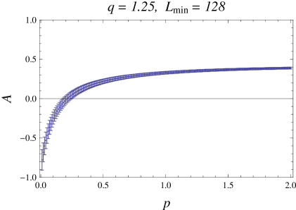
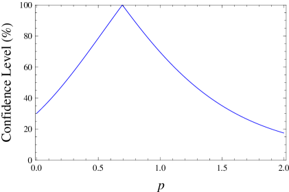
In Figure 5 we plot the results of our fits to as a function of , for and 32:
-
•
For an excellent confidence level is obtained over the whole range (and indeed beyond), with an optimum at (CL = 92%). The estimated amplitudes are positive and very far from zero; at the optimum we have . As the amplitude tends to a value , which is close to that obtained from the fit to .
-
•
For an excellent confidence level is again obtained over the whole range (and indeed beyond), with an optimum at (CL = 84%) but with a very broad peak. The estimated amplitudes are again positive and very far from zero; at the optimum we have . As the amplitude again tends to .
2) For the fit to is decent already for (, 2 DF, CL = 32%) and excellent for :
| (7.18) |
Once again this behavior is not surprising, because our fit to with free yielded with , which is not very far from .
In Figure 6 we plot the results of our fits to as a function of , for and 64:
-
•
For a decent confidence level is obtained for , with an optimum at (CL = 41%). The estimated amplitudes are positive and far from zero; at the optimum we have . As the amplitude tends to a value , which is close to that obtained from the fit to .
-
•
For a decent confidence level is obtained over the entire range (or even beyond), with an optimum at (CL = 96%). The estimated amplitudes are again positive and far from zero, and in fact quite close to those obtained from . At the optimum, we have .
3) For the fit to is poor even for (CL = 3%). In Figure 7 we plot the results of our fits to as a function of , for and 64:
-
•
For a decent confidence level is obtained for , but with the optimum attained at the ridiculously small value (CL = 86%). Also, the estimated amplitude is negative for , which is obviously impossible. However, for a decent fit is obtained with an amplitude that is positive and far from zero.
-
•
For a decent confidence level is obtained for , with an optimum at (CL = 86%). The estimated amplitudes are again negative for but positive and far from zero for . At the optimum, we have .
4) For the fit to is poor even for (CL = 1%). The fits to are poor (CL ) for and 64 for all . For , however, we are able to obtain decent fits over the whole range , as shown in Figure 8. The optimum lies at (CL = 99.9997%). The estimated amplitudes are negative for but positive and far from zero for . At the optimum, we have .
The foregoing fits show that the Ossola–Sokal conjecture is not ruled out by our data at . Indeed, our data are consistent with the possibility that exactly for , but with an amplitude that vanishes as , perhaps proportional to (the fits for and 1.50 are consistent with this latter behavior).
7.6 Dynamic critical exponents for other
Let us now look briefly at the dynamic critical exponents for observables other than . For , the values of are very close to those of , so the estimates of will be nearly the same; little would be gained by going through these fits in detail. Instead, it seems sensible to look at the observable that has the smallest autocorrelation time, namely — the idea being that if any differences in between different observables are to be detected, they will be detected here.
From Figure 3 we see that the autocorrelation function of is nearly a pure exponential (and this is so for all ), so that and hence or nearly so. The autocorrelation function of , by contrast, exhibits an initial fast decay, followed by a decay at the same exponential rate as for the other observables but with an amplitude that is significantly less than 1 (e.g. around 0.4 in the plot shown). The key question is whether this amplitude tends to a nonzero value when (in which case we will have ) or tends to zero as an inverse power of (in which case we will have ).181818 See [20, Section 5.2] for a more detailed analysis of this kind, for the Swendsen–Wang dynamics for the three-dimensional Ising model.
In Tables 26 and 27 we show the fits for to the ansätze and . In Table 28 we show the results for obtained by averaging over .
The estimates for are indeed less than those for , by an amount that is for and tends to zero as . The question is: Are these differences real, or are they artifacts of corrections to scaling at small ? The fact that the differences are smaller for , where the autocorrelation times are larger, suggests that perhaps the differences will disappear as but that at small we have to go to larger to see this. But this is far from clear; we will only know the truth by doing simulations at significantly larger values of .
8 Discussion
In this paper we have studied the dynamic critical behavior of the Chayes–Machta algorithm as a function of over the whole range . We have obtained estimates of the dynamic critical exponent as a function of : see (7.16), Table 24 and Figure 4. Since the autocorrelation function is nearly a pure exponential, we also expect that the dynamic critical exponent is either exactly equal or almost exactly equal to .
By simultaneously studying the whole range of values of , we were able to gain some insights that would not have been available had we studied only a single value of (such as the Ising value ) or even all integer values of as in past studies of the Swendsen–Wang algorithm. For instance:
1) The autocorrelation time at can be plausibly fit with the ansatz , suggesting that the Li–Sokal bound might be sharp modulo a logarithm; this agrees with the conclusions of the paper [16], where the data were in fact found to slightly favor the non-sharp-by-a-logarithm ansatz over the non-sharp-by-a-power ansatz. But we now find that the good fit to persists over the whole range . And it seems to us implausible on theoretical grounds that we would have such a logarithmic growth for an entire interval of ; rather, we expect that there exists one value such that for and for , with a possible (poly)logarithmic growth at . Our data suggest that lies between 1.25 and 1.75, with our best guess being around 1.6. If this scenario is correct, it follows that the Li–Sokal bound is non-sharp by a power for . This then suggests (but of course does not prove) that it might be non-sharp by a power over the whole interval (possibly reverting to non-sharp by a logarithm at ).
2) By considering the Ossola–Sokal conjecture simultaneously for all , we can see immediately that it fails at (where but ) and hence fails also for near 1 if the dynamic critical exponent is a continuous function of . Indeed, our pure power-law fits suggest that the conjecture fails for . (In particular, if as just suggested, then the conjecture fails spectacularly in the interval , where but .) However — and perhaps surprisingly — our data are also compatible with an alternative scenario in which exactly for all near 1, but with an amplitude that vanishes as (Section 7.5).
However, the behavior of the Chayes–Machta autocorrelation time for is still unclear: though our data strongly suggest that diverges as for slightly below 2, and is nondivergent as for slightly above 1, we cannot rule out the possibility that the data at are misleading and that the true asymptotic behavior is different from what we conjecture. Future work at larger values of would of course be desirable.
Likewise, though our data suggest that the Li–Sokal bound is non-sharp by a power for , it is also true that the exponent estimates have been dropping over time as data becomes available at larger values of and as we try ansätze other than a pure power law (see Table 24 for the effect of the ansatz). Our data suggest most clearly the non-sharpness of the Li–Sokal bound (when the non-sharpness is measured in units of the standard deviation of our estimate) at and . At these values of , the critical slowing-down is strong enough that interference from the regular background term is less important than it is at smaller (i.e. the and fits show less discrepancy) but modest enough that we can have reasonably good data on large lattices (contrary to the situation at larger ); furthermore, the correction-to-scaling exponent is still fairly large. It would therefore be of great interest to perform high-precision simulations at these values of , going to very high values of .
Acknowledgments
The authors would like to thank Youjin Deng and Jonathan Machta for many helpful discussions. We would also like to thank Mulin Ding for helping us to recover some of the data from this project.
This research was supported in part by U.S. National Science Foundation grants PHY–0116590 and PHY–0424082.
References
- [1] K. Binder, ed., Monte Carlo Methods in Statistical Physics, 2nd ed. (Springer-Verlag, Berlin, 1986).
- [2] K. Binder, ed., Applications of the Monte Carlo Method in Statistical Physics, 2nd ed. (Springer-Verlag, Berlin, 1987).
- [3] K. Binder, ed., The Monte Carlo Method in Condensed Matter Physics, 2nd ed. (Springer-Verlag, Berlin, 1995).
- [4] P.C. Hohenberg and B.I. Halperin, Rev. Mod. Phys. 49, 435 (1977).
- [5] A. D. Sokal, Monte Carlo methods in Statistical Mechanics: Foundations and new algorithms, in C. DeWitt-Morette, P. Cartier and A. Folacci, eds., Functional Integration: Basics and Applications (1996 Cargèse summer school), pp. 131–192 (Plenum, New York, 1997).
- [6] R. H. Swendsen and J.-S. Wang, Phys. Rev. Lett. 58, 86 (1987).
- [7] R. B. Potts, Proc. Cambridge Philos. Soc. 48, 106 (1952).
- [8] F. Y. Wu, Rev. Mod. Phys. 54, 235 (1982) and erratum 55, 315 (1983).
- [9] F. Y. Wu, J. Appl. Phys. 55, 2421 (1984).
- [10] P. W. Kasteleyn and C. M. Fortuin, J. Phys. Soc. Japan 26 (Suppl.), 11 (1969).
- [11] C. M. Fortuin and P. W. Kasteleyn, Physica 57, 536 (1972).
- [12] C. M. Fortuin, Physica 58, 393 (1972).
- [13] C. M. Fortuin, Physica 59, 545 (1972).
- [14] R.G. Edwards and A.D. Sokal, Phys. Rev. D 38, 2009 (1988).
- [15] G. Grimmett, The Random-Cluster Model (Springer-Verlag, New York, 2006).
- [16] J. Salas and A.D. Sokal, Universal amplitude ratios in the critical two-dimensional Ising model on a torus, cond-mat/9904038v1. For space reasons, this material was deleted from the published version of this paper [J. Stat. Phys. 98, 551 (2000)].
- [17] J. Salas and A.D. Sokal, J. Stat. Phys. 87, 1 (1997), hep-lat/9605018.
- [18] J. Salas and A.D. Sokal, J. Stat. Phys. 85, 297 (1996), hep-lat/9511022.
- [19] J. Salas and A.D. Sokal, J. Stat. Phys. 88, 567 (1997), hep-lat/9607030.
- [20] G. Ossola and A.D. Sokal, Nucl. Phys. B 691, 259 (2004), hep-lat/0402019.
- [21] W. Klein, T. Ray and P. Tamayo, Phys. Rev. Lett. 62, 163 (1989).
- [22] T. Ray, P. Tamayo and W. Klein, Phys. Rev. A 39, 5949 (1989).
- [23] P.D. Coddington and C.F. Baillie, Phys. Rev. Lett. 68, 962 (1992).
- [24] N. Persky, R. Ben-Av, I. Kanter and E. Domany, Phys. Rev. E 54, 2351 (1996), cond-mat/9603134.
- [25] L. Chayes and J. Machta, Physica A 254, 477 (1998).
- [26] H.W.J. Blöte, Y. Deng, X. Qian and A.D. Sokal, in preparation,
- [27] Y. Deng, T. M. Garoni and A. D. Sokal, Dynamic critical behavior of the Chayes-Machta algorithm for the random-cluster model, II. Three dimensions, in preparation.
- [28] Y. Deng, T. M. Garoni, J. Machta and A. D. Sokal, Dynamic critical behavior of the Chayes-Machta algorithm for the random-cluster model, III. Complete graph, in preparation.
- [29] Y. Deng, T. M. Garoni, J. Machta, G. Ossola, M. Polin and A. D. Sokal, Phys. Rev. Lett. 99, 055701 (2007), arXiv:0705.2751 [cond-mat.stat-mech].
- [30] R. J. Baxter, Exactly Solved Models in Statistical Mechanics (Academic Press, London–New York, 1982).
- [31] V. Beffara and H. Duminil-Copin, The self-dual point of the two-dimensional random-cluster model is critical for , arXiv:1006.5073 [math.PR].
- [32] B. Nienhuis, J. Stat. Phys. 34, 731 (1984).
- [33] B. Nienhuis, in Phase Transitions and Critical Phenomena, vol. 11, C. Domb and J.L. Lebowitz, eds. (Academic Press, New York–London, 1987), section IV.C.
- [34] M.P.M. den Nijs, Phys. Rev. B 27, 1674 (1983).
- [35] X.-J. Li and A. D. Sokal, Phys. Rev. Lett. 63, 827 (1989).
- [36] D. J. Amit and V. Martín-Mayor, Field Theory, the Renormalization Group, and Critical Phenomena, 3rd ed. (World Scientific, Singapore, 2005).
- [37] S. Caracciolo, R. G. Edwards, A. Pelissetto and A. D. Sokal, Nucl. Phys. B 403, 475 (1993), hep-lat/9205005.
- [38] F. Cooper, B. Freedman and D. Preston, Nucl. Phys. B 210 [FS6], 210 (1982).
- [39] M. B. Priestley, Spectral Analysis and Time Series, 2 vols. (Academic, London, 1981).
- [40] T. W. Anderson, The Statistical Analysis of Time Series (Wiley, New York, 1971).
- [41] N. Madras and A. D. Sokal, J. Stat. Phys. 50, 109 (1988).
- [42] G. Ossola and A.D. Sokal, Phys. Rev. E 70, 027701 (2004), hep-lat/0403010.
- [43] P. L’Ecuyer, Math. Comp. 68, 249 (1999).
- [44] H. Guo and D. Jasnow, Phys. Rev. B 35, 1846 (1987); 39, 753 (E) (1989).
- [45] X. Feng, Y. Deng and H.W.J. Blöte, Phys. Rev. E 78, 031136 (2008), arXiv:0901.1370 [cond-mat.stat-mech].
- [46] H.W.J. Blöte and M.P.M. den Nijs, Phys. Rev. B 37, 1766 (1988).
- [47] P. Di Francesco, H. Saleur and J.-B. Zuber, Nucl. Phys. B 290 [FS20], 527 (1987).
- [48] P. Di Francesco, H. Saleur and J.-B. Zuber, Europhys. Lett. 5, 95 (1988).
- [49] J. Salas and A.D. Sokal, J. Stat. Phys. 98, 551 (2000), cond-mat/9904038.
- [50] A.E. Ferdinand and M.E. Fisher, Phys. Rev. 185, 832 (1969).
- [51] J. Salas, J. Phys. A 34, 1311 (2001), cond-mat/0009054.
| 1.25 | 0.35527 | 0.11118 | 1.77764 | 1.80702 |
|---|---|---|---|---|
| 1.50 | 0.22663 | 0.11678 | 1.76644 | 1.63551 |
| 1.75 | 0.10929 | 0.12131 | 1.75738 | 1.47905 |
| 2.00 | 0.00000 | 0.12500 | 1.75000 | 1.33333 |
| 2.25 | 0.10363 | 0.12798 | 1.74404 | 1.19517 |
| 2.50 | 0.20357 | 0.13034 | 1.73932 | 1.06191 |
| 2.75 | 0.30168 | 0.13212 | 1.73576 | 0.93110 |
| 3.00 | 0.40000 | 0.13333 | 1.73333 | 0.80000 |
| 3.25 | 0.50126 | 0.13393 | 1.73214 | 0.66499 |
| 3.50 | 0.61007 | 0.13377 | 1.73246 | 0.51991 |
| 3.75 | 0.73760 | 0.13242 | 1.73517 | 0.34986 |
| 4.00 | 1.00000 | 0.12500 | 1.75000 | 0.00000 |
| 16 | (38) | (59) | (83) | (68) | ||||
| 32 | (20) | (32) | (47) | (41) | ||||
| 64 | (10) | (17) | (26) | (24) | ||||
| 128 | (5) | (9) | (14) | (14) | ||||
| 256 | (3) | (5) | (8) | (8) | ||||
| 512 | (2) | (3) | (6) | (6) | ||||
| 1024 | (2) | (3) | (5) | (6) | ||||
| 16 | (91) | (117) | (149) | (136) | ||||
| 32 | (56) | (76) | (101) | (97) | ||||
| 64 | (34) | (49) | (68) | (68) | ||||
| 128 | (21) | (31) | (45) | (47) | ||||
| 256 | (12) | (19) | (29) | (33) | ||||
| 512 | (10) | (17) | (26) | (32) | ||||
| 1024 | (10) | (17) | (28) | (35) | ||||
| 16 | (167) | (202) | (243) | (230) | ||||
| 32 | (124) | (157) | (197) | (196) | ||||
| 64 | (92) | (122) | (162) | (169) | ||||
| 128 | (67) | (95) | (133) | (148) | ||||
| 256 | (49) | (74) | (111) | (132) | ||||
| 512 | (51) | (82) | (128) | (170) | ||||
| 1024 | (59) | (100) | (173) | (242) | ||||
| 16 | ||||||||
| 32 | ||||||||
| 64 | ||||||||
| 128 | ||||||||
| 256 | ||||||||
| 512 | ||||||||
| 1024 | ||||||||
| 16 | ||||||||
| 32 | ||||||||
| 64 | ||||||||
| 128 | ||||||||
| 256 | ||||||||
| 512 | ||||||||
| 1024 | ||||||||
| 16 | ||||||||
| 32 | ||||||||
| 64 | ||||||||
| 128 | ||||||||
| 256 | ||||||||
| 512 | ||||||||
| 1024 | ||||||||
| 16 | ||||||||
| 32 | ||||||||
| 64 | ||||||||
| 128 | ||||||||
| 256 | ||||||||
| 512 | ||||||||
| 1024 | ||||||||
| 16 | ||||||||
| 32 | ||||||||
| 64 | ||||||||
| 128 | ||||||||
| 256 | ||||||||
| 512 | ||||||||
| 1024 | ||||||||
| 16 | ||||||||
| 32 | ||||||||
| 64 | ||||||||
| 128 | ||||||||
| 256 | ||||||||
| 512 | ||||||||
| 1024 | ||||||||
| 16 | (10) | (13) | (17) | (13) | ||||
| 32 | (10) | (13) | (17) | (13) | ||||
| 64 | (10) | (14) | (18) | (14) | ||||
| 128 | (10) | (14) | (19) | (15) | ||||
| 256 | (10) | (14) | (20) | (16) | ||||
| 512 | (14) | (20) | (27) | (24) | ||||
| 1024 | (23) | (33) | (46) | (40) | ||||
| 16 | (16) | (19) | (22) | (20) | ||||
| 32 | (17) | (21) | (26) | (23) | ||||
| 64 | (18) | (23) | (29) | (27) | ||||
| 128 | (20) | (26) | (33) | (32) | ||||
| 256 | (21) | (29) | (38) | (37) | ||||
| 512 | (32) | (45) | (57) | (61) | ||||
| 1024 | (56) | (78) | (109) | (114) | ||||
| 16 | (23) | (27) | (31) | (29) | ||||
| 32 | (28) | (33) | (40) | (38) | ||||
| 64 | (33) | (41) | (51) | (50) | ||||
| 128 | (40) | (52) | (66) | (67) | ||||
| 256 | (49) | (65) | (86) | (92) | ||||
| 512 | (84) | (115) | (155) | (178) | ||||
| 1024 | (160) | (229) | (329) | (386) | ||||
| 16 | ||||||||
| 32 | ||||||||
| 64 | ||||||||
| 128 | ||||||||
| 256 | ||||||||
| 512 | ||||||||
| 1024 | ||||||||
| 16 | ||||||||
| 32 | ||||||||
| 64 | ||||||||
| 128 | ||||||||
| 256 | ||||||||
| 512 | ||||||||
| 1024 | ||||||||
| 16 | ||||||||
| 32 | ||||||||
| 64 | ||||||||
| 128 | ||||||||
| 256 | ||||||||
| 512 | ||||||||
| 1024 | ||||||||
| 16 | ||||||||
| 32 | ||||||||
| 64 | ||||||||
| 128 | ||||||||
| 256 | ||||||||
| 512 | ||||||||
| 1024 | ||||||||
| 16 | ||||||||
| 32 | ||||||||
| 64 | ||||||||
| 128 | ||||||||
| 256 | ||||||||
| 512 | ||||||||
| 1024 | ||||||||
| 16 | ||||||||
| 32 | ||||||||
| 64 | ||||||||
| 128 | ||||||||
| 256 | ||||||||
| 512 | ||||||||
| 1024 | ||||||||
| 16 | ||||||||
| 32 | ||||||||
| 64 | ||||||||
| 128 | ||||||||
| 256 | ||||||||
| 512 | ||||||||
| 1024 | ||||||||
| 16 | ||||||||
| 32 | ||||||||
| 64 | ||||||||
| 128 | ||||||||
| 256 | ||||||||
| 512 | ||||||||
| 1024 | ||||||||
| 16 | ||||||||
| 32 | ||||||||
| 64 | ||||||||
| 128 | ||||||||
| 256 | ||||||||
| 512 | ||||||||
| 1024 | ||||||||
| 16 | ||||||||
| 32 | ||||||||
| 64 | ||||||||
| 128 | ||||||||
| 256 | ||||||||
| 512 | ||||||||
| 1024 | ||||||||
| 16 | ||||||||
| 32 | ||||||||
| 64 | ||||||||
| 128 | ||||||||
| 256 | ||||||||
| 512 | ||||||||
| 1024 | ||||||||
| 16 | ||||||||
| 32 | ||||||||
| 64 | ||||||||
| 128 | ||||||||
| 256 | ||||||||
| 512 | ||||||||
| 1024 | ||||||||
| 16 | ||||||||
| 32 | ||||||||
| 64 | ||||||||
| 128 | ||||||||
| 256 | ||||||||
| 512 | ||||||||
| 1024 | ||||||||
| 16 | ||||||||
| 32 | ||||||||
| 64 | ||||||||
| 128 | ||||||||
| 256 | ||||||||
| 512 | ||||||||
| 1024 | ||||||||
| 16 | ||||||||
| 32 | ||||||||
| 64 | ||||||||
| 128 | ||||||||
| 256 | ||||||||
| 512 | ||||||||
| 1024 | ||||||||
| 16 | ||||||||
| 32 | ||||||||
| 64 | ||||||||
| 128 | ||||||||
| 256 | ||||||||
| 512 | ||||||||
| 1024 | ||||||||
| 16 | ||||||||
| 32 | ||||||||
| 64 | ||||||||
| 128 | ||||||||
| 256 | ||||||||
| 512 | ||||||||
| 1024 | ||||||||
| 16 | ||||||||
| 32 | ||||||||
| 64 | ||||||||
| 128 | ||||||||
| 256 | ||||||||
| 512 | ||||||||
| 1024 | ||||||||
| 16 | ||||||||
| 32 | ||||||||
| 64 | ||||||||
| 128 | ||||||||
| 256 | ||||||||
| 512 | ||||||||
| 1024 | ||||||||
| 16 | ||||||||
| 32 | ||||||||
| 64 | ||||||||
| 128 | ||||||||
| 256 | ||||||||
| 512 | ||||||||
| 1024 | ||||||||
| 16 | ||||||||
| 32 | ||||||||
| 64 | ||||||||
| 128 | ||||||||
| 256 | ||||||||
| 512 | ||||||||
| 1024 | ||||||||
| 16 | ||||||||
| 32 | ||||||||
| 64 | ||||||||
| 128 | ||||||||
| 256 | ||||||||
| 512 | ||||||||
| 1024 | ||||||||
| 16 | ||||||||
| 32 | ||||||||
| 64 | ||||||||
| 128 | ||||||||
| 256 | ||||||||
| 512 | ||||||||
| 1024 | ||||||||
| 16 | ||||||||
| 32 | ||||||||
| 64 | ||||||||
| 128 | ||||||||
| 256 | ||||||||
| 512 | ||||||||
| 1024 | ||||||||
| Fits to | Fits to | ||||||||||||
|---|---|---|---|---|---|---|---|---|---|---|---|---|---|
| DF | CL(%) | DF | CL(%) | (exact) | |||||||||
| 1.25 | 256 | 0.91734(8) | 1.48 | 2 | 48 | 16 | 0.91735(7) | 0.900(243) | 1.81(10) | 2.53 | 4 | 64 | 1.80702 |
| 1.50 | 128 | 0.90867(9) | 0.17 | 3 | 98 | 16 | 0.90857(10) | 0.563(173) | 1.62(11) | 0.77 | 4 | 94 | 1.63551 |
| 1.75 | 128 | 0.90496(12) | 5.19 | 3 | 16 | 16 | 0.90487(14) | 0.582(228) | 1.62(14) | 6.93 | 4 | 14 | 1.47905 |
| 2.00 | 512 | 0.90442(20) | 0.54 | 1 | 46 | 32 | 0.90387(74) | 0.017(9) | 0.49(21) | 4.12 | 3 | 25 | 1.33333 |
| 2.25 | 256 | 0.90786(17) | 1.30 | 2 | 52 | [16] | 0.90799(16) | 0.465(184) | 1.55(15) | 8.19 | 4 | 8 | 1.19517 |
| 2.50 | 64 | 0.91369(14) | 3.36 | 4 | 50 | 16 | 0.91335(21) | 0.396(195) | 1.50(18) | 3.69 | 4 | 45 | 1.06191 |
| 2.75 | 256 | 0.92092(30) | 0.06 | 2 | 97 | 16 | 0.92085(45) | 0.066(33) | 0.92(20) | 5.96 | 4 | 20 | 0.93110 |
| 3.00 | 64 | 0.93193(17) | 0.13 | 4 | 100 | 16 | 0.93184(23) | 0.704(1.120) | 1.97(59) | 0.02 | 4 | 100 | 0.80000 |
| 3.25 | 128 | 0.94503(29) | 0.97 | 3 | 81 | — | — | — | — | — | — | — | 0.66499 |
| 3.50 | 256 | 0.96069(55) | 0.30 | 2 | 86 | 16 | 0.96223(198) | 0.025(9) | 0.47(23) | 1.21 | 4 | 88 | 0.51991 |
| 3.75 | 256 | 0.98051(73) | 0.03 | 2 | 99 | 32 | 0.98591(540) | 0.060(27) | 0.41(23) | 1.19 | 3 | 75 | 0.34986 |
| 4.00 | 256 | 1.00434(80) | 0.84 | 2 | 66 | 16 | 1.01323(335) | 0.100(9) | 0.41(7) | 4.81 | 4 | 31 | 0.00000 |
| Fits to | |||||||||
|---|---|---|---|---|---|---|---|---|---|
| DF | CL(%) | (exact) | deviation | dev() | |||||
| 1.25 | 256 | 1.77773(9) | 1.0496(6) | 1.40 | 1 | 24 | 1.77764 | 0.00009 | 1.0 |
| 1.50 | 128 | 1.76639(8) | 1.0645(5) | 0.30 | 2 | 86 | 1.76644 | 0.00005 | 0.6 |
| 1.75 | 128 | 1.75759(12) | 1.0768(7) | 2.34 | 2 | 31 | 1.75738 | 0.00022 | 1.8 |
| 2.00 | 128 | 1.74969(11) | 1.0937(6) | 2.54 | 2 | 28 | 1.75000 | 0.00031 | 2.9 |
| 2.25 | 256 | 1.74428(26) | 1.1039(17) | 1.37 | 1 | 24 | 1.74404 | 0.00024 | 0.9 |
| 2.50 | 256 | 1.73902(37) | 1.1209(24) | 0.01 | 1 | 94 | 1.73932 | 0.00030 | 0.8 |
| 2.75 | 128 | 1.73575(28) | 1.1316(17) | 0.85 | 2 | 65 | 1.73576 | 0.00001 | 0.03 |
| 3.00 | 128 | 1.73438(28) | 1.1371(17) | 0.72 | 2 | 70 | 1.73333 | 0.00105 | 3.8 |
| 3.25 | 128 | 1.73341(37) | 1.1460(23) | 0.30 | 2 | 86 | 1.73214 | 0.00127 | 3.4 |
| 3.50 | 256 | 1.73304(99) | 1.1571(67) | 0.01 | 1 | 93 | 1.73246 | 0.00058 | 0.6 |
| 3.75 | 128 | 1.73745(67) | 1.1431(40) | 1.46 | 2 | 48 | 1.73517 | 0.00229 | 3.4 |
| 4.00 | 256 | 1.73968(152) | 1.1502(101) | 0.44 | 1 | 51 | 1.75000 | 0.01032 | 6.8 |
| Fits to | Fits to | ||||||||||||
|---|---|---|---|---|---|---|---|---|---|---|---|---|---|
| DF | CL(%) | DF | CL(%) | (exact) | |||||||||
| 1.25 | 256 | 1.05017(5) | 2.38 | 2 | 30 | 16 | 1.05013(8) | 0.011(5) | 0.87(19) | 4.72 | 4 | 32 | 1.80702 |
| 1.50 | 128 | 1.06417(6) | 0.70 | 3 | 87 | 16 | 1.06379(53) | 0.003(1) | 0.34(30) | 1.55 | 4 | 82 | 1.63551 |
| 1.75 | 64 | 1.07811(7) | 7.16 | 4 | 13 | — | — | — | — | — | — | — | 1.47905 |
| 2.00 | 512 | 1.09148(15) | 0.50 | 1 | 48 | [16] | 1.09195(8) | 0.231(316) | 1.88(50) | 15.63 | 4 | 0.4 | 1.33333 |
| 2.25 | 256 | 1.10545(13) | 2.19 | 2 | 33 | [16] | 1.10565(15) | 0.078(43) | 1.22(21) | 7.84 | 4 | 10 | 1.19517 |
| 2.50 | 128 | 1.11875(14) | 2.34 | 3 | 51 | 16 | 1.11912(26) | 0.062(22) | 0.94(14) | 3.96 | 4 | 41 | 1.06191 |
| 2.75 | 128 | 1.13159(18) | 0.85 | 3 | 84 | 16 | 1.13192(29) | 0.161(51) | 1.12(12) | 5.80 | 4 | 21 | 0.93110 |
| 3.00 | 256 | 1.14415(25) | 1.71 | 2 | 43 | 16 | 1.14541(49) | 0.086(12) | 0.73(6) | 0.43 | 4 | 98 | 0.80000 |
| 3.25 | 512 | 1.15559(63) | 0.25 | 1 | 62 | 16 | 1.15656(67) | 0.111(14) | 0.70(6) | 2.74 | 4 | 60 | 0.66499 |
| 3.50 | 256 | 1.16102(46) | 0.35 | 2 | 84 | 16 | 1.16365(96) | 0.119(15) | 0.65(6) | 0.99 | 4 | 91 | 0.51991 |
| 3.75 | 256 | 1.15852(61) | 0.42 | 2 | 81 | 16 | 1.16358(199) | 0.080(9) | 0.48(7) | 0.79 | 4 | 94 | 0.34986 |
| 4.00 | [512] | 1.07693(124) | 2.97 | 1 | 8 | — | — | — | — | — | — | — | 0.00000 |
| Fits to | |||||||||
|---|---|---|---|---|---|---|---|---|---|
| DF | CL(%) | (exact) | deviation | dev() | |||||
| 1.25 | 256 | 0.11111(6) | 0.9896(3) | 1.29 | 1 | 26 | 0.11118 | 0.00007 | 1.2 |
| 1.50 | 16 | 0.11681(2) | 0.9958(1) | 2.01 | 5 | 85 | 0.11678 | 0.00003 | 1.6 |
| 1.75 | 128 | 0.12115(8) | 1.0004(4) | 2.21 | 2 | 33 | 0.12131 | 0.00016 | 2.1 |
| 2.00 | 128 | 0.12518(7) | 1.0080(4) | 2.04 | 2 | 36 | 0.12500 | 0.00018 | 2.7 |
| 2.25 | 256 | 0.12787(17) | 1.0118(10) | 1.20 | 1 | 27 | 0.12798 | 0.00011 | 0.6 |
| 2.50 | 128 | 0.13033(13) | 1.0177(7) | 1.48 | 2 | 48 | 0.13034 | 0.00001 | 0.10 |
| 2.75 | 128 | 0.13230(18) | 1.0237(10) | 1.65 | 2 | 44 | 0.13212 | 0.00018 | 1.0 |
| 3.00 | 64 | 0.13283(11) | 1.0245(5) | 1.24 | 3 | 74 | 0.13333 | 0.00050 | 4.6 |
| 3.25 | 128 | 0.13366(24) | 1.0295(13) | 0.86 | 2 | 65 | 0.13393 | 0.00027 | 1.1 |
| 3.50 | 64 | 0.13315(19) | 1.0289(9) | 2.39 | 3 | 50 | 0.13377 | 0.00062 | 3.3 |
| 3.75 | 32 | 0.13174(15) | 1.0263(7) | 1.74 | 4 | 78 | 0.13242 | 0.00067 | 4.4 |
| 4.00 | 256 | 0.13200(104) | 1.0357(62) | 0.54 | 1 | 46 | 0.12500 | 0.00700 | 6.8 |
| Fits to | Fits to | |||||||||||||||
|---|---|---|---|---|---|---|---|---|---|---|---|---|---|---|---|---|
| DF | CL(%) | DF | CL(%) | (exact) | dev | dev() | ||||||||||
| 1.25 | [256] | 0.0406(9) | 0.588(3) | 16.40 | 1 | 16 | 0.3675(49) | 0.791(6) | 0.839(2) | 1.82 | 4 | 77 | 0.35527 | 0.012 | 2.5 | |
| 1.50 | [256] | 0.0712(8) | 1.036(5) | 30.87 | 1 | 128 | 0.1977(186) | 1.933(23) | 2.182(59) | 0.37 | 1 | 54 | 0.22663 | 0.029 | 1.6 | |
| 1.75 | [256] | 0.1089(8) | 1.366(7) | 31.62 | 1 | 128 | 0.0965(135) | 5.413(347) | 5.665(440) | 0.15 | 1 | 70 | 0.10929 | 0.013 | 0.9 | |
| 2.00 | [256] | 0.1569(6) | 1.554(6) | 43.28 | 1 | (see text) | — | — | — | — | — | — | 0() | — | — | |
| 2.25 | [256] | 0.2143(8) | 1.608(8) | 36.65 | 1 | 128 | 0.1108(65) | 5.856(558) | 5.554(640) | 0.45 | 1 | 50 | 0.10363 | 0.007 | 1.1 | |
| 2.50 | [256] | 0.2778(10) | 1.573(10) | 9.47 | 1 | 0.2 | 64 | 0.2025(32) | 3.421(109) | 3.176(150) | 0.73 | 2 | 69 | 0.20357 | 0.001 | 0.3 |
| 2.75 | [256] | 0.3488(13) | 1.457(11) | 7.44 | 1 | 0.6 | 32 | 0.2995(18) | 2.293(33) | 2.001(54) | 0.39 | 3 | 94 | 0.30168 | 0.002 | 1.2 |
| 3.00 | 256 | 0.4254(13) | 1.295(10) | 0.42 | 1 | 52 | 32 | 0.3947(15) | 1.681(18) | 1.296(37) | 2.14 | 3 | 54 | 0.40000 | 0.005 | 3.6 |
| 3.25 | [256] | 0.5063(17) | 1.120(11) | 2.94 | 1 | 9 | 32 | 0.4902(16) | 1.275(14) | 0.771(38) | 3.04 | 3 | 39 | 0.50126 | 0.011 | 6.8 |
| 3.50 | 64 | 0.5952(7) | 0.921(3) | 0.94 | 3 | 82 | 64 | 0.5945(35) | 0.925(22) | 0.020(102) | 0.90 | 2 | 64 | 0.61007 | 0.016 | 4.5 |
| 3.75 | 256 | 0.6920(31) | 0.724(13) | 0.69 | 1 | 41 | 128 | 0.7095(86) | 0.635(38) | 1.149(369) | 0.03 | 1 | 86 | 0.73760 | 0.028 | 3.3 |
| 4.00 | 256 | 0.7998(35) | 0.534(11) | 0.35 | 1 | 55 | 128 | 0.8338(85) | 0.416(24) | 2.713(392) | 0.53 | 1 | 47 | 1 () | 0.166 | 19.6 |
| 16 | 2.143(3) | 2.020(7) |
|---|---|---|
| 32 | 2.123(4) | 2.013(9) |
| 64 | 2.100(4) | 1.990(11) |
| 128 | 2.080(4) | 2.015(14) |
| 256 | 2.069(5) | 1.991(17) |
| 512 | 2.047(7) | 2.034(30) |
| 1024 | 2.051(12) | 1.953(56) |
| Fits to | ||||||
| DF | CL(%) | |||||
| 2.00 | 2 | 512 | 2.048(6) | 0.09 | 1 | 76 |
| 2.25 | 2 | 256 | 2.036(5) | 0.51 | 2 | 77 |
| 2.50 | 2 | 128 | 2.022(5) | 0.02 | 3 | 100 |
| 2.75 | 2 | 128 | 2.006(6) | 0.87 | 3 | 83 |
| 3.00 | 2 | 32 | 2.015(5) | 3.63 | 5 | 60 |
| 3.25 | 2 | 32 | 2.005(6) | 5.40 | 5 | 37 |
| 3.50 | 2 | 16 | 2.015(5) | 6.74 | 6 | 35 |
| 3.75 | 2 | 16 | 2.014(6) | 1.68 | 6 | 95 |
| 4.00 | 2 | 16 | 2.011(7) | 2.75 | 6 | 84 |
| 3.00 | 3 | 256 | 3.011(16) | 0.66 | 2 | 72 |
| 3.25 | 3 | 64 | 3.012(11) | 3.18 | 4 | 53 |
| 3.50 | 3 | 64 | 3.014(13) | 3.67 | 4 | 45 |
| 3.75 | 3 | 16 | 3.034(9) | 2.32 | 6 | 89 |
| 4.00 | 3 | 64 | 2.988(19) | 1.66 | 4 | 80 |
| 4.00 | 4 | 64 | 4.002(25) | 3.01 | 4 | 56 |
| Fits to | |||||||
| DF | CL(%) | ||||||
| 1.25 | 1 | [256] | 0.053(1) | 1.27(1) | 3.76 | 1 | 5 |
| 1.50 | 1 | [256] | 0.104(2) | 2.20(2) | 3.84 | 1 | 5 |
| 1.75 | 1 | 256 | 0.158(2) | 3.28(5) | 0.21 | 1 | 65 |
| 2.00 | 1 | 256 | 0.215(3) | 4.47(9) | 0.06 | 1 | 81 |
| 2.00 | 2 | [256] | 0.224(2) | 2.06(3) | 6.91 | 1 | 0.9 |
| 2.25 | 1 | 256 | 0.286(4) | 5.35(14) | 2.16 | 1 | 14 |
| 2.25 | 2 | [256] | 0.287(3) | 2.62(5) | 10.68 | 1 | 0.1 |
| 2.50 | 1 | 256 | 0.353(6) | 6.35(23) | 0.02 | 1 | 90 |
| 2.50 | 2 | 256 | 0.353(4) | 3.15(8) | 0.06 | 1 | 80 |
| 2.75 | 1 | 256 | 0.424(8) | 7.19(34) | 0.07 | 1 | 80 |
| 2.75 | 2 | [256] | 0.421(5) | 3.66(12) | 3.02 | 1 | 8 |
| 3.00 | 1 | 128 | 0.505(6) | 7.52(23) | 1.18 | 2 | 56 |
| 3.00 | 2 | 128 | 0.516(4) | 3.55(8) | 1.46 | 2 | 48 |
| 3.00 | 3 | 256 | 0.505(6) | 2.51(9) | 0.04 | 1 | 84 |
| 3.25 | 1 | 128 | 0.590(7) | 7.66(30) | 3.14 | 2 | 21 |
| 3.25 | 2 | 256 | 0.585(10) | 3.96(23) | 0.003 | 1 | 96 |
| 3.25 | 3 | 256 | 0.585(8) | 2.64(13) | 0.02 | 1 | 90 |
| 3.50 | 1 | 128 | 0.676(10) | 7.77(39) | 1.07 | 2 | 58 |
| 3.50 | 2 | 16 | 0.693(2) | 3.54(2) | 2.39 | 5 | 79 |
| 3.50 | 3 | 64 | 0.695(3) | 2.33(4) | 0.05 | 3 | 100 |
| 3.75 | 1 | 32 | 0.779(4) | 7.14(13) | 0.94 | 4 | 92 |
| 3.75 | 2 | 32 | 0.784(3) | 3.46(4) | 1.63 | 4 | 80 |
| 3.75 | 3 | 128 | 0.798(7) | 2.14(8) | 0.70 | 2 | 71 |
| 4.00 | 1 | 128 | 0.916(16) | 5.44(46) | 0.15 | 2 | 93 |
| 4.00 | 2 | 128 | 0.909(12) | 2.84(17) | 0.75 | 2 | 69 |
| 4.00 | 3 | 64 | 0.890(5) | 2.09(5) | 1.58 | 3 | 66 |
| 4.00 | 4 | 256 | 0.938(17) | 1.18(12) | 0.06 | 1 | 81 |
| Fits to | ||||||||
| DF | CL(%) | |||||||
| 1.25 | 1 | 128 | 0.213(35) | 1.61(5) | 2.19(8) | 0.49 | 1 | 48 |
| 1.50 | 1 | 32 | 0.034(7) | 15.86(2.92) | 17.09(2.96) | 0.82 | 3 | 85 |
| 1.75 | 1 | 128 | 0.085(26) | 9.66(4.42) | 7.56(4.82) | 0.33 | 1 | 57 |
| 2.00 | 1 | 16 | 0.145(4) | 10.37(51) | 8.44(57) | 2.32 | 4 | 68 |
| 2.00 | 2 | 32 | 0.141(5) | 5.48(32) | 4.83(36) | 1.32 | 3 | 72 |
| 2.25 | 1 | 32 | 0.235(8) | 8.92(61) | 6.68(86) | 1.62 | 3 | 65 |
| 2.25 | 2 | [128] | 0.200(19) | 6.37(1.31) | 6.45(1.89) | 3.44 | 1 | 6 |
| 2.50 | 1 | 32 | 0.315(8) | 9.01(59) | 6.75(1.00) | 0.21 | 3 | 98 |
| 2.50 | 2 | 64 | 0.294(11) | 5.38(48) | 5.23(85) | 0.91 | 2 | 63 |
| 2.75 | 1 | 16 | 0.411(5) | 8.19(30) | 4.76(57) | 1.06 | 4 | 90 |
| 2.75 | 2 | 128 | 0.348(24) | 6.87(1.40) | 9.62(3.28) | 0.47 | 1 | 49 |
| 3.00 | 1 | 32 | 0.481(10) | 9.08(63) | 6.79(1.68) | 0.84 | 3 | 84 |
| 3.00 | 2 | 16 | 0.500(4) | 4.00(11) | 2.15(25) | 1.35 | 4 | 85 |
| 3.00 | 3 | 16 | 0.497(3) | 2.72(6) | 1.71(13) | 2.40 | 4 | 66 |
| 3.25 | 1 | 64 | 0.558(21) | 9.75(1.44) | 11.92(5.96) | 2.93 | 2 | 23 |
| 3.25 | 2 | 32 | 0.577(8) | 4.24(22) | 2.93(78) | 0.71 | 3 | 87 |
| 3.25 | 3 | 64 | 0.565(12) | 3.10(26) | 3.51(1.12) | 0.22 | 2 | 90 |
| 3.50 | 1 | 64 | 0.648(25) | 9.50(1.56) | 14.38(8.87) | 1.15 | 2 | 56 |
| 3.50 | 2 | 16 | 0.691(6) | 3.57(11) | 0.13(40) | 2.27 | 4 | 69 |
| 3.50 | 3 | 32 | 0.689(8) | 2.42(11) | 0.66(55) | 0.34 | 3 | 95 |
| 3.75 | 1 | 16 | 0.790(9) | 6.69(32) | 2.96(1.49) | 0.33 | 4 | 99 |
| 3.75 | 2 | 16 | 0.800(6) | 3.15(10) | 2.21(50) | 1.62 | 4 | 81 |
| 3.75 | 3 | 16 | 0.795(5) | 2.15(6) | 1.10(28) | 2.91 | 4 | 57 |
| 4.00 | 1 | 32 | 0.935(18) | 4.76(48) | 20.52(5.09) | 0.66 | 3 | 88 |
| 4.00 | 2 | 32 | 0.925(13) | 2.54(18) | 7.49(1.85) | 0.59 | 3 | 90 |
| 4.00 | 3 | 16 | 0.902(6) | 1.94(6) | 2.60(36) | 2.07 | 4 | 72 |
| 4.00 | 4 | 128 | 0.993(36) | 0.80(19) | 18.49(6.33) | 0.07 | 1 | 79 |
| Fits to | Fits to | ||||||
|---|---|---|---|---|---|---|---|
| Difference | (exact) | (exact) | |||||
| 1.25 | — | — | 128 | 0.213(35) | — | 0.35527 | 0.11118 |
| 1.50 | — | — | 32 | 0.034(7) | — | 0.22663 | 0.11678 |
| 1.75 | 256 | 0.158(2) | 128 | 0.085(26) | 0.074 | 0.10929 | 0.12131 |
| 2.00 | 256 | 0.215(3) | 16–32 | 0.143(3) | 0.072 | 0.00000 | 0.12500 |
| 2.25 | 256 | 0.286(4) | 32 | 0.235(8) | 0.051 | 0.10363 | 0.12798 |
| 2.50 | 256 | 0.353(3) | 32–64 | 0.307(7) | 0.046 | 0.20357 | 0.13034 |
| 2.75 | 256 | 0.424(8) | 16–128 | 0.408(5) | 0.016 | 0.30168 | 0.13212 |
| 3.00 | 128–256 | 0.511(3) | 16–32 | 0.497(3) | 0.013 | 0.40000 | 0.13333 |
| 3.25 | 128–256 | 0.587(5) | 32–64 | 0.572(7) | 0.015 | 0.50126 | 0.13393 |
| 3.50 | 16–128 | 0.693(1) | 16–64 | 0.689(4) | 0.004 | 0.61007 | 0.13377 |
| 3.75 | 32–128 | 0.784(2) | 16 | 0.796(4) | 0.012 | 0.73760 | 0.13242 |
| 4.00 | 64–256 | 0.898(4) | 16–128 | 0.910(5) | 0.012 | 1.00000 | 0.12500 |
| CL(%) | CL(%) | |||||||
| 1.75 | 1 | 256 | 0.159(8) | 2.28(5) | 9 | 0.049(3) | 2.41(4) | 14 |
| 2.00 | 1 | 128 | 0.224(8) | 2.74(4) | 23 | 0.056(2) | 2.91(3) | 44 |
| 2.00 | 2 | 128 | 0.125(3) | 1.23(1) | 8 | 0.064(1) | 1.34(1) | 30 |
| 2.00 | 2 | 256 | 0.134(5) | 1.18(3) | 59 | 0.067(2) | 1.32(2) | 36 |
| 2.25 | 1 | 128 | 0.337(13) | 3.11(7) | 22 | 0.068(3) | 3.42(5) | 45 |
| 2.25 | 1 | 256 | 0.373(25) | 2.89(14) | 86 | 0.072(5) | 3.33(9) | 69 |
| 2.25 | 2 | 128 | 0.178(5) | 1.45(2) | 30 | 0.073(2) | 1.63(2) | 25 |
| 2.50 | 1 | 64 | 0.410(13) | 3.86(6) | 33 | 0.069(2) | 4.19(4) | 79 |
| 2.50 | 1 | 128 | 0.438(22) | 3.71(12) | 62 | 0.071(3) | 4.13(8) | 85 |
| 2.50 | 2 | 64 | 0.215(5) | 1.85(2) | 15 | 0.073(2) | 2.02(2) | 76 |
| 2.50 | 2 | 256 | 0.244(14) | 1.68(8) | 55 | 0.077(4) | 1.97(5) | 74 |
| 2.75 | 1 | 64 | 0.531(21) | 4.55(10) | 30 | 0.073(3) | 4.99(7) | 65 |
| 2.75 | 1 | 128 | 0.584(35) | 4.26(19) | 89 | 0.078(5) | 4.87(12) | 88 |
| 2.75 | 2 | 64 | 0.286(7) | 2.15(3) | 62 | 0.079(2) | 2.41(2) | 36 |
| 3.00 | 1 | 32 | 0.619(20) | 5.63(9) | 61 | 0.073(2) | 6.05(6) | 89 |
| 3.00 | 1 | 64 | 0.660(32) | 5.42(15) | 100 | 0.075(4) | 5.98(10) | 90 |
| 3.00 | 2 | 64 | 0.354(11) | 2.57(5) | 32 | 0.081(2) | 2.89(4) | 82 |
| 3.00 | 2 | 128 | 0.383(19) | 2.41(10) | 94 | 0.084(4) | 2.83(6) | 98 |
| 3.00 | 3 | 64 | 0.240(6) | 1.68(3) | 28 | 0.083(2) | 1.90(2) | 80 |
| 3.00 | 3 | 128 | 0.257(11) | 1.59(6) | 98 | 0.085(3) | 1.88(3) | 82 |
| 3.25 | 1 | 32 | 0.833(30) | 6.30(13) | 22 | 0.083(3) | 6.91(9) | 41 |
| 3.25 | 1 | 64 | 0.907(48) | 5.93(23) | 55 | 0.086(4) | 6.79(15) | 38 |
| 3.25 | 2 | 32 | 0.421(11) | 3.12(4) | 48 | 0.084(2) | 3.43(3) | 99 |
| 3.25 | 2 | 64 | 0.443(17) | 3.01(8) | 81 | 0.084(3) | 3.42(5) | 98 |
| 3.25 | 3 | 64 | 0.311(9) | 1.92(4) | 85 | 0.089(3) | 2.22(3) | 28 |
| 3.25 | 3 | 128 | 0.302(17) | 1.97(9) | 84 | 0.083(4) | 2.30(5) | 66 |
| 3.50 | 1 | 64 | 1.208(74) | 6.51(35) | 62 | 0.095(6) | 7.77(21) | 31 |
| 3.50 | 1 | 128 | 1.071(134) | 7.25(71) | 86 | 0.081(10) | 8.41(44) | 80 |
| 3.50 | 2 | 64 | 0.623(26) | 3.15(12) | 17 | 0.100(4) | 3.80(7) | 50 |
| 3.50 | 2 | 256 | 0.827(102) | 1.97(58) | 47 | 0.119(14) | 3.39(28) | 59 |
| 3.50 | 3 | 32 | 0.387(9) | 2.24(4) | 43 | 0.097(2) | 2.56(2) | 99 |
| 3.50 | 3 | 64 | 0.405(14) | 2.15(7) | 69 | 0.097(3) | 2.57(4) | 98 |
| 3.75 | 1 | 32 | 1.475(67) | 7.73(28) | 81 | 0.103(4) | 9.01(17) | 92 |
| 3.75 | 2 | 32 | 0.767(23) | 3.69(10) | 52 | 0.107(3) | 4.39(6) | 79 |
| 3.75 | 2 | 64 | 0.816(39) | 3.45(18) | 84 | 0.108(5) | 4.38(10) | 64 |
| 3.75 | 3 | 32 | 0.502(13) | 2.49(5) | 0.9 | 0.106(3) | 2.93(3) | 35 |
| 3.75 | 3 | 128 | 0.624(41) | 1.85(21) | 84 | 0.117(7) | 2.76(11) | 54 |
| 4.00 | 1 | 64 | 2.264(174) | 6.66(80) | 52 | 0.127(9) | 9.49(41) | 74 |
| 4.00 | 1 | 128 | 2.680(336) | 4.43( 1.70) | 92 | 0.139(17) | 8.89(78) | 76 |
| 4.00 | 2 | 32 | 1.021(35) | 3.90(14) | 24 | 0.122(4) | 4.89(8) | 85 |
| 4.00 | 2 | 64 | 1.133(61) | 3.36(28) | 90 | 0.126(7) | 4.78(15) | 89 |
| 4.00 | 3 | 32 | 0.696(19) | 2.55(8) | 19 | 0.124(3) | 3.24(4) | 58 |
| 4.00 | 3 | 64 | 0.757(33) | 2.25(15) | 75 | 0.126(5) | 3.21(8) | 44 |
| 4.00 | 4 | 32 | 0.516(12) | 1.91(5) | 14 | 0.123(3) | 2.42(3) | 77 |
| 4.00 | 4 | 64 | 0.554(22) | 1.73(10) | 52 | 0.124(5) | 2.41(5) | 63 |
| Fits to | |||||||
| DF | CL(%) | ||||||
| 1.25 | 1 | 256 | 0.010(1) | 1.05(1) | 0.05 | 1 | 82 |
| 1.50 | 1 | [256] | 0.030(2) | 1.78(2) | 10.00 | 1 | 0.2 |
| 1.75 | 1 | 128 | 0.062(1) | 2.63(2) | 0.39 | 2 | 82 |
| 2.00 | 1 | 256 | 0.103(3) | 3.59(7) | 0.01 | 1 | 91 |
| 2.00 | 2 | [256] | 0.114(2) | 1.56(2) | 4.85 | 1 | 3 |
| 2.25 | 1 | 128 | 0.174(3) | 4.08(6) | 0.40 | 2 | 82 |
| 2.25 | 2 | [256] | 0.175(3) | 1.94(4) | 6.66 | 1 | 1 |
| 2.50 | 1 | 128 | 0.243(3) | 4.69(8) | 0.37 | 2 | 83 |
| 2.50 | 2 | 128 | 0.248(2) | 2.22(3) | 0.15 | 2 | 93 |
| 2.75 | 1 | 16 | 0.334(1) | 4.77(2) | 1.99 | 5 | 85 |
| 2.75 | 2 | 256 | 0.325(5) | 2.49(8) | 0.70 | 1 | 40 |
| 3.00 | 1 | 32 | 0.419(2) | 5.00(5) | 1.12 | 4 | 89 |
| 3.00 | 2 | 64 | 0.428(2) | 2.36(3) | 0.69 | 3 | 87 |
| 3.00 | 3 | 16 | 0.431(1) | 1.54(1) | 2.29 | 5 | 81 |
| 3.25 | 1 | 64 | 0.521(4) | 4.80(10) | 3.49 | 3 | 32 |
| 3.25 | 2 | 32 | 0.518(2) | 2.42(2) | 1.98 | 4 | 74 |
| 3.25 | 3 | 64 | 0.528(3) | 1.52(2) | 1.01 | 3 | 80 |
| 3.50 | 1 | 64 | 0.625(6) | 4.60(12) | 1.34 | 3 | 72 |
| 3.50 | 2 | 256 | 0.664(14) | 1.82(14) | 0.53 | 1 | 47 |
| 3.50 | 3 | 128 | 0.645(6) | 1.36(4) | 0.94 | 2 | 63 |
| 3.75 | 1 | 128 | 0.757(13) | 3.78(25) | 0.23 | 2 | 89 |
| 3.75 | 2 | 128 | 0.755(8) | 1.90(9) | 0.28 | 2 | 87 |
| 3.75 | 3 | 128 | 0.763(7) | 1.20(5) | 0.47 | 2 | 79 |
| 4.00 | 1 | 128 | 0.897(16) | 2.99(25) | 0.17 | 2 | 92 |
| 4.00 | 2 | 128 | 0.890(12) | 1.54(9) | 0.96 | 2 | 62 |
| 4.00 | 3 | 128 | 0.880(9) | 1.09(5) | 1.25 | 2 | 54 |
| 4.00 | 4 | 256 | 0.935(17) | 0.59(6) | 0.04 | 1 | 85 |
| Fits to | ||||||||
| DF | CL(%) | |||||||
| 1.25 | 1 | 64 | 0.189(89) | 0.19(1) | 1.18(3) | 0.58 | 2 | 75 |
| 1.50 | 1 | [128] | 0.170(97) | 1.03(4) | 2.51(22) | 6.63 | 1 | 1 |
| 1.75 | 1 | 128 | 0.047(67) | 3.77(6.81) | 1.19(7.02) | 0.34 | 1 | 56 |
| 2.00 | 1 | 64 | 0.006(26) | 104.55(437.90) | 102.03(438.13) | 0.85 | 2 | 65 |
| 2.00 | 2 | 64 | 0.019(17) | 16.72(16.04) | 15.66(16.12) | 1.97 | 2 | 37 |
| 2.25 | 1 | 16 | 0.118(8) | 8.25(80) | 5.12(87) | 2.58 | 4 | 63 |
| 2.25 | 2 | 16 | 0.124(5) | 3.81(24) | 2.45(26) | 5.01 | 4 | 29 |
| 2.50 | 1 | 16 | 0.216(7) | 6.24(40) | 2.55(51) | 1.16 | 4 | 88 |
| 2.50 | 2 | 128 | 0.240(30) | 2.41(72) | 0.31(1.17) | 0.07 | 1 | 79 |
| 2.75 | 1 | 16 | 0.326(7) | 5.04(27) | 0.43(43) | 0.89 | 4 | 93 |
| 2.75 | 2 | 128 | 0.252(31) | 5.00(1.47) | 5.15(2.47) | 0.00 | 1 | 98 |
| 3.00 | 1 | 16 | 0.431(8) | 4.58(23) | 1.01(45) | 2.18 | 4 | 70 |
| 3.00 | 2 | 16 | 0.434(5) | 2.25(8) | 0.34(15) | 1.10 | 4 | 89 |
| 3.00 | 3 | 16 | 0.428(4) | 1.57(4) | 0.06(9) | 1.82 | 4 | 77 |
| 3.25 | 1 | 16 | 0.547(8) | 3.97(19) | 3.28(50) | 5.53 | 4 | 24 |
| 3.25 | 2 | 32 | 0.524(9) | 2.34(14) | 0.26(43) | 1.62 | 3 | 65 |
| 3.25 | 3 | 16 | 0.546(5) | 1.34(4) | 0.71(10) | 1.14 | 4 | 89 |
| 3.50 | 1 | 16 | 0.650(9) | 3.87(19) | 4.42(64) | 2.10 | 4 | 72 |
| 3.50 | 2 | 128 | 0.726(39) | 1.15(31) | 8.41(3.26) | 0.04 | 1 | 84 |
| 3.50 | 3 | 16 | 0.665(5) | 1.18(3) | 1.51(12) | 0.24 | 4 | 99 |
| 3.75 | 1 | 16 | 0.774(10) | 3.32(17) | 7.53(80) | 0.65 | 4 | 96 |
| 3.75 | 2 | 16 | 0.779(7) | 1.61(6) | 3.73(27) | 0.98 | 4 | 91 |
| 3.75 | 3 | 128 | 0.748(37) | 1.34(34) | 1.65(3.86) | 0.28 | 1 | 60 |
| 4.00 | 1 | 32 | 0.940(19) | 2.23(23) | 18.11(2.55) | 0.30 | 3 | 96 |
| 4.00 | 2 | 32 | 0.918(13) | 1.27(10) | 7.06(95) | 1.35 | 3 | 72 |
| 4.00 | 3 | 32 | 0.909(11) | 0.89(5) | 4.14(53) | 0.79 | 3 | 85 |
| 4.00 | 4 | 128 | 1.009(37) | 0.34(8) | 12.03(2.97) | 0.24 | 1 | 62 |
| Fits to | Fits to | |||||
|---|---|---|---|---|---|---|
| 1.25 | 256 | 0.010(1) | — | 64 | 0.189(89) | 0.024 |
| 1.50 | — | — | — | — | — | — |
| 1.75 | 128 | 0.062(1) | 0.096 | 128 | 0.047(67) | 0.038 |
| 2.00 | 256 | 0.103(3) | 0.112 | 64 | 0.016(14) | 0.127 |
| 2.25 | 128 | 0.174(3) | 0.112 | 16 | 0.122(4) | 0.113 |
| 2.50 | 128 | 0.247(2) | 0.106 | 16–128 | 0.217(7) | 0.090 |
| 2.75 | 16–256 | 0.333(1) | 0.091 | 16–128 | 0.322(7) | 0.086 |
| 3.00 | 16–64 | 0.429(1) | 0.082 | 16 | 0.431(3) | 0.066 |
| 3.25 | 32–64 | 0.522(1) | 0.065 | 16–32 | 0.543(4) | 0.029 |
| 3.50 | 64–256 | 0.637(4) | 0.056 | 16–128 | 0.662(4) | 0.027 |
| 3.75 | 128 | 0.759(5) | 0.025 | 16–128 | 0.777(5) | 0.019 |
| 4.00 | 128–256 | 0.892(6) | 0.006 | 32–128 | 0.921(7) | 0.011 |
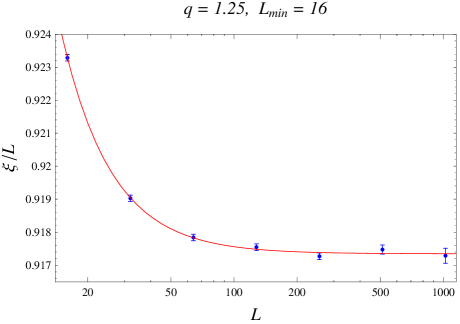 |
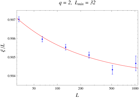 |
| (a) | (b) |
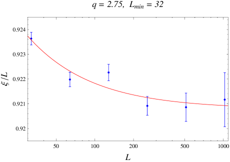 |
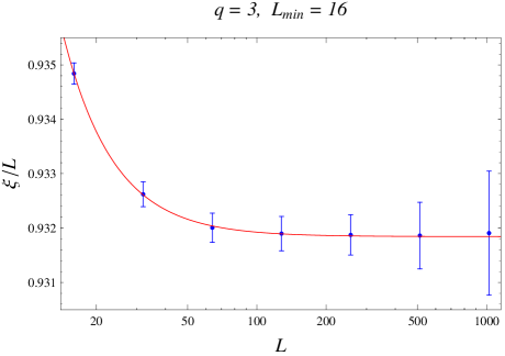 |
| (c) | (d) |
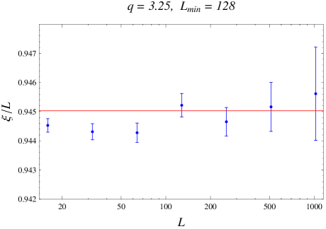 |
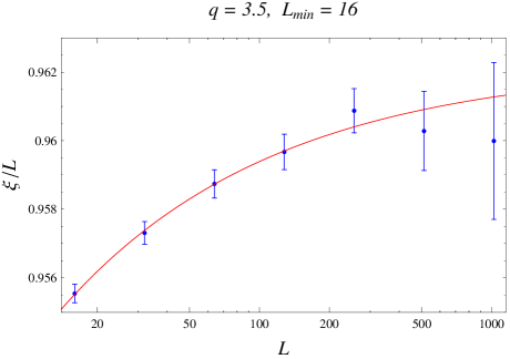 |
| (e) | (f) |
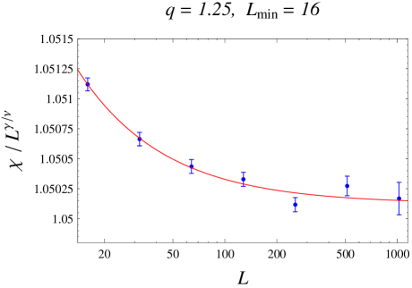 |
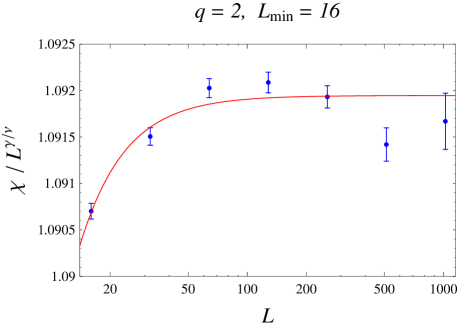 |
| (a) | (b) |
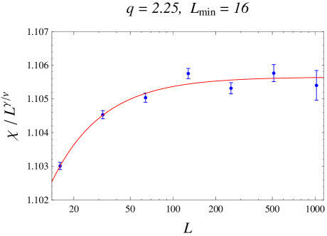 |
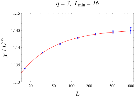 |
| (c) | (d) |
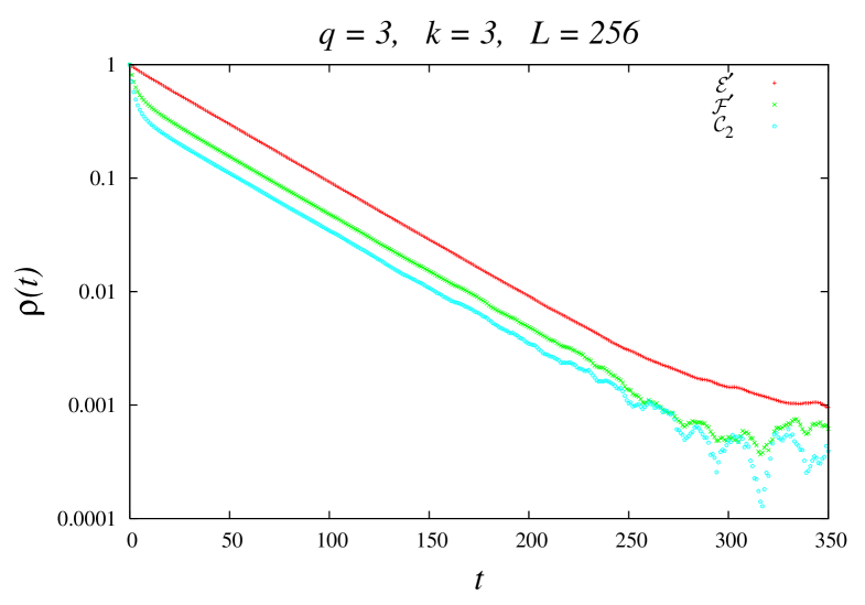
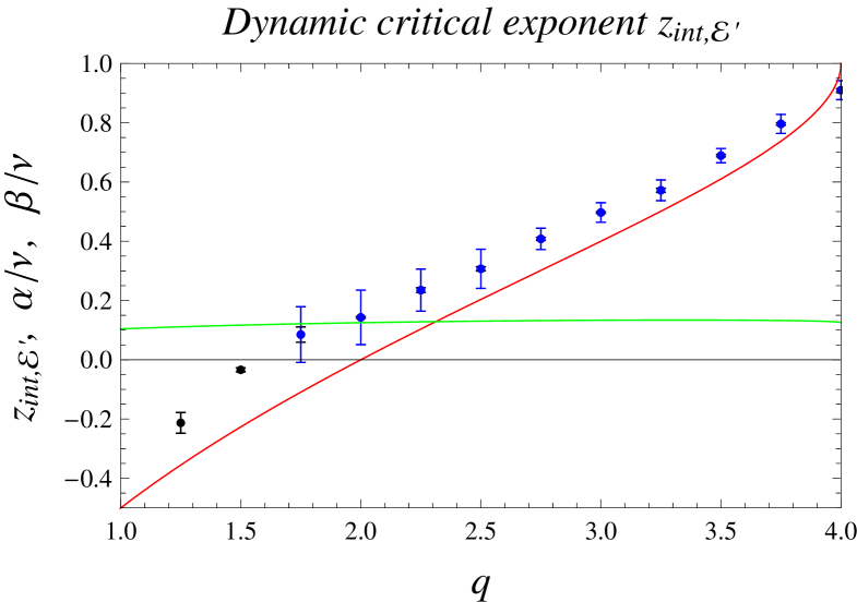
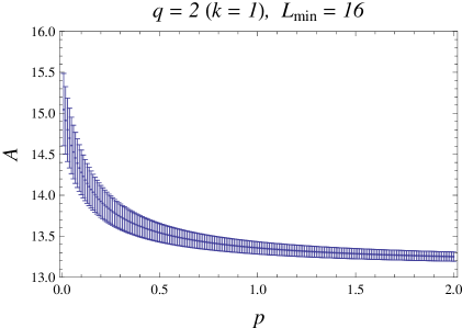 |
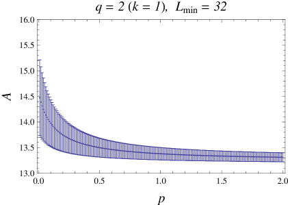 |
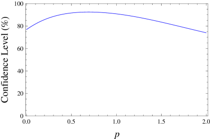 |
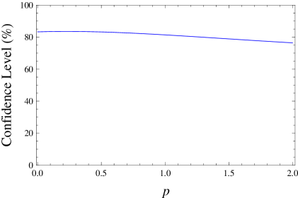 |
| (a) | (b) |
 |
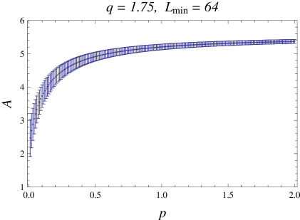 |
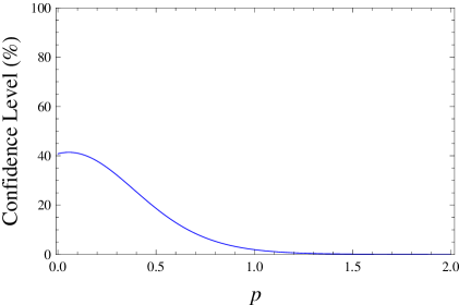 |
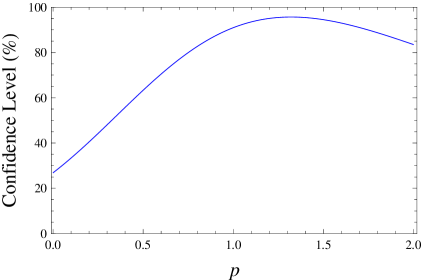 |
| (a) | (b) |
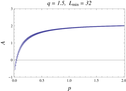 |
 |
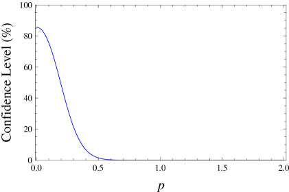 |
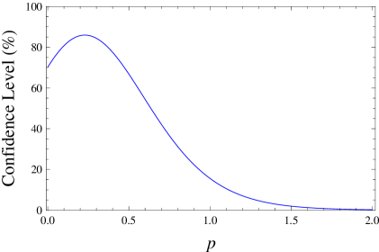 |
| (a) | (b) |
