Non-collinear Magnetic Order in the Double Perovskites:
Double Exchange on a Geometrically Frustrated Lattice
Abstract
Double perovskites of the form A2BB′O6 usually involve a transition metal ion, B, with a large magnetic moment, and a non magnetic ion B′. While many double perovskites are ferromagnetic, studies on the underlying model reveal the possibility of antiferromagnetic phases as well driven by electron delocalisation. In this paper we present a comprehensive study of the magnetic ground state and scales of the minimal double perovskite model in three dimensions using a combination of spin-fermion Monte Carlo and variational calculations. In contrast to two dimensions, where the effective magnetic lattice is bipartite, three dimensions involves a geometrically frustrated face centered cubic (FCC) lattice. This promotes non-collinear spiral states and ‘flux’ like phases in addition to collinear anti-ferromagnetic order. We map out the possible magnetic phases for varying electron density, ‘level separation’ , and the crucial B′B′ (next neighbour) hopping .
I Introduction
Double perovskites (DP) constitute a large family of materials dp-rev with molecular formula A2BB′O6, where A is an alkali or alkaline earth metal, and B and B′ are typically transition metals. Although double perovskites have been studied for decades Anderson1993197 , the discovery of high ferromagnetism and half-metallicity in Sr2FeMoO6 has led to renewed interest in their properties. Later, in a number of explorations it was discovered that these materials are candidates for various technological applications, e.g., in spintronics tokura (Sr2FeMoO6), magneto-dielectrics rogado:2005 ; umesh08 (La2NiMnO6), and magneto-optics molly (Sr2CrOsO6,Sr2CrReO6). Their properties are determined by the couplings on the B and B′ ions, the B and B′ valence state, and the structural order in the B-B′ lattice.
The magnetism in the DP’s arises from a combination of Hund’s coupling on the B, B′ ions and electron delocalisation. While there are important DP’s where both B and B′ are magnetic ions, in the current work we will restrict ourselves to materials where only one ion, B, say, is magnetic. For example, in Sr2FeMoO6 (SFMO) the B atom (Fe) is magnetic while B′ (Mo) is non magneticPhysRevLett.85.2549 . Even in this restricted class, a large variety of compounds can be realized by taking , or transition metals as B and B′, and alkaline earths or rare-earths as A. These lead to a variety of properties, e.g., high ferro(or ferri) magnetism (FM), with half-metallictopwaldd ; majewski05 or insulating krockenberger:020404 behaviour.
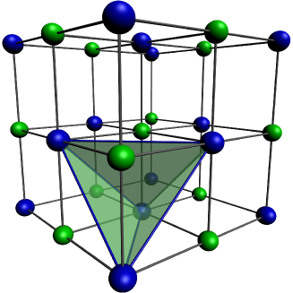
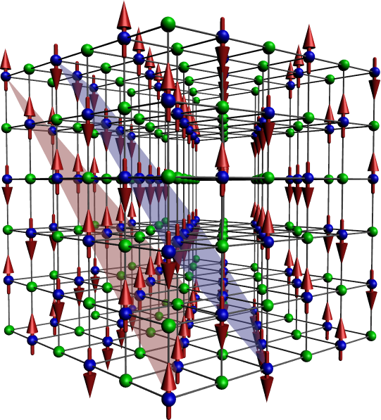
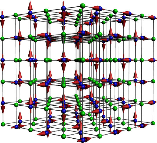
There have been several attempts at a theoretical understanding of the magnetism in these materials. These consist of (i) ab initio electronic structure calculations, and (ii) model Hamiltonian based approaches. The ab initio calculationsumesh08 ; molly ; PhysRevLett.85.2549 provide material specific information about the electronic structure and allow a rough estimatemandal:134431 of the . Unfortunately, these calculations are rather complicated for non-collinear magnetic phases that are likely in a frustrated magnetic lattice, see Fig.1. In such situations model Hamiltonian studies can provide some insight on possible ordered states.
Early model calculations for DP’s used dynamical mean field theory (DMFT) to estimate and the magnetic stability window PhysRevB.64.024424 ; PhysRevB.67.125119 , focusing on ferromagnetism. Earlier work on the classical Kondo lattice kp-pm-klm ; PhysRevB.51.3027 ; PhysRevB.62.13816 ; PhysRevB.64.054408 had revealed that variation in carrier density can lead to a wide variety of phases in a spin-fermion problem. Indeed, calculation sanyal:054411 in a two dimensional (2D) model of DP’s confirmed the existence of antiferromagnetic (AF), albeit collinear, phases. The ‘frustrated’ character of the three dimensional (3D) DP lattice raises the intriguing possibility of doping driven non collinear magnetic phases as well. Our study aims to explore this issue in detail.
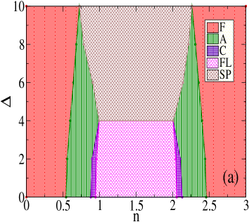
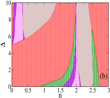
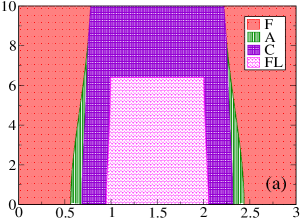
Our main results are the following. Using a combination of Monte Carlo and variational minimization, we map out the magnetic ground state (Fig.2) at large Hund’s coupling for varying electron density and B-B′ level separation. In addition to FM, and collinear A and C type order, the phase diagram includes large regions of non-collinear ‘flux’ and spiral phases and windows of phase separation. Modest B′B′ hopping leads to significant shift in the phase boundaries, and “particle-hole asymmetry”. We provide estimates of the of these non trivial magnetic phases.
II Model and method
Previous study of double perovskites in two dimensions sanyal:224412 revealed three collinear phases, namely FM, a diagonal stripe phase (FM lines coupled antiferromagnetically) and a ‘G type’ phase (up spin surrounded by down and vice versa). In 2D the B sub-lattice is square and bipartite, so there is no frustration. In a 3D simple cubic B lattice the counterparts of the 2D phases would be FM, A type (planar), C type (line like) and G type. The magnetic B ion lattice in the DP’s is, however, FCC which is non-bipartite, so while one can construct FM and planar A type phases, the C type phase is modified and the G type phase cannot exist.
Fig.1 briefly indicates why it is impossible to have an ‘up’() B ion to be surrounded by only ‘down’() B ions, i.e., the G type arrangement. Two B neighbours of a B ion are also neighbours of each other, frustrating G type order. The suppression of the G type phase, which occupies a wide window in 2D, requires us to move beyond collinear phases in constructing the 3D phase diagram. We will discuss the variational family in Section II.3.
II.1 Model
The alternating arrangement of B and B′ ions in the ordered cubic double perovskites is shown in Fig.1. We use the following one band model on that structure:
The correspond to the B ions and the to the B′. and are ‘onsite’ energy on the B and B′ sites respectively, e.g., the level energy of Fe and Mo in SFMO. is the chemical potential and is the total electron number operator. is the hopping amplitude between nearest neighbour B and B′ ions. We augment this model later to study first neighbour B′B′ hopping as well. is the (Hund’s) coupling between the B core spin and the conduction electron. We will use , and absorb the magnitude of in . are the Pauli matrices.
The model has parameters , , , and (or ). Since only the level difference matters, we set . We have set , and use so that the conduction electron spin at the B site is slaved to the core spin orientation. However, to keep the effective level difference between B and B′ sites finite we use the parameter , and explore the phases as a function of and . We will present results for and .
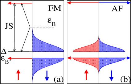
A schematic for the levels is shown in Fig.3. The structural unit cell of the system has 2 (one B, one B′) atoms, which amounts to 4 atomic levels (2 up spin, 2 down spin). The two spin levels at the B site are separated by and overlap with 2 spin degenerate levels of the B′ site at . We take the large limit, and take with in the range (0-10). One B band become centered at and second goes to . In this situation the down spin B and two B′ bands overlap while up spin B band is always empty. The relevant electron density window includes the lowest three bands, so our electron density will be in the range .
To get a general feel of the band structure of the particle hole symmetric case, we notice that we have three levels (excluding the highest level at which remains empty and is redundant for our purpose) in atomic limit. These include one spin slaved level at , and the two , , levels which overlap with the levels depending on the spin configurations. This overlap leads to electron delocalisation and band formation.
For the FM, Fig.3.(a), only one spin channel (say ) gets to delocalise through sites and forms two bands, separated by a band gap of , while other spin channel (say ) is localised at .
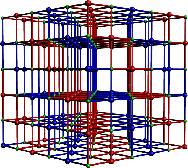
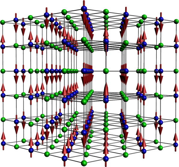
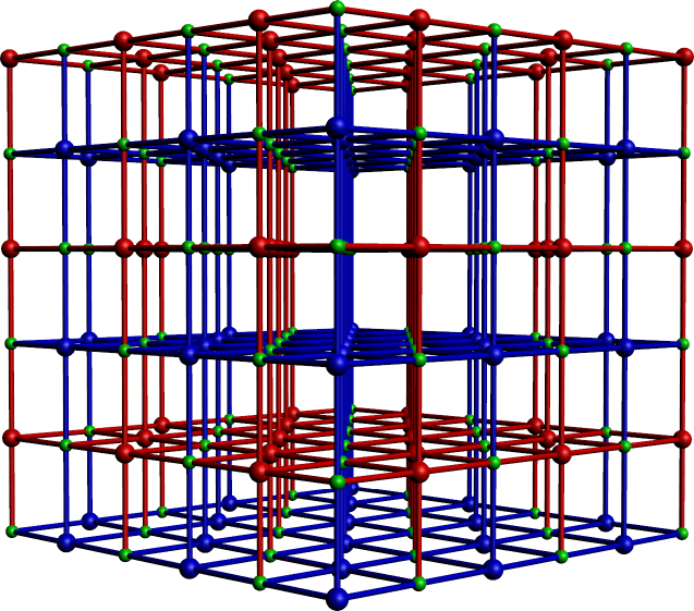
For collinear AF configurations, Fig.3.(b), the conduction path gets divided into two sub-lattices, such that each spin channel gets to delocalise in one sub-lattice (in which all the core spins point in same direction, making the sub-lattice ferromagnetic.) See Fig.4, and Fig.5 for the details of the conduction path. In one such sub-lattice, only one of the or delocalised, the other remains localised. The roles of and are reversed in going from one sub-lattice to other, as a result one gets spin-degenerate localised and dispersive bands for AF phases.
| Phase | Peak location in | |
|---|---|---|
| Ferromagnet ( FM) | (0,0,0),(,,) | |
| A-type antiferromagnet ( A) | (,, ),(,,) | |
| C-type antiferromagnet ( C) | (0,0,),(,,0) | |
| ‘flux’ ( FL) | ||
| phase | ||
| SP1 | ||
| SP2 | ||
| SP3 | ||
II.2 Monte Carlo method
The model involves spins and fermions, and if the spins are ‘large’, , they can be approximated as classical. This should be reasonable in materials like SFMO where . Even in the classical limit these spins are annealed variables and their ground state or thermal fluctuations have to be accessed via iterative diagonalisation of the electronic Hamiltonian. We use a ‘traveling cluster’ Monte Carlo (MC) method where the cost of a spin update is estimated via a small cluster Hamiltonian instead of diagonalising the whole system sanjeevTCA .
We typically use a system with the energy cost of a move estimated via a cluster built around the reference site. We principally track the magnetic structure factor
where denote thermal average.
Althogh the magnetic lattice is FCC, the electrons delocalise on the combined B-B′ system which is a cubic lattice. Hence we define our wave-numbers with respect to the full B-B′ lattice. As a result even a simple state like the ferromagnet corresponds to peaks at and and not just . This is because the spin field is also defined on B′ sites and it has to have zeros on these sites.
This complication, and the possibility of spiral phases, etc, mean that (i) there are multiple values which could be significant at low temperature, and (ii) the peaks could be small even in the ordered state. Combined with the intrinsic noise in MC data (which is enhanced due to a complex energy landscape, discussed later) it is sometimes difficult to identify complicated ordered phases. Therefore, to complement the MC results we have also used the following variational scheme.
II.3 Variational scheme
We explore a set of magnetic states, comparing their energy to locate the minimum within that family for a fixed set of electronic parameters. We use:
where and with if and if . , etc., are unit vectors in the corresponding directions.
The vector field is characterized by the two wave-vectors and . For a periodic configuration, these should be and , where ’s and ’s are integers, each of which take values in . There are ordered magnetic configurations possible, within this family, on a simple cubic lattice of linear dimension .
The use of symmetries, e.g., permuting components of , etc., reduces the number of candidates somewhat, but they still scale as . For a general combination of the eigenvalues of H cannot be analytically obtained because of the non trivial mixing of electronic momentum states. We have to resort to a real space diagonalisation. The Hamiltonian matrix size is () and the diagonalization cost is . So, a comparison of energies based on real space diagonalisation costs , possible only for .
We have adopted two strategies: (i) we have pushed this ‘’ scheme to large sizes via a selection scheme described below, and (ii) for a few collinear configurations, where Fourier transformation leads to a small matrix, we have compared energies on sizes .
First, scheme (i). For we compare the energies of all possible phases, to locate the optimal pair for each . We then consider a larger system with a set of states in the neighbourhood of . If we consider variation about each component of , etc, that involves states. The shortcoming of this method is that it explores only a restricted neighbourhood, dictated by the small size result. We have used within this scheme.
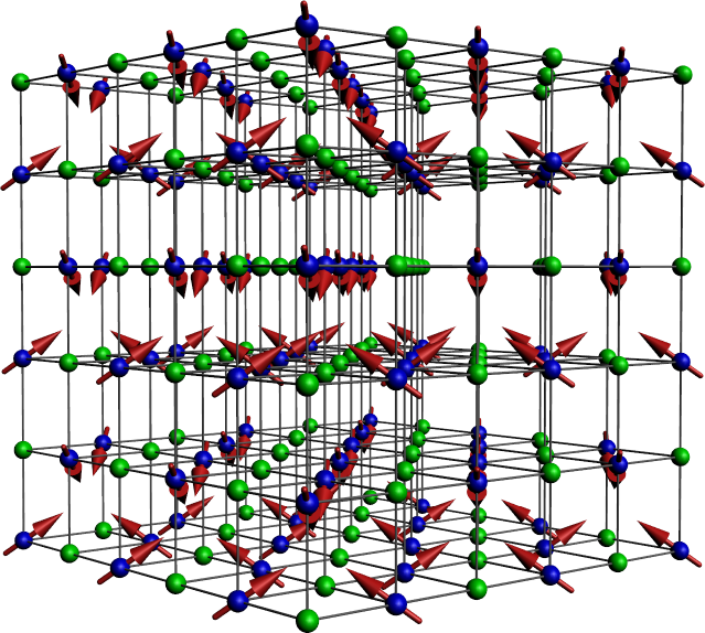
The phases that emerge as a result of the above process are (i) Ferromagnet (FM), (ii) A-type, (iii) C-type, (iv) ‘flux’, and (v) three spirals SP1,SP2,SP3. A-type is consists of () FM planes with alternate planes having opposite spin orientation (see Fig.4 top panel). If we convert each of these planes to alternating FM lines, so that the overall spin texture is alternating FM lines in all directions, we get C-type phase (see Fig.5.
The ‘flux’ phase is different from the spiral families described using period vectors . It is the augmented version of ‘flux’ phase used in cubic lattice double exchange model by Alonso et alPhysRevB.64.054408 (Table-I). It has spin-ice like structure, and is described by
The spiral SPn phases are characterised by comensurate values of (See Table 1 for details of periods and the S(q) peaks).
The simplest, SP1 can be viewed as -angle pitch in the , and directions. The other two spirals SP2 SP3 are respectively C-type and A-type modulations upon SP1. Just as flipping alternate planes in a FM leads to the A type phase, flipping the spins in the planes alternatively in SP1, leads to SP3. Analogously, flipping FM lines in a FM and leads to C-type order- and a similar exercise on SP1 leads to SP2. This modulation is also seen in the peaks of SP2 and SP3. See the Table 1, where all the three spirals have 4 S(q) peaks common, and SP2 and SP3 possess extra S(q) peaks of the A-type and C-type correlations.
In scheme (ii) we take collinear phases from the phase diagram via Monte-Carlo and variational scheme (i), and compare them on very large lattices. This does not require real space diagonalisation. The simple periodicity of these phases leads to coupling between only a few states. The resulting small matrix can be diagonalized for the eigenvalues and these summed numerically. We also did it for the ‘flux’ phase, where the resulting matrix is a bit larger, but still it gets us access to eigenvalues for the ‘flux’ phase on large lattices. The details of this calculation are discussed in Appendix A. Where the collinear phases (and ‘flux’) seem to dominate the phase diagram we compute phase boundaries by calculating the energy on very large lattices.
III Particle-hole symmetric case
The electrons move on the cubic lattice divided into two FCC sub-lattices each of which accommodate B and B′ sites. For each of these sub-lattice, one can define particle-hole transformation fazekas for B and B′ sub-lattices as and . This transforms the Hamiltonian as . When , this simplifies to which reflects in the phase diagram as the repetition of the phases after half-filling. Introducing the hopping destroys this symmetry, but a reduced symmetry still remains relating , which is reflected in the phase diagrams of particle-hole asymmetric case.
We first discuss the case of particle-hole symmetry, i.e, , and the case of in the next section. For each of these cases we first discuss the MC results since these are unbiased, though affected by finite size and the cluster update mechanism. This provides a feel for the relevant candidate states that we can explore more carefully within a variational scheme. It also provides an estimate of , not readily available within the variational scheme.
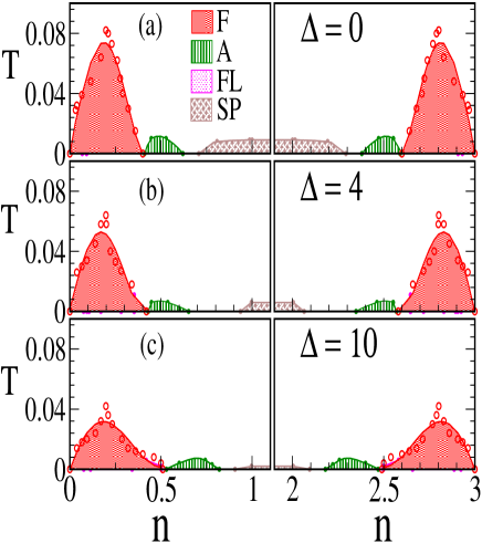
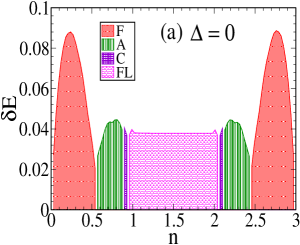
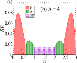
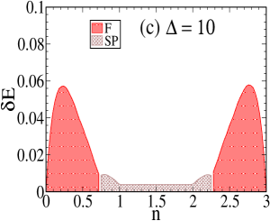
Following this we show the ground states and phase separation (PS) windows that emerge from the variational calculation for varying and . We also provide an alternate estimate of the “” of these phases by calculating the energy difference , that the system gains via magnetic ordering. Here is the electronic energy averaged over disordered (paramagnetic) spin configurations while is the energy of the magnetically ordered ground state, both at the same electron density . is the number of spins in the system. The phases that dominate the phase diagram are listed in Table-1, with the associated , and the peak locations in the structure factor.
III.1 Monte Carlo
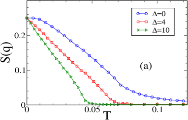
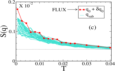
We studied a system using the cluster based update scheme. We used a large but finite to avoid explicitly projecting out any electronic states footnote1 , since that complicates the Hamiltonian matrix but allows only a small increase in system size. The magnetic phases were explored for and . An illustrative plot of peak features in as function of temperature , is shown in Fig.7 for some typical densities, where, for FM, S(qFM) shows monotonic decrease of Tc with increasing . For A-type and ‘flux’ phase, the S(q) data shows a number of sub-dominant q peaks whose number keeps increasing as we move to more complicated phases with increasing density.
Using the structure factor data, we establish the phase diagram for that is plotted in Fig.8. The Monte Carlo captures mainly three collinear phases, namely FM, A-type, and a phase. The phase corresponds to two FM up planes followed by two FM down planes and so forth. As the carrier density is increased via increasing , we find a FM phase followed by the A-type AF. A phase appears in a thin window surrounded by FM itself. We suspected that this as a finite size effect, and a comparison with the energy of the FM on larger lattices (), shows that the FM is indeed the ground state in the thermodynamic limit, and so we consider FM and collectively as FM only, and presence of is not indicated in the phase diagram.
The FM is stable at the ends of the density window, and its region of occurence is slowly enhanced as we increase , see Fig.2 as well. The however decreases with increasing since the degree of B-B′ mixing (and kinetic energy) decreases.
With further increase in the 2D system is known to make a transition to a line-like phase, and then a ‘G type’ phase (up spin surrounded by down, etc). In 3D one would expect the FM to change to a ‘planar’ (A type) phase, then a ‘line like’ (C type) phase and finally to a G type phase if possible. All of these are of course collinear phases, and geometric constraints may lead to non-collinear order as well.
While we do access the A type phase with some difficulty, our Monte Carlo cannot access the long range ordered C type phase. However, we see clear evidence of C type correlations in the structure factor. Comparing the energy of the ideal C type phase with the short range correlated phase that emerges from the MC we infer that such order is indeed preferred. However, we cannot estimate a reliable scale. In the next section we will see that the variational calculation confirms the stability of the C type, among collinear phases, in this density window, and will get a rough estimate of the from the energy .
The G type phase is geometrically disallowed on the B sub-lattice due to its FCC structure. An examination of the structure factor in the density window suggests ‘flux’ like correlations at small which evolves into a spiral at larger . The frustration reduces the of the phases in this density window compared to that of the FM. We studied the situation in 2D, where the system is unfrustrated, and the numbers below highlight the impact of frustration. In 2D, Monte Carlo results yield , while in 3D . We had focused on AF states at . If we compare the for 2D and 3D, the numbers come out to be and respectively footnote2 . The comparisons suggest a significant decrease in the binding energy (and hence ) of the AF phases relative to the FM as we move from 2D to 3D.
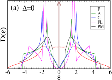
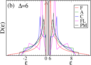
When , the electron delocalisation happens through B-B′-B paths only (see the conduction paths, for example of collinear phases A and C in Fig.4 and 5 respectively). In this cas all the phases have an atomic level located at in the limit . This is directly seen in the density of states (DOS) of these phase. In Fig.10 we show the DOS for the F, A, C, ‘flux’ and paramagnet phases. This dispersion-less level gives constant in density region . This feature, and several others, are modified by finite B′B′ hopping, which leads to broadening of this level. It makes the DOS of the various magnetic phases asymmetric (in energy) and also destroys the particle-hole symmetry in the phase diagram.
III.2 Variational scheme
Using the approach discussed earlier, we found the ground state configurations at different electron densities. In this set we also get certain spiral phases, which are small variations of FM, A, and C phases in the left and right part of the density window. Since in these parts Monte Carlo also gives (for FM, A) clean result, we interpret it as a finite size effect. To get convinced about it, we compare the energies of these collinear phases (FM, A, C) with all their neighboring modulations s, at various lattice sizes. We find that with increasing lattice size, the per particle energy difference between collinear phase, and lowest energy candidate with the neighboring ,, decreases, which convinces us that if we go to large enough lattice size, this difference will eventually vanish and the collinear phases (F,A,C) will be the relevant candidates.
We use a similar scheme for the middle part, however there no simple phase is suggested by this variational scheme (neither by Monte Carlo). The phases we propose for the middle density part based on this variational scheme are SP1, SP2, SP3, and ‘flux’. See the configurations in Fig.6 and details from Table 1.
In Fig.2, the magnetic ground state is shown for and (top and bottom). We see that for the phase diagram is symmetric in density. For small , in the range , we have FM, followed by A-type, C-type, and ‘flux’ phase. The order reverses as we go in the other half of the density window. The G-type phase which was largest stable phase in 2D (Fig.2 and Fig.5 in Ref. sanyal:054411 ) is almost taken over by the ‘flux’ phase. The stability of the ‘flux’ phase decreases with and it does not show up for .
In Fig.10, we show the DOS for F, A, C, ‘flux’ and PM phases. The upper and the lower panel correspond to and respectively. In all the phases, at all , there is a spike (delta function) at , which accounts for the non-dispersive level at .
For FM all the core spins are (say), so only spin electrons from B′ site get to delocalise while spin electrons remain localised at , which corresponds to the localised band in the sepctrum and the spike in the DOS. So the localised level in FM is an spin level. The nature of this localised level however changes when we go to AF phases. In collinear phases, its easy to understand the nature of this localised band. Take for example the case of A-type in Fig.4 down panel with conduction path. The lattice is divided into two sublattices (each of which are of layered zigzag shape), blue and red, such that, if (say) core spins in the sites in the blue sub-lattice are all , then the same in red sub-lattice are . As a result, in the blue sub-lattice, spin electrons get to delocalise, while spin electron remain localised. the opposite happens in the red sub-lattice. Since these lattices are disconnected from each other, one can separately diagonalise them. But each of this sub-lattice, however complicated in shape, is a FM, so it gives of the levels localised at , which will be spin in blue sub-lattice, while it will be spin in red sublattice. Since both the sub-lattices have same number of sites/unit cells, we get of the levels localised at but now spin degenerate. The delocalised states have also to be spin-degenerate, and their nature depends on the way the conduction paths divide the lattice into two sub-lattices.
For each spin channel the conduction paths are layered zigzag, 2 dimensional in the A type phase, while they are 3 dimensional in the C type phase.
This appearance of the localised band is not restricted to just the collinear phases, but also happens for non-collinear phases, and even the paramagent.
IV Particle-hole asymmetry
The model with only ‘nearest neighbour’ (BB′) hopping has a rich phase diagram. However, this has the artificial feature of a non dispersive level. In reality all materials have some degree of B′B′ hopping and we wish to illustrate the qualitative difference that results from this hopping. We explored two cases, and for these particle-hole asymmetric cases.
IV.1 Monte Carlo
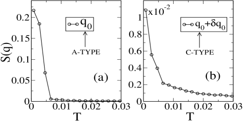
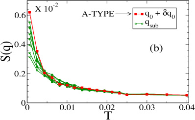
In Fig.11(a),(b) we show the structure factor data, at two densities, for (a) A type and (b) C type phases, to demonstrate one remarkable difference from the particle-hole symmetric case. As we saw earlier in Fig.7 for the structure factor data were very noisy for AF phases, with many sub-dominant q peaks around the central peak. The saturation value for the A-type peak in the symmetric case was , while now it is , close to the ideal value of . The sharp change in the structure factor makes the identification of the scale more reliable. Although inclusion of does not remove the noise completely, it is reduced over a reasonable part of the phase diagram.
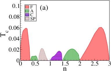
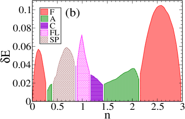
Fig.12(a) presents the phase diagram for and established from Monte Carlo, along with the from the variational approach (Fig.12(b)). In this case, the phases that appear as a function of density are FM, A type, spiral, C type, A type and FM again. For FM, the window of stability gets reduced in the left (low density) part but enhanced to almost full band ( to 3) in the right (high density) part. The phase appears again, but being a finite size artifact, is absorbed in the FM (and not shown). The is usually reduced, from the symmetric () case, as hopping provides conduction paths that are non-magnetic. There is a wider space with moderate for A type phase, located asymmetrically in density. Its more stable, in the right window, than left window, hence possessing relatively higher than left. The correlations of spiral and C type phases are also captured with relatively less noise, see Fig.11(b) for example of C-type correlation. Although S(q) data for these phases still contain some noise, so that we don’t get clean ground state here either. The phase diagram for and , can be obtained from transformation , i.e., reversing the density axis of Fig.12(a),(b).
IV.2 Variational scheme
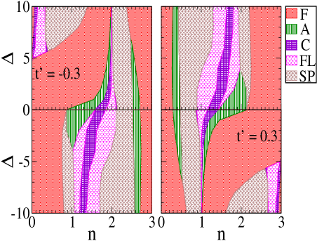
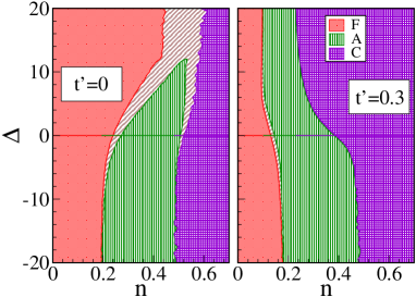
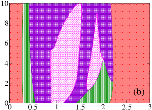
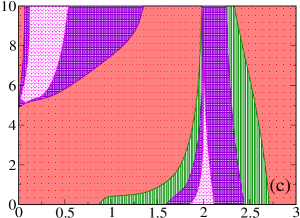
We employ the variational scheme discussed earlier and obtain the ground state phase diagram for is shown in Fig.13. Turning on has a significant effect on the phase diagram, when we use the case, Fig.2 top panel, for reference. The particle hole symmetry is destroyed at finite but a reduced symmetry still holds. The phase diagram is richer in the middle of the density window where crossing among various phases occurs at different densities. Due to the symmetry mentioned above it is enough to discuss the case with .
For the trends from MC are well reproduced by the variational scheme on large systems at . We observe reduced stability of FM at low density and enhancement at high density.
Note that the overall correspondence between the Monte Carlo and the variational approach is much better here than in the case, Fig. 8 and Fig. 9.
The A-type phase becomes very thin in the left, but unaffected by , while in right side it widens up in the low and gets replaced by the spiral quickly as we go up in . ‘flux’ and C-type both become stable for high with a gradual shift in the high density. For , at very small in the left and the middle part A-type and the spiral are major candidates with small window for C-AF and ‘flux’. The behaviour in this part is not very sensitive to sign of .
Focusing on , as go up from to the AF phases become less and less stable and are almost wiped out from the left part of the density, and FM becomes stable there. The largest stability window of FM occurs roughly near , where its stable upto . Going further with higher , FM looses its stability, from C type, ‘flux’ and spirals. However, there is very thin strip of stability of the FM in the band edge in the left part, and towards the middle density, there is re-entrance of the FM phase.
In the right part of the density, we have FM, A type and spiral. Increasing reduces the stability of A type to FM, making it vanish near , while FM window keeps increasing with .
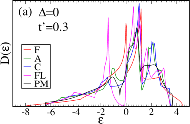
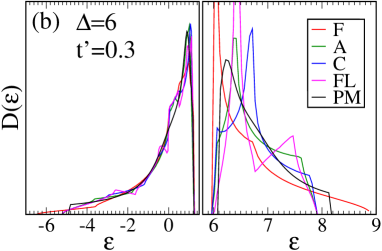
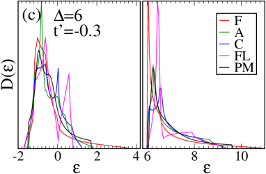
The DOS for the ordered F, A, C, ‘flux’ phase and the paramagnet are shown in Fig.14. (a) For , FM has the largest bandwidth, with paramagnet second largest. The band edges of A, C, ‘flux’ almost coincide both for small and large . (b) For the left band shows that all the phases seem to have ‘almost’ similar features in the DOS, while the right band shows distinct features of each of the phases, similar to DOS. (c) For however, has a disctint case. Here the lower edge of the band for FM, ‘flux’ and C coincide, and the DOS of ‘flux’, or C, is higher than FM, which explains why FM becomes unstable in the left side and taken by ‘flux’ and C, upon increasing .
We also estimate the phase separation boundaries between FM, A, C phases shown in Fig.15. For and for , we see that PS regions are significant, while they vanish for as we go down. For , (right panel) the PS boundaries are too narrow to be visible.
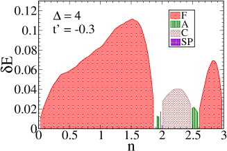
In Fig.16 we have shown the calculated for 203 size, for , with the large stability window of ferromagnet(See Fig.12). Here, though the and are non-zero, due to unusually large stability window, the (or ) is large.
To summarise, from the MC and variational data we learn that, apart from asymmetry in the phase diagram, collinear FM and A type phases become stable in wide density window. Their however is slightly reduced than the symmetric case. The S(q) data showing less noise for A, C type and spirals indicates that the energy landscape become ‘smoother’ by so that annealing process becomes easier to get to the ground state. The energy differences as well as MC estimated s show overall decrease with . This is understable as, by introducing we allow electrons to more on the ‘non-magnetic’ sub-lattice B′. Now the energy of any phase, depends on the energy gain via the hopping process. From the nearest hopping, this gain scales as subject to spin configurations, while the from the next nearest hopping, this gain simply scales as , and doens’t care upon spin configurations. So more we increase and , the more we are making the energy of the system insensitive to spin-configurations. The asymptotic limit of this is when every phase has same energy as paramagnet. That also explains why the phase seperation windows become very small with inclusion of .
In the couple of paragraphs below we try to create an understanding of how the phase diagram is affected by . There is’nt, unfortunately, an understanding of the effects over the entire density window, but we can at least motivate the changes at low density.
For , the FM loses its stability to AF phases even at low . That is puzzling since one would expect the FM phase to have the largest bandwidth. We recall that in the case, there is a localised band coming from B′ level for all the phases. The dispersion of this previously localised level causes the and to have a dependent separation, which was for all in the symmetric case. The separation for these levels in the asymmetric case is , which varies from , to in 3D. In 2D it varies from from , to .
If we consider the simpler 2D case for illustration, , which, for is minimum at k= while the maximum is at k=. For the opposite will happen. Thus, for k= and neighbouring states will experience enhanced mixing , while, the states near k= experience lower mixing. In the ferromagnet (both in 2D and 3D), the lowest eigenvalue corresponds to , while (for 2D) the G-type phase has lowest eigenvalues at . Therefore, for , the lowest eigenvalues of both the phases are enhanced but the band-edge of FM stays lower than G type. While in the other, the strongest mixing states are and , which aren’t at the edge for FM, its band-edge gets lower enhancement, while the band-edge of G type gets lowered. For a given , as we increase , a point comes where band edges of the FM and G, coincide. This is the point where FM loses its stability.
The same arguement can be extended to 3D, with C and flux phases, just the role of the s gets extended to 3D (e.g, etc), and the correction in the separation is instead of . In Fig. 17 we have shown the plot of lowest eigenvalues of F,A,C and flux phases with for
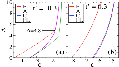
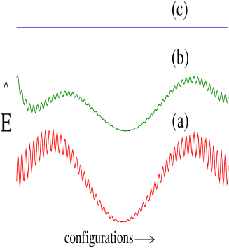
Finally, a comment (mainly a conjecture), Fig.18, on how the energy landscape of the DP model changes on addition of . We already know that the ‘binding energy’ and of magnetic phases reduce with increasing - but also that the ‘noise’ in the cooling process also reduces quickly.
If then the electrons could delocalise on the wide based band populating the non magnetic sites only. Magnetic order would make little difference to electronic energies and the ‘energy landscape’ in the space of spin configurations would be featureless, panel (c) in Fig.18. There are no global minima, i.e ordered states, and no local minima either. If then delocalisation takes place necessarily through the magnetic sites and the deep minima in configuration space represent ordered states while the ‘grassy’ features indicate shallow metastable states close to them. Our MC data probing AF states at suggests this picture, curve (a) in Fig.18. At intermediate the ordered states are shallower, but the metastable states seem to have been affected even more drastically, if our MC data, Fig.11, is to be taken seriously.
While the discussion above seems to be merely an analysis of trends in the MC annealing process, a simpler energy landscape would make the occurence of AF states more likely in the real materials as well.
V Discussion
The real double perovskites are multiband materials, involving additional interaction effects and antisite disorder beyond what we have considered in this paper. We feel it is necessary to understand in detail the phase diagram of the ‘simple’ model we have studied, and then move to more realistic situations. Below, we first provide a qualitative comparison of the trends we observe with experimental data, and then move to a discussion of additional interactions.
There are no clear experimental signatures of metallic AF phases yet, driven by the kind of mechanism that we have discussed. So, the comparison to experiments is, at the moment, confined to the scales dp-tc1 ; dp-tc2 etc, of the ferromagnetic DP’s. In a material like SFMO the electron density can be increased by doping La for Sr, i.e, compositions like Sr2-xLaxFeMoO6. This was tried dp-tc1 and the increased from 420K at to 490K at . SFMO has threefold degeneracy of the active, , orbitals while we have considered a one band model. When we create a correspondence by dividing the electron count by the maximum possible per unit cell (3 in our case, 9 in the real material), in our units corresponds to and to .
When , as a function of the peaks around , Fig.8, quite far from the experimental value. However, in the presence of and , Fig.16, the peak occurs above . So, modest can generate the ferromagnetic window that is observed, and produce a . For eV, this is in the right ballpark.
Unfortunately, attempts to increase via A site substitution also brings in greater antisite disorder (B-B′ interchange) and even the possibility of newer patterns of A site ordering (!) complicating the analysis. For example, one would try compositions of the form: A2-xABB′O6, where A and A′ have different valence in an attempt to change . The assumption is that the A′ only changes without affecting other electronic parameters, i.e, A′ ions do not order and remain in an alloy pattern. This may not be true. In fact, at , the material AA′BB′O6 may have a specific A-A′-B-B′ ordering pattern that affects electronic parameters in a non trivial way and one cannot understand this material as a perturbation on A2BB′O6. In such a situation one needs guidance from experiments and ab initio theory to fix electronic parameters as is varied. All this before one even considers the inevitable antisite (B-B′) disorder and its impact on magnetism vn-pm-af-asd.
VI Conclusions
We have studied a one band model of double perovskites in three dimensions in the limit of strong electron-spin coupling on the magnetic site. The magnetic lattice in the cubic double perovskites is FCC and increasing the electron density leads from the ferromagnet, through A and C type collinear antiferromagnets, to spiral or ‘flux’ phases close to half-filling. We estimate the of these phases, via Monte Carlo and variational calculation, and find the AF to be significantly suppressed compared to the 2D case. We attribute it to the geometric frustration on the FCC lattice. The introduction of B′B′ hopping significantly alters the phase diagram and scales and creates a closer correspondence to the experimental situation on DP ferromagnets.
Acknowledgements.
We acknowledge use of the high performance computing facility at HRI. PM was supported by a DAE-SRC Outstanding Research Investigator Award, and the DST India via the Indo-EU ATHENA project.Appendix A
Here we show how to calculate dispersion for selected ordered phases, which have relatively small unit cells. We define the unit cell for each phase, and go to space where the hamiltonian becomes block diagonal.
A.1 Spectrum for collinear phases
The Hamiltonian can be diagonalized by Fourier transformation We write the Hamiltonian as , where, is given by,
| (3) |
and is given by
| (4) |
The lattice vector is defined as with as the primitive lattice vectors (, , ), defining the periodicity of lattice with the 2 site unit cell. With this periodicity, the unit cell has one ”f” and one ”m” site at and respectively. Now doing a Fourier transform on ”” operators (similarly for ””s)
| (5) | |||
| (6) |
This simplifies the non-magnetic part as follows,
| (7) |
| (8) |
Which is reduced to block. the amplitudes and are just the cubic and FCC dispersions given by
Next, we have to simplify the part. For the collinear phases, can be expressed as
| (9) |
For FM, is trivially . For A-type, , while for C-type . Now, plugging this value of in and doing the Fourier transform for the , we get,
| (10) |
Now for FM, so becomes diagonal. Thus total hamiltonian still remains block, and the eigenvalues for the FM are solutions of the following block
| (11) |
For A-type and C-type phases, we get matrix elements connecting , so that now we get to solve following block
| (12) |
From these we obtain the spectrum for F,A,C phases on large () lattices, which can be used to calculate the density of states, phase diagram, phase separation windows etc.
A.2 Spectrum for the ‘flux’ phase
The unit cell for the ‘flux’ phase has 4, and 4 atoms lying on the corners of the cube.
![[Uncaptioned image]](/html/1105.0148/assets/x28.png)
The primitive lattice vectors become At finite , the same procedure (as for collinear phases) will reduce the hamiltonian into block. To make life a bit simple, we use the J limit on the hamiltonian for the ‘flux’ phase, which is same as used in sanyal:054411 except its the 3D version.
This gives us 4 spinless levels and 8 levels in the unit cell, which upon simplification reduces to block. With the basis The hamiltonian breaks into block given as follows
References
- [1] For reviews, see D. D. Sarma, Current Op. Solid St. Mat. Sci.,5, 261 (2001), D. Serrate, J. M. de Teresa and M. R. Ibarra, J. Phys. Cond. Matt. 19, 023201 (2007).
- [2] Mark T. Anderson, Kevin B. Greenwood, Gregg A. Taylor, and Kenneth R. Poeppelmeier. Progress in Solid State Chemistry, 22, 197 (1993).
- [3] K.-I. Kobayashi, T. Kimura, H. Sawada, K. Terakura, and Y. Tokura. Nature (London) 395, 677, (1998).
- [4] M.A. Subramanian N.S. Rogado, J. Li. Advances in Materials 17, 2225 (2005).
- [5] Hena Das, Umesh V. Waghmare, T. Saha-Dasgupta, and D. D. Sarma. Phys. Rev. Lett. 100, 186402, (2008).
- [6] Hena Das, Molly De Raychaudhury, and T. Saha-Dasgupta. Appl. Phys. Lett. 92, 201912 (2008).
- [7] D. D. Sarma, Priya Mahadevan, T. Saha-Dasgupta, Sugata Ray, and Ashwani Kumar. Phys. Rev. Lett. 85, 2549 (2000).
- [8] J. B. Philipp, P. Majewski, L. Alff, A. Erb, R. Gross, T. Graf, M. S. Brandt, J. Simon, T. Walther, W. Mader, D. Topwal, and D. D. Sarma. Phys. Rev. B 68, 144431 (2003).
- [9] P. Majewski, S. Geprägs, A. Boger, M. Opel, A. Erb, R. Gross, G. Vaitheeswaran, V. Kanchana, A. Delin, F. Wilhelm, A. Rogalev, and L. Alff. Phys. Rev. B 72, 132402 (2005).
- [10] Y. Krockenberger, K. Mogare, M. Reehuis, M. Tovar, M. Jansen, G. Vaitheeswaran, V. Kanchana, F. Bultmark, A. Delin, F. Wilhelm, A. Rogalev, A. Winkler, and L. Alff. Phys. Rev. B 75, 020404 (2007).
- [11] Tapas Kumar Mandal, Claudia Felser, Martha Greenblatt, and Jürgen Kübler. Phys. Rev. B 78, 134431 (2008).
- [12] A. Chattopadhyay and A. J. Millis. Phys. Rev. B 64, 024424 (2001).
- [13] K. Phillips, A. Chattopadhyay, and A. J. Millis. Phys. Rev. B 67, 125119 (2003).
- [14] M. Hamada and H. Shimahara. Phys. Rev. B 51, 3027 (1995).
- [15] D. F. Agterberg and S. Yunoki. Phys. Rev. B 62, 13816 (2000).
- [16] J. L. Alonso, J. A. Capitán, L. A. Fernández, F. Guinea, and V. Martín-Mayor. Phys. Rev. B 64, 054408 (2001).
- [17] K. Pradhan and P. Majumdar, Europhys. Lett. 85, 37007 (2009).
- [18] Prabuddha Sanyal and Pinaki Majumdar. Phys. Rev. B 80, 054411 (2009).
- [19] Sanjeev Kumar and Pinaki Majumdar. EPJ B50, 571 (2006).
- [20] Prabuddha Sanyal, Hena Das, and T. Saha-Dasgupta. Phys. Rev. B 80, 224412 (2009).
- [21] Shuai Dong, Rong Yu, Seiji Yunoki, J.-M. Liu, and Elbio Dagotto. Phys. Rev. B 78, 155121 (2008).
- [22] We have worked on , so J has to be large compaired to it. We used J = 1000, as the atomic bands which, for finite J, are actually dispersive (of band-width ) become actually atomic to required numerical accuracy.
- [23] We campared ratio of the maximum of and maximum of in the density window, for and
- [24] Patrik Fazekas, Lecture Notes on Electron Correlation and Magnetism, Chapter 4.5, World Scientific.
- [25] J. Navarro, C. Frontera, L. Balcells, B. Martinez, and J. Fontcuberta, Phys. Rev. B64, 092411 (2001).
- [26] B.-G. Park, Y.-H. Jeong, and J.-H. Park, J. H. Song, J.-Y. Kim, H.-J. Noh, H.-J. Lin and C. T. Chen, Phys. Rev. B79, 035105 (2009).
- [27] Viveka Nand Singh and Pinaki Majumdar, arXiv:1009.1709.