Finding All the Stationary Points of a Potential Energy Landscape via Numerical Polynomial Homotopy Continuation Method

Abstract

The stationary points (SPs) of a potential energy landscape play a crucial role in understanding many of the physical or chemical properties of a given system. Unless they are found analytically, there is, however, no efficient method to obtain all the SPs of a given potential. We introduce a novel method, called the numerical polynomial homotopy continuation (NPHC) method, which numerically finds all the SPs, and is embarrassingly parallelizable. The method requires the non-linearity of the potential to be polynomial-like, which is the case for almost all of the potentials arising in physical and chemical systems. We also certify the numerically obtained SPs so that they are independent of the numerical tolerance used during the computation. It is then straightforward to separate out the local and global minima. As a first application, we take the XY model with power-law interaction which is shown to have a polynomial-like non-linearity and apply the method.

Introduction: A Potential energy landscape (PEL) is the hyper-surface of some given potential $V(\vec{x})$, with $\vec{x}=(x_{1},x_{2},...,x_{N})$ being the variables (e.g., position coordinates, fields etc.). Studying the stationary points (SPs), defined by the solutions of the system of $N$ equations $\frac{\partial V(\overrightarrow{x})}{\partial x_{i}}=0,i=1,...,N$, of the PEL is crucial in learning many physical or chemical properties of the system described by $V(\vec{x})$. The SPs are classified according to the number of negative eigenvalues of the Hessian matrix $\mathcal{H}$ evaluated at each SP: the SPs with no negative eigenvalue are called minima and the SPs with at least one negative eigenvalue are called saddles. In statistical mechanics, for example, the stationary points of the PEL have been shown to be directly related to the non-analyticity of thermodynamic quantities (i.e., phase transitions) in the respective models Kastner (2008); the global minimum of a spin glass model is invaluable for studying its equilibrium properties. In theoretical chemistry, studying the properties of the PEL of supercooled liquids and glasses has been a very active area of research Wales (2004); Collins et al. (2011), specifically, in the study of Kramer’s reaction rate theory for the thermally activated escape from metastable states, and the computation of various physical quantities like the diffusion constant using the minima of the PEL, etc. Wales (2004). In string theory, the SPs of the PEL of various supersymmetric potentials correspond to the so-called string vacua. A lot of current activities in the string phenomenology areas have been focused on developing different methods to find these string vacua Gray et al. (2009, 2006, 2007).

If all SPs are found analytically for the given $V(\overrightarrow{x})$, then the problem is settled, obviously. But if the analytical solutions are intractable, then one has to rely on alternative methods. Though finding SPs is of the utmost importance in so many areas, there do not exist many rigorous methods to find SPs, compared to the number of methods for minimizing a potential.

One such method is the gradient-square minimization method in which one minimizes $W=|\nabla V(\overrightarrow{x})|^{2}$ using some traditional numerical minimization method such as Conjugate Gradient, Simulated Annealing, etc. Angelani et al. (2000); Broderix et al. (2000). The minima of $W$, with further restriction that $W=0$, are the SPs of $V(\overrightarrow{x})$. However, there also exist minima of $W$ where $W>0$, and it has been shown that the number of these non-SPs grow as the system size increases Doye and Wales (2002); Wales and Doye (2003), thus making the method inefficient.

The Newton-Raphson method (and its sophisticated variants) may also be used to solve the system of $N$ non-linear equations $\frac{\partial V(\overrightarrow{x})}{\partial x_{i}}=0,i=1,...,N$. Here, an initial random guess is fed and then refined to a given numerical precision to obtain a solution of the system Grigera et al. (2002); Doye and Wales (2002). However, this method still suffers the major drawbacks of the gradient-square minimization method, namely, the possible existence of large basins of attraction may lead us to repeatedly obtain the same SPs and, more importantly, no matter how many times we iterate the respective algorithms with different initial guesses, we are never sure if we have found all SPs.

If the system of stationary equations has polynomial-like non-linearity, then the situation is a bit better: in the string theory community, for such a system of equations, the symbolic methods based on the Gröbner basis technique are used to solve the system Gray et al. (2006, 2009, 2007) which ensure that all the SPs are obtained when the computation finishes. Roughly speaking, for a given system of multivariate polynomial equations (which is known to have only isolated solutions), the so-called Buchberger Algorithm (BA) or its refined variants can compute a new system of equations, called a Gröbner basis, in which the first equation only consists of one of the variables and the subsequent equations consist of increasing number of variables. The solutions of the new system remain the same as the original system, but the former is easier to solve. This method apparently resolves all of the above mentioned problems, however, there are a few other problems: the BA is known to have suffered from the exponential space complexity, i.e., the memory (Random Access Memory) required by the machine blows up exponentially with the number of variables, equations, terms in each polynomial, etc.). So even for small sized systems, one may not be able to compute a Gröbner basis. It is also inefficient for the systems with irrational coefficients. Furthermore, the BA is highly sequential.

In this Letter, we present the numerical polynomial homotopy continuation (NPHC) method which solves all the above problems for systems of equations with polynomial-like non-linearity. Numerical continuation methods have been around for some time Allgower and Georg (1979) and the polynomial homotopy continuation method has also been an active area of research Sommese and Wampler (2005); Li (2003) (see Mehta (2009); Mehta et al. (2009) for the earlier account on the NPHC method for various areas in theoretical physics). As with the Gröbner basis technique, the method extensively uses concepts from complex algebraic geometry and hence we allow the variables to take values from the complex space, even if the physically important solutions are only the real ones. So long as a system of polynomial equations is known to have only isolated solutions, the NPHC guarantees that we obtain all complex solutions of the system, from which all the real solutions can subsequently be filtered out.

Numerical Polynomial Homotopy Continuation Method: Here we introduce the NPHC method to solve a system of multivariate polynomial equations. Specifically, we consider a system $P(\vec{x})=0$ which is known to have isolated solutions and where $P(\vec{x})=(\frac{\partial V(\vec{x})}{\partial x_{1}},\dots,\frac{\partial V(\vec{x})}{\partial x_{N}})$. Now, the Classical Bézout Theorem asserts that for a system of $N$ polynomial equations in $N$ variables that is known to have only isolated solutions, the maximum number of solutions in $\mathbb{C}^{N}$ is $\prod_{i=1}^{N}d_{i}$, where $d_{i}$ is the degree of the $i$th polynomial. This bound is called the classical Bézout bound (CBB).

Based on the CBB, a homotopy can be constructed as $H(\vec{x},t)=\gamma(1-t)Q(\vec{x})+t\,P(\vec{x})=0$, where $\gamma$ is a random complex number. The new system $Q(\vec{x})=(q_{1}(\vec{x}),\dots,q_{N}(\vec{x}))$, called the start system, is a system of polynomial equations with the following properties: (1) the solutions of $Q(\vec{x})=H(\vec{x},0)=0$ are known or can be easily obtained. The solutions of $Q(\vec{x})=0$ are called start solutions; (2) the number of solutions of $Q(\vec{x})=H(\vec{x},0)=0$ is equal to the CBB of $P(\vec{x})=0$, (3) the solution set of $H(\vec{x},t)=0$ for $0\leq t\leq 1$ consists of a finite number of smooth paths, each parametrized by $t\in[0,1)$, and (4) every isolated solution of $H(\vec{x},1)=P(\vec{x})=0$ can be reached by some path originating at a solution of $H(\vec{x},0)=Q(\vec{x})=0$. We can then track all the paths corresponding to each start solution from $t=0$ to $t=1$ and reach (or diverge from) $P(\vec{x})=0=H(\vec{x},1)$. It is rigorously shown that for a generic value of complex $\gamma$, all paths are regular for $t\in[0,1)$, i.e., there is no singularity along the path Sommese and Wampler (2005). By implementing an efficient path tracker algorithm, such as the Euler’s predictor and Newton’s corrector method, all isolated solutions of $P(\vec{x})=0$ can be obtained. We do not delve into the discussion of the actual path tracker algorithms used in practice in this Letter, except mentioning that in the path tracker algorithms used in practice, almost all apparent difficulties have been resolved, such as tracking singular solutions, multiple roots, solutions at infinity, etc.Sommese and Wampler (2005).

As a trivial illustration, let us take the univariate polynomial, $P(x)=x^{2}-5=0$, from Sommese and Wampler (2005). To find its solutions, we may for example choose $Q(x)=(x^{2}-1)$ as our start system as it satisfies the twin criteria that it has the same number of solutions as the CBB of $P(x)$ and is also easily solved to obtain the start solutions $x=\pm 1$. (Note that, more generally, $Q(\vec{x})=(x_{1}^{d_{1}}-1,\dots,x_{N}^{d_{N}}-1)$ is the simplest choice as a start system for the multivariate case.) The problem of getting all solutions of $P(x)=0$ now reduces to simply tracking the solutions of $H(x,t)=0$ from $t=0$ to $t=1$ so that the paths beginning at $x=\pm 1$ lead us to the actual solutions $x=\pm\sqrt{5}$. Note that, in general, if there are more start solutions than actual solutions, then the remaining paths diverge as $t$ approaches $1$.

There are several sophisticated computational packages such as PHCpack Verschelde (1999), Bertini Bates et al. and HOM4PS2 Lee et al. (2008) which can be used to solve systems of univariate and, more importantly, multivariate polynomial equations, and are available as freeware. For the sake of completeness, the solutions of the above mentioned univariate equation are $x=\pm(2.236067977+i\,10^{-10})$, i.e., $\pm\sqrt{5}$ up to the numerical precision.

Since each path can be tracked independently of all others, the NPHC is known as being embarrassingly parallelizable, a feature that makes it very efficient.

For the multivariate case, a solution is a set of numerical values of the variables which satisfies each of the equations with a given tolerance, $\triangle_{\mbox{sol}}$ ($\sim 10^{-10}$ in our set up). Since the variables are allowed to take complex values, all the solutions come with real and imaginary parts. A solution is a real solution if the imaginary part of each of the variables is less than or equal to a given tolerance, $\triangle_{\mathbb{R}}$ ($\sim 10^{-7}$ is a robust tolerance for the equations we will be dealing with in the next section, below which the number of real solutions does not change). All these solutions can be further refined with an arbitrary precision up to the machine precision.

The obvious question at this stage would be if the number of real solutions depend on $\triangle_{\mathbb{R}}$. To resolve this issue, we use a very recently developed algorithm called alphaCertified which is based on the so-called α-theory to certify the real non-singular solutions of polynomial systems using both exact rational arithmetic and arbitrary precision floating point arithmetic Hauenstein and Sottile (2010). This is a remarkable step, because using alphaCertified we can prove that a solution classified as a real solution is actually a real solution independent of $\triangle_{\mathbb{R}}$, and hence these solutions are as good as the exact solutions.

A First Application: As a first application, we choose the XY model with long range power-law (algebraically decaying) interaction, defined as $V(\vec{\theta})=K\sum_{i=1}^{N}\sum_{j=1}^{\frac{(N-1)}{2}}\frac{1-\cos(\theta_{i}-\theta_{i+j})}{j^{\alpha}},$ where $N$ is odd for our purposes, the normalization constant $K=(2\sum_{j=1}^{\frac{(N-1)}{2}}\frac{1}{j^{\alpha}})^{-1}$, and $\alpha\in[0,\infty)$ Kastner (2010). $\alpha=0$ reproduces the mean-field XY model and $\alpha\rightarrow\infty$ reproduces the nearest-neighbour coupling XY model for which all the SPs are analytically obtained recently Mehta (2009); von Smekal et al. (2007); Mehta and Kastner (2011). We choose $\alpha=0.75$ for which the coefficients take values from $\mathbb{R}$, unlike for example $\alpha=1$ for which the integers are rational numbers. Hence, we are already in the domain of problems where the Gröbner basis technique is inefficient. We impose periodic boundary condition, i.e., $\theta_{k+N}=\theta_{k}$. Spin glass models with power-law interaction have gained a huge interest recently Katzgraber et al. (2010). The chosen model is one of the simplest models of this kind with a continuous symmetry. The model is also known as the Kuramoto model with power-law interaction. The stationary equations are $\frac{\partial V(\vec{\theta})}{\partial\theta_{k}}=K\sum_{j=1}^{\frac{(N-1)}{2}}(\frac{\sin(\theta_{k}-\theta_{k+j})+\sin(\theta_{k}-\theta_{k-j})}{j^{\alpha}})=0,$ for $k=1,\dots,N$. To get rid of the global rotation symmetry $\theta_{k}\rightarrow\theta_{k}+\phi$ where $\phi\in\mathbb{R}$, we fix one of the angles, say $\theta_{N}=0$, and remove the $N$th equation out of the system, as done in Mehta and Kastner (2011); Mehta (2009). Kastner in Kastner (2010) used a specific class of known solutions, called the stationary wave solutions, i.e., $\theta_{m}^{(n)}=\frac{2\pi mn}{N}$, where $m,n\in\{1,\dots,N$}. Below we find that there are many more solutions for this model.

The above system of equations is not apparently a system of polynomial equations. But we can transform it into one Mehta (2009); Mehta et al. (2009) by first using the trigonometric identities, $\sin(\theta_{k}-\theta_{k+j})=\sin\theta_{k}\cos\theta_{k+j}-\sin\theta_{k+j}\cos\theta_{k}$ etc.; abbreviating each $\sin\theta_{k}=s_{k}$ and $\cos\theta_{k}=c_{k}$, in all the $N-1$ equations; and finally adding $N-1$ additional constraint equations as $s_{k}^{2}+c_{k}^{2}-1=0$, for $k=1,\dots,N-1$, we get a system of $2(N-1)$ polynomial equations consisting of $2(N-1)$ algebraic variables $c_{k}$s and $s_{k}$s as below:

$$K\sum_{j=1}^{\frac{(N-1)}{2}}\frac{(s_{k}c_{k+j}-s_{k+j}c_{k}+s_{k}c_{k-j}-s_{k-j}c_{k})}{j^{\alpha}}=0,$$

$$s_{k}^{2}+c_{k}^{2}-1=0,$$ (1)

for $k=1,\dots,N-1$. The removal of the global rotation symmetry ensures that the system will have only isolated solutions. We can now use the NPHC to solve the Eqs. (1) for all the $s_{k}s$ and $c_{k}$s; filter the real solutions out using the above mentioned tolerances; and finally get the original $\theta$-variables back by $\theta_{k}=\tan^{-1}(\frac{s_{k}}{c_{k}})\in(-\pi,\pi]$, for all $k=1,\dots,N-1$. The results are as follows.

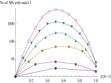
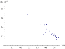
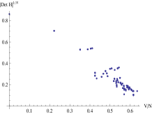
Firstly, the number of SPs for $N=3,5,7,9,11,13$ are $6,20,168,972,4774,24830$, respectively. The left panel in Figure 1 shows the number of SPs as a function of $N$. The SPs for different models with similar sizes have been studied using the gradient minimization and Newton-Raphson’s methods, though the final number of SPs is always open to debate Doye and Wales (2002); Wales and Doye (2003), whereas using the NPHC method we can find all the SPs with confidence. In the gradient minimization method, it is difficult to obtain the SPs with higher indices Doye and Wales (2002). In the NPHC, however, all the SPs are treated equally irrespective of their indices. The right panel in Figure 1 shows the index $I/(N-1)$ vs number of SPs for a given $N$. Apparently, the number of minima grows linearly in this model, which is contrary to the conventional wisdom Wales and Doye (2003); Doye and Wales (2002). However, the number of SPs indeed grows exponentially with increasing system size as expected Wales and Doye (2003); Doye and Wales (2002). We also observe that the global minimum is always the configuration with all $\theta_{i}=0,i=1,\dots,N-1$, and that at the global minimum, the energy density $V/N$ is zero. In Figure 2, we plot $V/N$ vs $I$ for $N=7,9,11,13$. The apparent non-linear relation between these two quantities in the plots show a different behaviour to the linear relationship observed for the Lennard-Jones models.

Figure 1: The left panel is the plot for $N$ vs no. of SPs: the circles, squares and diamonds represent data points for the algebraic decaying XY model, the one-dimensional nearest-neighbour XY model for periodic Mehta and Kastner (2011); Mehta (2009) and anti-periodic conditions von Smekal et al. (2007), respectively. The lines are drawn for a guide to the eyes. The right panel is the plot for index $I$ vs no of SPs with index $I$. From top to bottom, $N=13,11,9,7,5,3$. The normalization on $I$ is $N-1$ since we have taken $\theta_{N}=0$.

Figure 2: Plot for $V/N$ vs index density, starting from top left corner $N=7,9,11,13$, respectively.

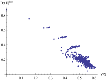
Although it is quite difficult to claim any result in the thermodynamic limit using such small size systems, we note that the minimum value of the $|\mbox{Det}\mathcal{H}|^{1/N}$ is always either at the SPs for which all $\theta_{i}\in\{0,\pi\}$ for all $i=1,\dots,N-1$, or for the SPs for which $\theta_{i+1}-\theta_{i}=\frac{2\pi k}{N}\mbox{ mod }2\pi$ for all $i=1,\dots,N$, with $k$ being an integer. Using a recently spelled out condition for a class of spin-glass models to have phase transition, that $|\mbox{Det }\mathcal{H}|^{1/N}$ evaluated at a class of stationary points tend to go to zero at the critical energy in the $N\rightarrow\infty$ limit, the phase transition in our model would occur at this specific class of solutions Nardini and Casetti (2009). For $N=7,9,11,13$, the corresponding plots are drawn in Figure 3 where the plot has started being filled up by densely populated points around the critical energy density $V/N\sim 0.5$. Hence, we have reproduced the results that Kastner worked out from other approach in Kastner (2010) by just studying these small size systems. These particular SPs are usually neither minima nor maxima.

Figure 3: Plot of $V/N$ vs $|\mbox{Det }\mathcal{H}|^{1/N}$ starting from upper left corner for $N=7,9,11,13$, respectively. Though these small sized systems can in no way be considered as representatives of the model in the thermodynamic limit, we still see the expected singularity of $|\mbox{Det }\mathcal{H}|^{1/N}$ at $V/N\rightarrow 0.5$.

It would be interesting to get all the SPs for $\alpha\in(1,2]$, find out the relevant SPs for the phase transition and extrapolate the analysis in the thermodynamic limit as suggested in Kastner (2010). Verifying a recent conjecture that the critical energy density of a class of spin glass models can be computed using the Ising-like SPs only (seeCasetti et al. (2011) for the definition of these SPs and the conjecture), will also be another important application of the NPHC method.

In this Letter, we have described and applied a novel method, called the numerical homotopy continuation (NPHC) method, that finds all SPs of a given potential, provided that the potential has polynomial-like non-linearity. As shown in this Letter, even if the given potential is not apparently in the polynomial form, its stationary equations could be transformed into a polynomial form by adding suitable constraint equations. So the method is very widely applicable. The ability of finding all SPs and it being completely parallelizable makes the method quite promising to study many areas of theoretical physics and chemistry, for example, finding all the SPs and hence all the minima of the Lennard-Jones potential and its numerous variants; to obtain the string vacua of the models for which the symbolic algebraic geometry methods fail due to their algorithmic complexities; to study phase transitions in various spin glass models with the above mentioned criterion on the hessian determinant etc. We anticipate that this work will give a thrust to the current research in the related areas.