The RAdial Velocity Experiment (RAVE): Third Data Release

Abstract

We present the third data release of the RAdial Velocity Experiment (RAVE) which is the first milestone of the RAVE project, releasing the full pilot survey. The catalog contains $83\,072$ radial velocity measurements for $77\,461$ stars in the southern celestial hemisphere, as well as stellar parameters for $39\,833$ stars. This paper describes the content of the new release, the new processing pipeline, as well as an updated calibration for the metallicity based upon the observation of additional standard stars. Spectra will be made available in a future release. The data release can be accessed via the RAVE webpage: http://www.rave-survey.org.

1 Introduction

A detailed understanding of the Milky Way, from its formation and subsequent evolution, to its present-day structural characteristics, remains key to understanding the cosmic processes that shape galaxies. To achieve such a goal, one needs access to multi-dimensional phase space information, rather than restricted (projected) properties - for example, the three components of the positions and the three components of the velocity vectors for a given sample of stars. Until a decade ago, only the position on the sky and the proper motion vector was known for most of the local stars. Thanks to ESA’s Hipparcos satellite (Perryman et al., 1997), the distance to more than $100\,000$ stars within a few hundred parsecs has been measured, allowing one to recover precise positions in the local volume (a sphere roughly 100 pc in radius centered on the Sun). However, the $6^{\rm th}$ dimension of the phase space was still missing until recently, when Nordström et al. (2004) and Famaey et al. (2005) released radial velocities for subsamples of respectively $14\,000$ dwarfs and $6\,000$ giants from the Hipparcos catalog.

In recent years, with the availability of multi-object spectrometers mounted on large field-of-view telescopes, two projects aiming at measuring the missing dimension have been initiated: RAVE and SEGUE, the Sloan Extension for Galactic Understanding and Exploration. SEGUE uses the Sloan Digital Sky Survey (SDSS) instrumentation and acquired spectra for $240\,000$ faint stars, $14<g<20.3$, in 212 regions sampling three quarters of the sky. The moderate resolution spectrograph (R$\sim 1\,800$) combined with coverage of a large spectral domain ($\lambda\lambda=3\,900-9\,000$ Å) allows one to reach a radial velocity accuracy of $\sigma_{\rm RV}\sim 4\,\rm{km\,s}^{-1}$ at $g\sim 18$ and $15\,\rm{km\,s}^{-1}$ at $g=20$ as well as an estimate of stellar atmospheric parameters. The SEGUE catalog was released as part of the SDSS-DR7 and is described in Yanny et al. (2009). Altogether, the SDSS-I and II projects provide spectra for about $490\,000$ stars in the Milky Way. As of January 2011, the SDSS Data Release 8 marks the first release of the SDSS-III survey (Eisenstein et al., 2011). This release (SDSS-III collaboration, 2011) provides $135\,040$ more spectra from the SEGUE-2 survey targeting stars in the Milky Way.

RAVE commenced observations in 2003 and has thus far released two catalogs : DR1 in 2006 and DR2 in 2008 (Steinmetz et al., 2006; Zwitter et al., 2008), hereafter Papers I and II, respectively. The survey targets bright stars compared to SEGUE, $9<I<12$, in the southern celestial hemisphere, making the two surveys complementary. The RAVE catalogs contain respectively $25\,000$ and $50\,000$ measurements of radial velocities plus stellar parameter estimates for about half the catalog for DR2. RAVE uses the 6dF facility on the Anglo-Australian Observatory’s Schmidt telescope in Siding Spring, Australia. This instrument allows one to collect up to 150 spectra simultaneously at an effective resolution of $R=7\,500$ in a 385 Å  wide spectral interval around the near-infrared calcium triplet ($\lambda\lambda 8\,410-8\,795$ Å). The CaII triplet being a strong feature, RAVE can measure radial velocities with a median precision of about $2\,\rm{km\,s}^{-1}$.

RAVE is designed to study the signatures of hierarchical galaxy formation in the Milky Way and more specifically the origin of phase space structures in the disk and inner Galactic halo. Within this framework, Williams et al. (2011) discovered the Aquarius stream, while Seabroke et al. (2008) studied the net vertical flux of stars at the solar radius and showed that no dense streams with an orbit perpendicular to the Galactic plane exist in the solar neighborhood, supporting the revised orbit of the Sagittarius dwarf galaxy by Fellhauer et al. (2006). On the other hand, Klement et al. (2008) looked directly at stellar streams in DR1 within 500 pc of the Sun and identified a stream candidate on an extreme radial orbit (the KFR08 stream), in addition to three previously known phase space structures (see also Kiss et al., 2011, for an analysis of known moving groups). A later analysis of the DR2 catalog by the same authors, using the newly available stellar atmospheric parameters in the catalog, revised their detection of the KFR08 stream, the stream being now only marginally detected (Klement et al., 2011).

If RAVE is designed to look at cosmological signatures in the Milky Way, it is also well-suited to address more general questions. For example, Smith et al. (2007) used the high velocity stars in the RAVE catalog to revise the local escape speed, refining the estimate of the total mass of the Milky Way. Coşkunoǧlu et al. (2011) used RAVE to revise the motion of the Sun with respect to the LSR, while Siebert et al. (2008) measured the tilt of the velocity ellipsoid at 1 kpc below the Galactic plane. Veltz et al. (2008) combined RAVE, UCAC2, and 2MASS data towards the Galactic poles to revisit the thin-thick disk decomposition and Munari et al. (2008) used RAVE spectra to confirm the existence of the $\lambda 8\,648$Å  diffuse interstellar band and its correlation with extinction.

RAVE, being a randomly-selected, magnitude-limited survey, possesses content representative of the Milky Way for the specific magnitude interval, in addition to peculiar and rare objects within the same interval. Together, this makes RAVE a particularly useful catalog to study the origin of the Milky Way’s stellar populations. For example, Ruchti et al. (2010) studied the elemental abundances of a sample of metal-poor stars from RAVE to show that direct accretion of stars from dwarf galaxies probably did not play a major role in the formation of the thick disk, a finding corroborated by the study of the eccentricity distribution of a thick disc sample from RAVE (Wilson et al., 2011). Also, Matijevič et al. (2010) used RAVE to study double lined binaries using RAVE spectra while Fulbright et al. (2010) used RAVE to detect very metal poor stars in the Milky Way. It also happens that bright objects from nearby Local Group galaxies are observed; Munari et al. (2009), for example, identified eight luminous blue variables from the Large Magellanic Cloud in the RAVE sample.

So far RAVE has released only radial velocities and stellar atmospheric parameters. To really gain access to the full 6D phase space, the distance to the stars remains a missing, yet important, parameter, unless one focuses on a particular class of stars, such as red clump stars (see for examples Veltz et al., 2008; Siebert et al., 2008). Combining the photometric magnitude from 2MASS and RAVE stellar atmospheric parameters, Breddels et al. (2010) derived the 6D coordinates for 16,000 stars from the RAVE DR2, allowing a detailed investigation of the structure of the Milky Way. This effort of providing distances for RAVE targets was later improved by Zwitter et al. (2010), taking advantage of stellar evolution constraints, and by Burnett et al. (2011), by using the Bayesian approach described in Burnett & Binney (2010). The distance estimates have been used by Siebert et al. (2011) to detect non-axisymmetric motions in the Galactic disk. These works will be extended to DR3, distributed in a separate catalog, and will provide a unique sample to study the details of the formation of the Galaxy. Moreover, for the bright part of the RAVE sample, the signal-to-noise ratio per pixel allows one to estimate fairly accurate elemental abundances from the RAVE spectra. This catalog containing of order 10⁴ stars (Boeche et al., in prep) will provide a unique opportunity to combine dynamical and chemical analyses to understand our Galaxy.

In this paper we present the 3^rd data release of the RAVE project, releasing the radial velocity data and stellar atmospheric parameters of the pilot survey program that were collected during the first three years of operation, therefore DR3 includes the data collected for DR1 and DR2. The spectra are not part of this release. These data were processed using a new version of the processing pipeline. This paper follows the first and second data releases described in Papers I and II. The pilot survey release is the last release relying on the original input catalog, based on the Tycho-2 and SuperCosmos surveys. Subsequent RAVE releases will be based on targets selected from the DENIS survey I-band. The paper is organized as follows: Section 2 presents the new version of the processing pipeline which calculates the radial velocities and estimates the stellar atmospheric parameters. Section 3 presents the validation of the new data, as well as the updated calibration relation for metallicity, while Section 4 describes the DR3 catalog.

2 A revised pipeline for stellar parameters

In Papers I and II we described in detail the processing pipeline used to compute the radial velocities and the stellar atmospheric parameters, making use of a best-matched template to measure the radial velocities and set the atmospheric parameters reported in the catalog. This pipeline performs adequately for well-behaved spectra, permitting the measurement of precise radial velocities, and we showed in Paper II that the stellar atmospheric parameters ${T_{\rm eff}}$, $\log g$, and $\mathrm{[m/H]}$ can be estimated. However, to compare the RAVE $\mathrm{[m/H]}$ to high resolution measurements $\mathrm{[M/H]}$, a calibration relation must be used. Also, in the case where a RAVE spectrum suffers from (small) defects, the stellar atmospheric parameters are less well-constrained. We therefore set out to improve the pipeline, while still maintaining its underlying computational techniques. This section reviews the modifications of the RAVE pipeline, which is otherwise fully described in Paper II.

2.1 Stellar library

The RAVE pipeline for DR1 and DR2 relied on the Munari et al. (2005) synthetic spectra library based on ATLAS 9 model atmospheres. This library contains spectra with three different values for the micro-turbulence $\mu$ of 1, 2, and $4\,\rm{km\,s}^{-1}$. However, the library is well-populated only for the $\mu=2\,\rm{km\,s}^{-1}$ value, about $3\,000$ spectra having $\mu=1$ or $4\,\rm{km\,s}^{-1}$, compared to $\sim 55\,000$ having $\mu=2\,\rm{km\,s}^{-1}$.

For this new data release (DR3), new synthetic spectra for intermediate metallicities were added in order to provide a more realistic spacing towards the densest region of the observed parameter space and so remove biases towards low metallicity. The new grid has $\mathrm{[m/H]}=-2.5$, $-2.0$, $-1.5$, $-1.0$, $-0.8$, $-0.6$, $-0.4$, $-0.2$, $0.0$, $0.2$, $0.4$, and $0.5\,$dex.

We also restricted the library to $\mu=2\,\rm{km\,s}^{-1}$, discarding all other micro-turbulence values. This does not impact the quality of the measured stellar parameters as, at our S/N level and resolution, we are unable to constrain the micro-turbulence, and the pipeline usually converges on the most common micro-turbulence value in the library ($\mu=2\,\rm{km\,s}^{-1}$).

Furthermore, since the nominal resolution of the 6dF instrument does not allow us to measure precisely the rotational velocity of the star, we chose to restrict the $V_{\rm rot}$ dimension, removing six of the lower $V_{\rm rot}$ values ($0$, $2$, $5$, $15$, $20$, and $40\,\rm{km\,s}^{-1}$), retaining only the $10$, $30$, $50\,\rm{km\,s}^{-1}$, and higher, velocities.

Removing one dimension of the parameter space and reducing the rotational velocity dimension helps to stabilize the solution and allows us to lower the number of neighboring spectra used for the fit. We lower this number from 300 to 150. As for Paper II, the Laplace multipliers for the penalisation terms were set using Monte Carlo simulations. We increased the Laplace multiplier handling the penalisation on the sum of the weights, which constrains the level of the continuum to unity for continuum normalized spectra, as a $0.3$% offset was not uncommon in the previous pipeline.

2.2 Signal-to-noise estimation

To date, the processing pipeline used S/N estimates as described in Paper I. However, this S/N estimate tends to underestimate the true S/N and is less dependent on the true noise than it is on the weather conditions or spectrum defects, such as fringing (see Paper II). In Paper II, a new S/N estimate, S2N, was presented based on the best fit template but was not used by the pipeline as it was an a posteriori estimate. We showed that S2N is closer to the true S/N.

Because of the new continuum correction procedure (see Section 2.3), the S/N  must be computed correctly before the continuum correction is applied. Therefore, it must be known prior to the processing. We thus developed an algorithm to measure the S/N of a spectrum in which no flux information is used. This new S/N estimate, STN, is obtained using the observed spectrum (no continuum normalization applied) as follows:

• Smooth the observed spectrum $s(i)$, with $i$ the pixel index, to produce a smoothed spectrum $f(i)$. This smoothing is done with a smoothing box three pixels long.

• Compute the residual vector $R(i)=f(i)-s(i)$ and its rms $\sigma$.

• Remove from $s$ pixels that diverge from $f$ by more than $2\sigma$.

• Smooth the clipped spectrum as above to form a new smoothed spectrum $f$ and repeat the clipping process until convergence.

• Compute the local standard deviation $\sigma_{l}(i)$ using pixels $i-1,\,i$ and $i+1$.

• Compute STN$=\hbox{median}(s(i)/\sigma_{l}(i))/1.62$.

The factor of 1.62 is set using numerical realizations of a Poisson noise. As shown in the left panel of Figure 1, S/N and STN are on a 1:1 relation. However, in a real spectrum, instrument noise also contributes to the residuals and we expect an additional normalization factor. The S2N value as computed in Paper II follows closely the true S/N. Hence, to assess the validity of the STN measurement, we compared it to the S2N in Paper II (Figure 1 right panel). A correction factor of 0.58 for S2N is found to produce a 1:1 relation between the two measurements, a correction that we apply in the pipeline.

Figure 1: Comparison of the various signal-to-noise estimates. Left panel: signal-to-noise STN compared to the original RAVE S/N. Right panel: comparison of the scaled STN to S2N, the signal-to-noise estimator constructed for DR2.

2.3 Continuum normalization

In the low S/N  regime ($\hbox{S/N}<10$), the metallic lines are no longer visible. In this case, $\mathrm{[m/H]}$ measurements converge to the highest allowed value ($\mathrm{[m/H]}=+0.5$ dex) which gives the lowest possible $\chi^{2}$ value, i.e. the algorithm fits the noise. In this regime, the stellar parameters are not reliable and are therefore not published. In the intermediate regime $10<\hbox{S/N}<50$, a correlation between $\mathrm{[m/H]}$ and S/N is observed in the RAVE data.

While some of the above correlation is understood and arises from the change of the underlying stellar content as one moves further away from the plane and the S/N simultaneously decreases, some part of this correlation arises from to the continuum normalization failing to recover the proper continuum level. The former pipeline uses the IRAF continuum task with asymmetric rejection parameters ($1.5\sigma$ for the low rejection level and $3.0\sigma$ for the high rejection level). While these parameters are well-suited for the high S/N  regime ($>60$), at low S/N they tend to produce an estimated continuum that is too high. This is due to the routine considering the spikes below the continuum as spectral lines when, in fact, they are mainly due to noise.

We ameliorate this problem by using a low rejection value that is a function of S/N. This rejection level must be close to $1.5$ for high S/N spectra and larger for low S/N. Numerical tests indicate that using the following formula

$$\mathrm{low}_{\mathrm{rej}}=1.5+0.2\exp\left(-\frac{\mathrm{STN}^{2}}{2\sigma_{\mathrm{STN}}^{2}}\right)\,,$$ (1)

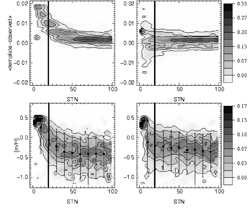
with $\sigma_{\mathrm{STN}}=16$, from the top left panel of Figure 2, reduces significantly the continuum normalization problem. The top panels in Figure 2 show the mean residual between the observed continuum-normalized spectra and best fit template as a function of S/N, before and after the change in the low rejection level, while the bottom panels present the resulting distributions of $\mathrm{[m/H]}$ as a function of S/N.

The new continuum normalization reduces significantly the correlation between metallicity and S/N, while no trend in the residual as a function of S/N remains. This indicates that the new continuum normalization algorithm performs adequately, although a weak correlation is still seen in the metallicity versus S/N ($\sim 0.1\,$dex per 100 in S/N).

Figure 2: Top panels: average residuals best fit template$-$observed spectra for 4,684 RAVE spectra as a function of S/N. Bottom panels: $\mathrm{[m/H]}$ distributions as a function of S/N. The left columns are for the previous version of the continuum normalization algorithm while the right column includes the low rejection level being a function of S/N. The gain from the new continuum normalization is clear from these figures: the correlation between metallicity and S/N is strongly reduced, while the residuals do not show any correlation with S/N. The thick black line represents the STN limit below which atmospheric parameters are not published in the RAVE catalog.

2.4 Masking bad pixels

Approximately 20% of RAVE spectra suffer from defects such as fringing or residual cosmic rays, which cannot be removed by the automatic procedure we use to reduce our data. While residual cosmic rays do not affect the determination of the stellar atmospheric parameters (these are similar to emission lines, which are not taken into account in the template library), fringing results in poor local continuum normalization, leading to inaccurate parameter recovery.

Regions strongly affected by fringing are difficult to detect prior to the processing, but we can make use of the best fit template to estimate whether a spectrum suffers from such a continuum distortion and therefore whether the atmospheric parameter determination is likely to be in error.

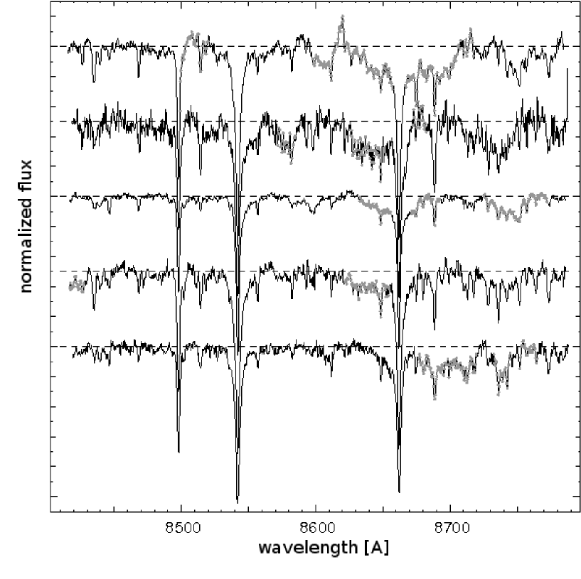
To estimate the fraction of a spectrum contaminated by continuum distortions, we compute the reduced $\chi^{2}(i)$ along the spectrum in a box 21 pixels wide centered on the pixel $i$. We then also compute the mean difference $S(i)$ between the best-fit template and the observed spectrum in the same box. If $\chi^{2}(i)>2$ and $S(i)>2/\mathrm{STN}$, a systematic difference between the template and the observed spectrum exists. The corresponding region of the spectrum is then flagged as a defect. The fraction of good pixels in each spectrum is then recorded and given in the RAVE catalog (see MaskFlag in Table 12). From visual inspection, we find that when the number of bad pixels is larger than 30% then the spectrum is problematic and the stellar parameters should be treated with caution. Figure 3 shows different examples of real RAVE spectra where a significant fraction of the spectrum is marked as defect.

Figure 3: Example of five RAVE spectra with regions marked as problematic by the MASK code. The regions marked in grey are recognized as suffering from poor continuum normalization. If more than 30% of the spectrum is marked by the code, the observation is flagged as problematic by the pipeline. The normalized fluxes are in arbitrary units and a vertical offset is added between the spectra for clarity.

2.5 Improving the zero-point correction

As explained in previous papers (e.g., Paper I), thermal instabilities in the spectrograph room induce zero point shifts of the wavelength solution that depend on the position along the CCD (e.g., fiber number). This results in instabilities of the radial velocity zero-point.

To correct the final radial velocities for this effect, the processing pipeline uses available sky lines in the RAVE window and fits a low-order polynomial ($3^{\rm rd}$ order) to the relation between sky radial velocity and fiber number. This $3^{\rm rd}$ order polynomial defines the mean trend of zero point offsets and provides the zero point correction as a function of fiber number. However, in some cases, a low-order polynomial is not the best solution and a constant shift should be used instead. In former releases, these cases were corrected by hand in the catalog. In this release, we introduced a new zero-point correction routine to the processing pipeline that is able to select which correction should be applied, automatically.

The zero-point correction now computes both the cubic correction, using the $3^{\rm rd}$ order polynomial, and the constant correction. It then computes the mean and standard deviation between the measured sky radial velocities and the corrections for the entire field and for three regions in fiber number that are contiguous on the CCD (fibers 1$-$50, 51$-$100, 101$-$150). For each region, the cubic fit is used unless any of these four conditions apply:

• there are less than two sky fibers in that region, to avoid under-constrained fits,

• the mean in that region for the constant correction is better than the corresponding mean for the cubic fit,

• the standard deviation for the cubic correction is greater than $5\,\rm{km\,s}^{-1}$, which is the case for noisy data,

• the maximum difference between the constant correction and the cubic correction is larger than $7\,\rm{km\,s}^{-1}$.

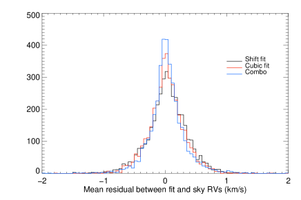
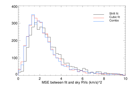
We tested the new procedure, together with other options, against pairs of repeat observations. The results are presented in Table 1. They show clearly that the new procedure performs better than the previous version in terms of dispersion, while the mean difference is unchanged. While the constant term correction appears better in this table, the left panel in Fig. 4 shows that the distribution of the residuals is less peaked than for the cubic correction. In addition, the mean-square-error, defined as $MSE=E[(RV-RV_{\rm fit})^{2}]$, shows a net decrease with the new fitting procedure compared to a constant shift. This indicates that for the general case, a constant correction for the entire field will result in a larger dispersion and hence a larger zero-point offset residual. This gives us confidence in the use of the new procedure.

Figure 4: Left: mean residual between the fit and the sky radial velocity for three different fitting functions. A constant shift (black histogram), the cubic fit used in DR1 and DR2 (red histogram), and the new fitting procedure (blue histogram). Right: associated mean-square-error.

Table 1: Radial velocity difference between pairs of repeat observations using different zero-point correction solutions. The old correction is a combination of cubic fit and corrections applied by hand. The number of pairs used is 25,172.

Method	$\mu~{}(\!\,\rm{km\,s}^{-1})$	$\sigma~{}(\!\,\rm{km\,s}^{-1})$	$N_{\rm reject}$	68% ($\!\,\rm{km\,s}^{-1}$)	95% ($\,\,\rm{km\,s}^{-1}$)
No correction	0.38	2.74	2 572	3.0	18.9
Old correction	0.23	2.49	2 765	2.8	16.8
Cubic	0.22	2.52	2 958	2.9	21.3
Quadratic	-0.44	2.83	2 645	3.2	20.2
Linear	0.24	2.21	2 850	2.5	16.7
Constant	0.23	2.05	2 990	2.3	16.5
New correction	0.23	2.22	2 817	2.5	16.6

3 Calibration and validation

3.1 Radial velocity

3.1.1 Internal error distribution

RAVE obtains its radial velocity from a standard cross-correlation routine. For each radial velocity measurement the associated error, eRV, gives the internal error due to the fitting procedure. Figure 5 presents the distribution of eRV per $0.2\,\rm{km\,s}^{-1}$ bin for the data new to each RAVE release. While first year data are of lower quality due to the second-order contamination of our spectra, second and third year data are of equal quality with a mode at $0.8\,\rm{km\,s}^{-1}$, a median radial velocity error of $1.2\,\rm{km\,s}^{-1}$, and 95% of the sample having internal errors better than $5\,\rm{km\,s}^{-1}$. Comparing these values to the old version of the pipeline used for DR1 and DR2 (see Table 2 and Fig. 9 of Paper II), the new pipeline marginally improves the internal accuracy with a gain of $\sim 0.1\,\rm{km\,s}^{-1}$ for the mode and the median radial velocity error.

Figure 5: Distribution of the radial velocity error (eRV) in the 3^rd data release. Top: number of stars with eRV in $0.2\,\rm{km\,s}^{-1}$ bins for first-year data (dash-dotted line), second-year data (dashed line), and third-year data (full line). Bottom: cumulative distribution of the eRV. The dotted lines mark respectively 50, 68 and 95% of the samples.

The aforementioned error values represent the contribution of the internal errors to the RAVE error budget. External errors are also present and are partially due to the zero-point correction which corrects only a mean trend, not including the fiber-to-fiber variations. The contribution of the external errors is obtained using external datasets and is discussed in Section 3.1.3.

3.1.2 Zero-point error

Our internal error budget is the sum of (i) the error associated with the evaluation of the maximum of the Tonry-Davis correlation function, and (ii) the contribution from the zero-point error. The first contribution is given by the pipeline (§ 3.1.1). The magnitude of the second term can be obtained from the analysis of the re-observed targets as, for a given star whose apparent magnitude is fixed, the radial velocity is constant (if the star is not a binary) and the internal errors are the main source of uncertainties.

We therefore use the re-observed stars in the RAVE DR3 catalog, selecting only stars observed during the second and third year, as they share the same global properties in terms of observing conditions. Data from the first year of observing are discarded, as they suffer from second-order contamination which renders the internal error inhomogeneous and can therefore bias our estimate. We also removed from the sample stars that were observed on purpose to calibrate our stellar atmospheric parameters, as these are specific bright targets with high S/N that do not share the random selection function nor the standard observational protocol of the RAVE catalogue.

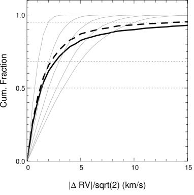
The cumulative distribution of the radial velocity difference is presented in the left panel of Fig. 6 where the solid line represents the full sample of re-observed targets and the dashed line the sample restricted to individual measurements differing by less than $3\sigma$ in a pair. Since our sample is contaminated by spectroscopic binaries, this selection is compulsory if one wants to address the error distribution for normal stars but is only a crude approximation when trying to remove all the binaries in the sample. Applying this cut rejects 6% of the sample, a value clearly below the expected contamination (see below). Therefore, the errors estimated from the repeat observations are likely to overestimate the true errors. With this limitation in mind, from Fig. 6, focusing on the dashed line, one can conclude that 68.2% of the sample has an error below $2.2\,\rm{km\,s}^{-1}$ while $\sim 93$% of the sample lies below the $5\,\rm{km\,s}^{-1}$ accuracy limit.

To estimate the contribution from the zero-point errors to the total internal error budget, we computed the distribution of the normalized radial velocity difference, the relative difference in radial velocity between two observations divided by the square root of the quadratic sum of the errors on radial velocity. If our measurements were affected only by the random errors for (i), then the distribution of this normalized radial velocity difference would follow a Gaussian distribution of zero mean and unit standard deviation. An additional contribution to the error budget due to a random zero-point error would broaden the distribution and hence enhance the dispersion of the resulting distribution. The result of this test is presented in the right panel of Figure 6, where we fitted the sum of two Gaussians to the observed distribution.

Figure 6: Left: Cumulative fraction of the radial velocity difference for re-observed RAVE targets in the Third Data Release. The solid line corresponds to the full sample, and the dashed line relates to the sample restricted to pairs whose individual measurement differ by less than 3$\sigma$ (hence rejecting the spectroscopic binaries with the largest radial velocity difference). The horizontal lines indicate 50, 68.2, and 95% of the sample. The grey lines are the expected distributions of the radial velocity difference for Gaussian errors of 1, 2, 3, 4, and $5\,\rm{km\,s}^{-1}$ from inside out. Right: distribution of the radial velocity difference $\Delta RV$ in units of $\sigma$ for re-observed targets. The blue line corresponds to our best-fit double Gaussian model to the distribution. The red dashed lines show the respective contribution of each Gaussian.

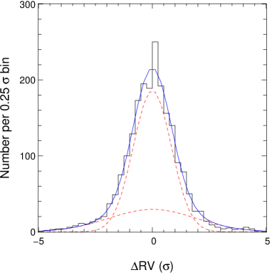
The dominant Gaussian distribution corresponds to stars stable in radial velocity. The width of the associated Gaussian function is $0.83\sigma$, narrower than a normal distribution, indicating that the internal errors quoted in the catalog are likely overestimated. Our quoted internal error can therefore be assumed to be an upper bound on the true internal errors, including the contribution of the zero-point error.

Spectroscopic binary contamination: subsidiarily, the broad Gaussian comprises spectra with defects (or where the zero-point solution could have diverged) as well as the contribution from spectroscopic binaries. The fraction of spectra with defects is small in this sample, as the catalog has been cleaned of fields where the zero-point solution did not converge. Hence, the relative weight of the two Gaussian functions gives an estimate, in reality an upper limit, of the contamination level by spectroscopic binaries with radial velocity variation between observations larger than $1\sigma$ in the RAVE catalog. Our best-fit solution gives a relative contribution for this second population of 26% which allows us to conclude that the fraction of spectroscopic binaries with radial velocity variations larger than $2\,\rm{km\,s}^{-1}$ in the RAVE catalog is less than or equal to 26%. A more detailed analysis of repeated observations based on 20 000 RAVE stars by Matijevič et al. (2011) gives a lower limit of 10-15% of the RAVE sample being affected by binarity (see also Matijevič et al., 2010). However, the time span between repeat observations being biased towards short periods (days to weeks), long period variations are not detected. The previous estimates do not take into account this population and a more detailed analysis will be required to estimate the contribution of long period variables to our survey.

3.1.3 Validation using external datasets

Our external datasets (or, ‘reference’ datasets) comprise data from the Geneva-Copenhagen Survey (Nordström et al., 2004, hereafter GCS), Elodie and Sophie high resolution observations from the Observatoire de Haute Provence, Asiago echelle observations, and spectra obtained with the ANU 2.3m facility in Siding Spring. The targeted stars are chosen to cover the possible range of signal-to-noise conditions and stellar atmospheric conditions. Figure 7 presents the distributions of the reference stars as a function of signal-to-noise S2N, ${T_{\rm eff}}$ $\log g$ and $\mathrm{[m/H]}$ compared the the RAVE DR3 distributions. While for $\mathrm{[m/H]}$ the distribution ressembles the distribution of the data release, the distribution of $\log g$ shows a lack of giant stars that translates to a reduced peak at temperature below $5\,000$ K compared to the full DR3 sample. This is due to the GCS sample, our primary source of reference stars, that contains F and G dwarfs and no giants. For the S2N distribution, we chose to sample almost uniformly the RAVE S2N interval, top left panel of Fig. 7, which enables us to verify that signal-to-noise does not impact the quality of our radial velocities (see below).

Figure 7: Histograms of the distribution of the reference sample (dash-dotted histograms) and the RAVE DR3 sample (full lines) as a function of signal-to-noise, ${T_{\rm eff}}$, $\log g$ and RAVE $\mathrm{[m/H]}$. The dash-dotted histograms are multiplied by a factor 50 to enhance their visibility.

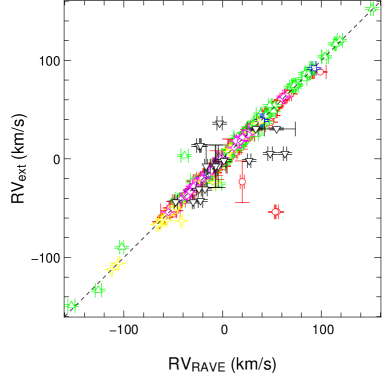
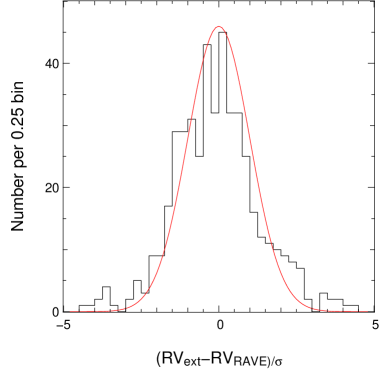
A comparison of the radial velocities obtained by RAVE and the external datasets is presented in Figure 8, while the detailed values for the comparison for each sample can be found in Table 2.

Figure 8: Comparison of RAVE radial velocities to external sources. Left : $RV_{\rm RAVE}$ vs. $RV_{\rm ext}$ for all the different sources: GCS (red circles), ANU 2.3m (green triangles), Elodie (blue squares), Sophie (yellow crosses), and Asiago echelle spectra (magenta diamonds). The black downwards triangles are stars identified as binaries. Right: distribution of the radial velocity differences divided by the associated errors. The red curve is a Gaussian distribution with zero mean and $\sigma=1$.

Table 2: Global properties of the comparison of RAVE radial velocities to external datasets for stars observed during the second and third year of the program. $\Delta RV$ is defined as $\Delta RV=RV_{\rm ext}-RV_{\rm RAVE}$. The mean deviations and standard deviations are computed using a sigma clipping algorithm. The second column gives the number of data points used to compute the mean and $\sigma$ while the numbers in parenthesis are the total number of stars in the sample ($N_{1}$) and the number of unique objects ($N_{2}$). The last two lines are obtained after correcting each dataset for the mean deviation.

Reference	$N$	($N_{1}$,$N_{2}$)	$\langle\Delta RV\rangle$	$\sigma(\Delta RV)$
dataset			$\!\,\rm{km\,s}^{-1}$	$\!\,\rm{km\,s}^{-1}$
GCS	224	(285,162)	-0.28	1.76
Sophie	35	(37,34)	-0.77	1.62
Asiago	30	(30,25)	1.08	1.45
Elodie	6	(9,9)	-0.63	0.36
2.3m	76	(125,74)	0.87	2.39
All	373	(486,304)	-0.22	2.72
All but GCS	142	(201,142)	0.50	2.16
mean deviation corrected
All	142	(486,304)	-0.18	2.66
All but GCS	127	(201,142)	0.10	1.96

With the new version of the pipeline, we find no significant difference for the mean radial velocity difference compared to DR2. The values for the mean difference and its dispersion are consistent between these two releases. From the right panel of Figure 8 one sees that the distribution of the radial velocity difference divided by the internal errors is wider than a normal distribution : its dispersion is 1.37$\sigma$. We can then estimate the upper limit to the external error contribution as $\sigma_{\rm ext}\leq 0.9\,\rm{km\,s}^{-1}$. This is an upper limit as the zero-point errors of the other sources of radial velocity also contribute to the measured $\sigma_{\rm ext}$ and are unknown.

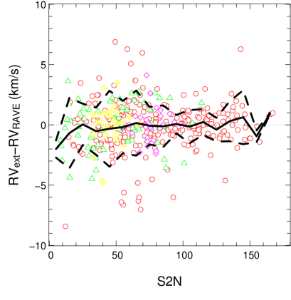
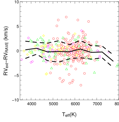
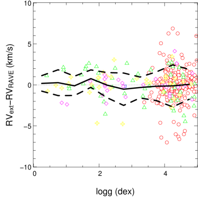
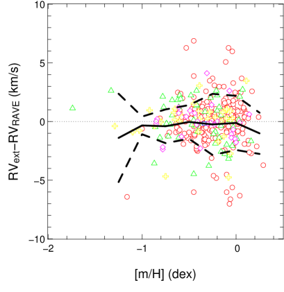
The dependency of the radial velocity difference on signal-to-noise ratio is weak, as can be seen from Figure 9 (top left panel). The mean difference is consistent with no offset, at all S2N levels. There is a slight tendency for an increase in dispersion at low S2N, but the dispersion values remain very well-behaved ($\sigma\sim 1.2\,\rm{km\,s}^{-1}$ at S2N$>$100 and $\sigma\sim 2.0\,\rm{km\,s}^{-1}$ for S2N$<$40). In addition, no strong variation with $\log g$, ${T_{\rm eff}}$, or $\mathrm{[m/H]}$ is seen, indicating that our radial velocity solution is stable as a function of stellar type.

Figure 9: Radial velocity difference between the RAVE observations and the external sources as a function of the signal-to-noise ratio S2N (top left), effective temperature (top right), $\log g$ (bottom left), and $\mathrm{[m/H]}$ (bottom right) of the RAVE observation. The symbols follow Figure 8 while the full and dashed thick lines represent the mean and dispersion about the mean of the radial velocity difference per interval of 10 in S2N, 500 K in ${T_{\rm eff}}$, 0.5 dex in $\log g$, or 0.25 dex in $\mathrm{[m/H]}$.

3.2 Stellar atmospheric parameters

During the second and third years of its program, RAVE observed $2\,266$ stars more than once; $1\,917$ stars were observed twice, $256$ were observed three times, and $93$ were observed four times. $1\,391$ of these stars have more than one measurement of stellar parameters. We use these re-observations to estimate the stability and error budget for our estimated stellar atmospheric parameters. These parameters are the parameters from the synthetic template spectrum used to compute the final radial velocity. This template is constructed using a penalized chi-square algorithm where the template spectrum is a weighted sum of the synthetic spectra of the library of Munari et al. (2005). The weights of the best-match are obtained by minimization of a $\chi^{2}$ plus additional constraints (weights must be positive and smoothly distributed in the atmospheric parameters space). The algorithm is described in Paper II.

3.2.1 Internal stability from repeat observations

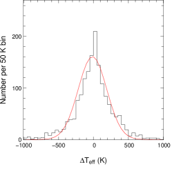
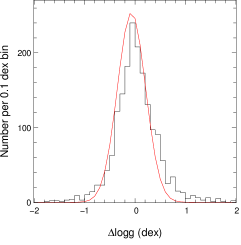
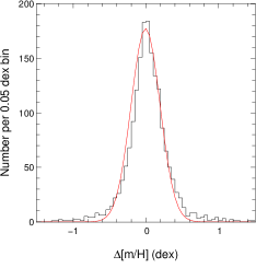
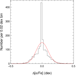
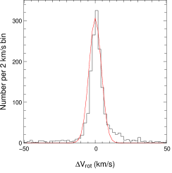
As a first step, we estimate the stability from the difference in the measured parameters using, for a given star, the spectrum with the highest S/N  as the reference measurement. The distribution of the stellar parameter differences $\Delta P$, where $P$ may stand for any of the stellar atmospheric parameters considered, is shown in Figure 10 while Figure 11 presents the distributions for dwarfs and giants stars respectively. The red curves in each panel are Gaussian functions whose parameters (mean and standard deviation) are obtained using an iterative sigma-clipping algorithm. The corresponding mean and standard deviation for each parameter are reported in Table 3. For all parameters, the mode of the distributions is consistent with zero, indicating good stability of our atmospheric parameter measurements. The average internal error for the atmospheric parameters can be estimated from the standard deviation. For ${T_{\rm eff}}$ one obtains 200 K and 0.3 dex for $\log g$, while the $\mathrm{[m/H]}$ and $\mathrm{[\alpha/Fe]}$ distributions show a dispersion of 0.2 and 0.1 dex respectively. These values must be regarded as underestimates of the true errors as they do not include external errors such as the inadequacy of the template library in representing real spectra or variations in the abundances of the chemical species with respect to the solar abundances (using but one value of the $\alpha$-enhancement).

In Fig. 10 the distributions of ${T_{\rm eff}}$, $\mathrm{[m/H]}$ and $\mathrm{[\alpha/Fe]}$ are relatively symmetric although not Gaussian. The distribution of $\log g$ is less symmetric and that of ${V_{\rm rot}}$ is very skew. Since our reference measurements are the spectra with the highest S/N, symmetry indicates that there is no strong bias in the atmospheric parameter estimation as one reduces the signal-to-noise ratio: a systematic effect with the S/N would imply that as one lowers the S/N the measured parameters would be either higher or lower than the reference value.

For ${V_{\rm rot}}$, a systematic effect is likely. As one lowers the S/N, the wings of the spectral lines become more affected by the noise, making the lines appear narrower, hence mimicking a lower ${V_{\rm rot}}$. The same effect applies to $\log g$.

Figure 10: Distributions of the difference in the measured stellar atmospheric parameters in re-observed targets. The spectrum with highest S/N for a given star is used as reference. The red lines in the different panels correspond to a Gaussian function whose parameters (mean and dispersion) are obtained using an iterative sigma-clipping algorithm (see Table 3).

Figure 11: Same as Fig. 10 but for the sub-samples of dwarf stars (top curves) and giant stars (bottom curves). The samples are selected according to $\log g$ using the separating line $\log g=3.5$ dex. The histograms for dwarf stars are shifted upwards by 100 counts per bin for clarity.

Table 3: Standard RAVE errors on stellar atmospheric parameters from repeat observations for the full sample of re-observed stars. The mean and standard deviations are computed using an iterative sigma-clipping algorithm and $\Delta P=P_{\rm ref}-P_{\rm star}$.

$P$		$\langle\Delta P\rangle$	$\sigma_{P}$
${T_{\rm eff}}$	(K)	-7	204
$\log g$	(dex)	0.0	0.3
$\mathrm{[m/H]}$	(dex)	0.0	0.2
$\mathrm{[\alpha/Fe]}$	(dex)	0.0	0.1
${V_{\rm rot}}$	($\,\,\rm{km\,s}^{-1}$)	0.3	4.3

Internal errors on the atmospheric parameters depend on the physical condition of the star, $\log g$ being better constrained for giants and ${T_{\rm eff}}$ for cool stars. The internal errors, as defined in Paper II, depend mostly on the algorithm used and the grid spacing of the synthetic spectra for these two parameters. Neither has been modified in the new version of the pipeline. Hence, the internal errors for the different parameters remain unchanged and upper limits for these errors are presented in Fig. 19 in Paper II. However, using re-observed RAVE stars, one is able to refine this estimate based on the scatter of the atmospheric parameter measurements in various ${T_{\rm eff}}$ and $\log g$ intervals. These refined estimates are presented in Table 4 where a smooth-averaging procedure is used to compute the dispersion at a given grid point. Only grid points with three or more repeated observations are given in the table.

Table 4: Dispersion in ${T_{\rm eff}}$ (K), $\log g$ (dex) and $\mathrm{[m/H]}$ (dex) as a function of ${T_{\rm eff}}$ and $\log g$. The dispersions are computed by smooth-averaging sigmas in individual grid points. Only grid points where three or more repeated objects are present are quoted.

${T_{\rm eff}}$(K)$\backslash\log g$ (dex)		0	0.5	1	1.5	2	2.5	3	3.5	4	4.5	5
	(${T_{\rm eff}}$)	30	40	50	50	80	180	500	200	100	100	110
4000	($\log g$)	0.07	0.16	0.19	0.21	0.43	0.29	0.81	0.62	0.17	0.16	0.051
	($\mathrm{[m/H]}$)	0.06	0.08	0.08	0.09	0.14	0.42	0.13	0.26	0.10	0.07	0.11
	(${T_{\rm eff}}$)		50	60	60	50	50	60	160	120	70	50
4500	($\log g$)		0.12	0.18	0.20	0.18	0.19	0.22	0.34	0.16	0.17	0.06
	($\mathrm{[m/H]}$)		0.07	0.09	0.08	0.07	0.07	0.08	0.09	0.09	0.09	0.06
	(${T_{\rm eff}}$)				180	70	70	90	110	100	80	50
5000	($\log g$)				0.58	0.17	0.21	0.24	0.20	0.16	0.14	0.06
	($\mathrm{[m/H]}$)				0.28	0.07	0.09	0.09	0.09	0.08	0.07	0.05
	(${T_{\rm eff}}$)					600	200	180	190	130	120	90
5500	($\log g$)					0.39	0.29	0.38	0.27	0.14	0.12	0.08
	($\mathrm{[m/H]}$)					0.13	0.17	0.17	0.12	0.10	0.08	0.05
	(${T_{\rm eff}}$)						850	300	180	110	120	100
6000	($\log g$)						0.98	0.89	0.28	0.15	0.14	0.08
	($\mathrm{[m/H]}$)						0.36	0.43	0.11	0.10	0.09	0.07
	(${T_{\rm eff}}$)							400	140	110	130	130
6500	($\log g$)							1.13	0.18	0.14	0.16	0.08
	($\mathrm{[m/H]}$)							0.35	0.13	0.10	0.10	0.08
	(${T_{\rm eff}}$)								160	150	150	140
7000	($\log g$)								0.13	0.12	0.17	0.07
	($\mathrm{[m/H]}$)								0.08	0.10	0.12	0.12
	(${T_{\rm eff}}$)								200	110	200	500
7500	($\log g$)								0.16	0.10	0.15	0.19
	($\mathrm{[m/H]}$)								0.11	0.08	0.11	0.21

3.2.2 Effect of the correlations between atmospheric parameters

In Paper II, we showed that the method we use to estimate the stellar atmospheric parameters introduces correlations in the errors of the recovered parameters. Here, we use the re-observations of standard RAVE program stars to estimate the amplitude of these correlations. The results of these tests are presented in Figure 12 where the contours in each panel contain 30, 50, 70, and 90% of the total sample. Looking at the different panels, a clear correlation is observed between the deviations in ${T_{\rm eff}}$, $\log g$ ,and $\mathrm{[m/H]}$ while deviations in $\mathrm{[\alpha/Fe]}$ are only correlated with deviations in $\mathrm{[m/H]}$. ${V_{\rm rot}}$ on the other hand does not show any correlation, regardless of the atmospheric parameter considered. Since the correlation between $\log g$ and $\mathrm{[m/H]}$ is broader than between $\log g$ and ${T_{\rm eff}}$, it is likely that errors on ${T_{\rm eff}}$ are the primary source of errors, and that these errors propagate to the other atmospheric parameters.

These correlations indicate that the true $\mathrm{[M/H]}$ will be a function of all the parameters, except for ${V_{\rm rot}}$. The correlation with $\log g$ being weaker than that with ${T_{\rm eff}}$ and $\mathrm{[m/H]}$, the true calibration relation might be independent of $\log g$ or at least, we expect $\log g$ to play a secondary role in the estimation of the true $\mathrm{[M/H]}$. This will be studied more deeply in the next paragraph.

	$\Delta{T_{\rm eff}}$ (K)	$\Delta\log g$ (dex)	$\Delta\mathrm{[m/H]}$ (dex)	$\Delta\mathrm{[\alpha/Fe]}$ (dex)
$\Delta V_{\rm rot}\ (\,\rm{km\,s}^{-1})$
$\Delta\mathrm{[\alpha/Fe]}$ (dex)
$\Delta\mathrm{[m/H]}$ (dex)
$\Delta\log g$ (dex)

Figure 12: Correlation between the stellar atmospheric parameters based on re-observed RAVE targets. The contours contain 30, 50, 70, and 90% of the data respectively. A correlation between the error in two parameters indicates that a systematic error in one parameter influences the result in the other.

3.2.3 Comparison to external data

In the previous paragraphs, we checked the consistency of the RAVE atmospheric-parameter solutions and the correlations that exist between these parameters. The consistency of the atmospheric parameters is satisfactory given our medium resolution ($R\sim 7\,500$) and our small wavelength interval. The dispersions around the reference values are $\sim 200$ K for ${T_{\rm eff}}$, 0.3 dex for $\log g$, 0.2 dex for $\mathrm{[m/H]}$, and 0.1 dex for $\mathrm{[\alpha/Fe]}$, with no significant centroid offset.

The next step is to compare our measured atmospheric parameters with independent measurements. As for DR2, RAVE stars are generally too faint to have been observed in other studies from the literature. We therefore used custom RAVE observations of bright stars from the literature as well as high-resolution observations of bright RAVE targets to construct our calibration sample. This sample comprises four different sources of atmospheric parameters:

• RAVE observations of Soubiran & Girard (2005) stars,

• Asiago echelle observations of RAVE targets ($R\sim 20\,000$),

• AAT 3.9m UCLES echelle observations of RAVE targets,

• APO ARC echelle observations of RAVE targets ($R\sim 35\,000$).

The last three sources of calibration data make the bright RAVE targets sample and were all reduced and processed within the RAVE collaboration using the same technique and are therefore merged in the following and referred to as “echelle data”. We follow a standard analysis procedure using Castelli ODFNEW atmosphere models. The gf values for iron lines are taken from three different sources

• the list from Fulbright (2000) for metal poor stars based

• a list of differential $\log gf$ from Acturus (Fulbright et al., 2006) best suited for metal rich giants

• a list of differential $\log gf$ from the Sun best suited for dwarf stars.

The three line lists give reasonable agreement ($\Delta{T_{\rm eff}}<50\,{\mathrm{K}}$ and $\Delta\mathrm{[Fe/H]}<0.1\,{\mathrm{d}ex}$) in the parameter boundary regions. The alpha- and heavy-element line list is basedon Fulbright (2000) for metal-poor stars and Fulbright et al. (2007) for metal-rich stars. ${T_{\rm eff}}$ values are obtained using the excitation balance, forcing the distribution of $\log\epsilon({\mathrm{F}e})$ vs. excitation potential for individual Fe I lines to have a flat slope. $\log g$ is obtained via the ionisation balance, forcing the $\log\epsilon(\mathrm{Fe})$ values derived from Fe I and Fe II lines to agree. Both methods are fully independent from the technique used by the RAVE pipeline to estimate atmospheric parameters from medium-resolution spectra.

For the RAVE observation of stars studied in the literature, we chosed to build our sample upon the Soubiran & Girard (2005) catalog. This catalog contains abundances measurements from the literature paying a particular attention at reducing the systematics between the various studies. It makes this catalog particularly suited for calibration purposes.

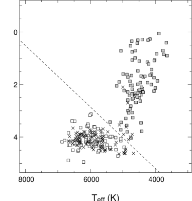
Table 5 summarizes the content of each sample while Figure 13 presents the distribution in $\log g$ and ${T_{\rm eff}}$ of stars in the calibration sample. The GCS also provides photometric ${T_{\rm eff}}$ measurements but as for DR2, we choose not to include photometric ${T_{\rm eff}}$ in our analysis.

Figure 13: Location of the reference stars in the (${T_{\rm eff}}$,$\log g$) plane. Squares are echelle data, the dashed line representing our separation between dwarfs (open symbols) and giants (grey symbols) for the calibration relation. Crosses are stars in Soubiran & Girard (2005).

Table 5: Samples used to calibrate the RAVE atmospheric parameters. The echelle sample covers the data obtained using UCLES, ARC, and Asiago spectrographs and were processed and analysed consistently.

Sample	$N_{\rm star}$	$N_{\rm obs}$	${T_{\rm eff}}$	$\log g$	$\mathrm{[M/H]}$	$\mathrm{[\alpha/Fe]}$
Echelle	162	228	$\surd$	$\surd$	$\surd$	$\surd$
Soubiran & Girard	102	107	$\surd$	$\surd$	$\surd^{(1)}$	$\surd$
(1): Soubiran & Girard (2005) do not report metallicity $\mathrm{[M/H]}$, so their values are derived from a weighted sum of the quoted element abundances of Fe, O, Na, Mg, Al, Si, Ca, Ti, and Ni, assuming the solar abundance ratio from Anders & Grevesse (1989).

In the following, we separate the analysis of ${T_{\rm eff}}$ and $\log g$ from $\mathrm{[M/H]}$, the latter requiring a specific calibration.

$\bullet$ ${T_{\rm eff}}$ and $\log g$ :

Table 6 presents the results of the comparison of the RAVE pipeline outputs with the reference datasets. Since outliers are present, we use a standard iterative (sigma-clipping) procedure to estimate the mean offset and standard deviation for each atmospheric parameter. The new version of the pipeline shows a slight tendency to overestimate ${T_{\rm eff}}$ by $\sim 50-60$ K compared to the previous version, with an increase of the standard deviation from 188 K to 250 K. For $\log g$ the results are consistent between the two versions of the pipeline. We note here that the reference samples used for the new release have increased considerably, with the number of Soubiran & Girard (2005) stars increasing by a factor of two and the number of echelle observations by a factor of four.

Table 6: Mean offset and standard deviation for ${T_{\rm eff}}$ and $\log g$ between the reference datasets and RAVE DR3 values. $N_{\rm tot}$ is the total number of observations in the reference datasets, and $N_{\rm rej,Teff}$ and $N_{\rm rej,\log g}$ are the number of observations rejected by the iterative procedure for estimating the mean difference and dispersion for ${T_{\rm eff}}$ and $\log g$ respectively.

Sample	$N_{\rm tot}$	$\Delta{T_{\rm eff}}$	$\sigma_{T_{\rm eff}}$	$N_{\rm rej,Teff}$	$\Delta\log g$	$\sigma_{\log g}$	$N_{\rm rej,\log g}$
Echelle	227	$-85\pm 14$	209	11	$-0.12\pm 0.03$	0.43	6
Soubiran & Girard	107	$-63\pm 26$	262	7	$-0.05\pm 0.03$	0.35	2
All	334	$-72\pm 14$	251	12	$-0.10\pm 0.02$	0.40	9

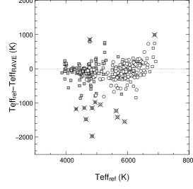
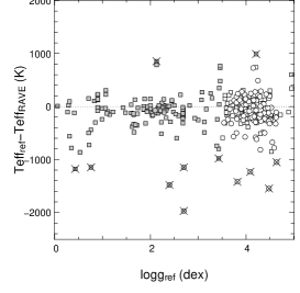
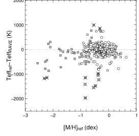
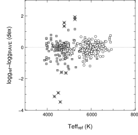
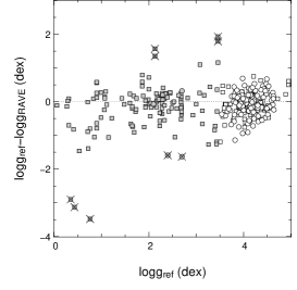
To further validate our atmospheric parameters, we compare the offset between the reference atmospheric parameters with the RAVE values. This is presented in Figure 14 for ${T_{\rm eff}}$ (top panels) and $\log g$ (bottom panels) as a function of reference ${T_{\rm eff}}$ (left), $\log g$ (middle), and $\mathrm{[m/H]}$ (right). The crosses indicate the data discarded by the iterative procedure as being outliers.

For ${T_{\rm eff}}$, no correlation is observed either as a function of ${T_{\rm eff}}$ or $\mathrm{[m/H]}$. Considering the echelle data alone (open squares) a tendency for ${T_{\rm eff}}$ to be overestimated as $\log g$ increases is observed, producing the $-85\,$K offset reported in Table 6. However, at low $\log g$ the discrepancy vanishes. This tendency is not seen for the Soubiran & Girard (2005) stars. Since this effect is not systematic, it leads us to conclude that the apparent trend in ${T_{\rm eff}}$ with $\log g$ is not due to the RAVE data but instead due to the different methods used to derive this parameter in the other works.

For $\log g$, no trend is observed with ${T_{\rm eff}}$. However a trend with $\log g$ seems to be present, such that the RAVE $\log g$ is slightly overestimated at the low end (by $\sim$0.5 dex). In addition, a tendency to overestimate $\log g$ at low metallicities is seen, amounting to the same order. Because this effect is limited to the very low $\log g$ end of the distribution ($\log g<1$), which is not highly populated in the RAVE catalog, this leads to the conclusion that our $\log g$ determination are reliable within our quoted uncertainties.

Figure 14: Difference between the atmospheric parameters of the reference datasets and of the RAVE DR3 parameters as a function of the reference ${T_{\rm eff}}$, $\log g$ and $\mathrm{[M/H]}$ for ${T_{\rm eff}}$ (top), and $\log g$ (bottom). Circles stand for stars in Soubiran & Girard (2005) while squares denote echelle data. Grey symbols represent the giants, open symbols mark the location of the dwarfs. Crosses indicate data rejected by the iterative procedure used for Table 6.

$\bullet$ $\mathrm{[M/H]}$ :

As stated in Paper II, the metallicity indicator obtained by the RAVE pipeline is, due to our medium resolution and limited signal-to-noise ratio, a mixture of the real metallicity, alpha enhancement, and possibly rotational velocity. To obtain an unbiased estimator, we rely on a calibration relation set using a sample of stars with known atmospheric parameters. Paper II presented a first calibration relation using an iterative fitting procedure of the relation

$$\mathrm{[M/H]}=c_{0}+c_{1}.\mathrm{[m/H]}+c_{2}.\mathrm{[\alpha/Fe]}+c_{3}.\log g\,.$$

The coefficients of this relation were obtained based on a sample of 45 APO, 24 Asiago, 49 Soubiran & Girard (2005), and 12 M67 cluster member stars. With the larger number of reference stars available for this release and due to the new version of the processing pipeline, modified to increase the reliability of the atmospheric parameters, we recompute and extend the calibration relation. However, we now restrict the analysis to the reference sample consisting of echelle data. This sample was selected to evenly cover the ($\log g$,${T_{\rm eff}}$) plane of the RAVE survey and was processed using the same technique and reduction algorithm, therefore providing an homogeneous set of reference data. Also, with the knowledge gained from the analysis of the correlation between parameters, the proposed calibration relation now takes the form

$$\mathrm{[M/H]}=c_{0}+c_{1}.\mathrm{[m/H]}+c_{2}.\mathrm{[\alpha/Fe]}+c_{3}.\frac{{T_{\rm eff}}}{5040}+c_{4}.\log g+c_{5}.\mathrm{STN}\,,$$ (2)

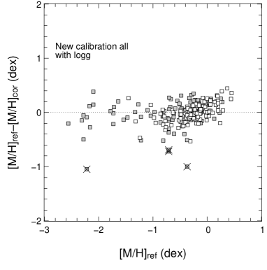
where we added ${T_{\rm eff}}$ to the calibration relation due to the strong correlation observed in Fig. 12 and discussed in Section 3.2.2. S/N is also included as one expects an impact of the noise at the low S/N regime where the pipeline may mistake noise spikes for enhanced metallicity. Since ${T_{\rm eff}}$ seems to be the primary source of error for $\mathrm{[m/H]}$, we computed four calibration relations for the various cases with and without S/N or $\log g$. As for the DR2 calibration, we see no evidence for higher order terms and therefore restrict our search for the best calibration to first order (linear) relations.

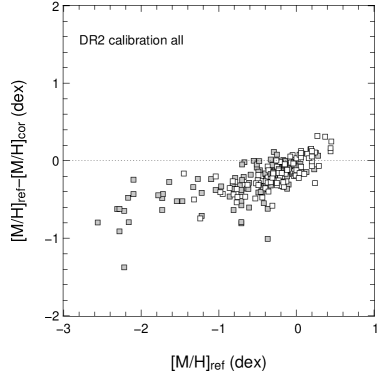
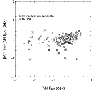
The coefficients for the calibration relations are obtained by minimizing the difference between the calibrated $\mathrm{[M/H]}$ and the reference $\mathrm{[M/H]}$ using an iterative procedure to reject outliers. The resulting calibration relations are summarized in Table 7 where $N_{\rm tot}$ is the total number of observations used to compute the calibration relation. A blank value in a column indicates that the calibration relation does not include the corresponding parameter. The residuals between the calibrated $\mathrm{[M/H]}$ and the reference $\mathrm{[M/H]}$ as a function of the reference $\mathrm{[M/H]}$ are presented in Figure 15 where the top panels present the raw output of the DR3 pipeline (panel marked original) and the residuals obtained using the DR2 calibration relation on the DR3 atmospheric parameters values. The following four panels are for the different calibration relations considered here. Finally, Table 8 presents the mean offset and standard deviation computed from the residuals in the different cases.

Table 7: Coefficients in the calibration relation for the RAVE metallicities using different sets of parameters for the fit. $N_{\rm tot}$ is the total number of data points used to derive the calibration, $c_{i}$ are the coefficients from Eq. 2. The first line presents the output of the new RAVE pipeline while the second line presents the results obtained when one applies the calibration relation of Paper II. The following lines are the calibration relations obtained using the new pipeline outputs.

Calibration	$N_{\rm tot}$	$c_{0}$	$c_{1}$	$c_{2}$	$c_{3}$	$c_{4}$	$c_{5}$
Full sample
DR2 calibration	-	0.404	0.938	0.767	-	-0.064	-
DR3 no S/N no $\log g$	223	$0.578\pm 0.098$	$1.095\pm 0.022$	$1.246\pm 0.143$	$-0.520\pm 0.089$	-	-
DR3 with S/N	217	$0.587\pm 0.091$	$1.106\pm 0.024$	$1.261\pm 0.140$	$-0.579\pm 0.078$	-	$0.001\pm 0.0004$
DR3 with $\log g$	223	$0.518\pm 0.127$	$1.111\pm 0.031$	$1.252\pm 0.144$	$-0.399\pm 0.187$	$-0.019\pm 0.026$	-
DR3 with S/N and $\log g$	222	$0.429\pm 0.132$	$1.101\pm 0.032$	$1.171\pm 0.147$	$-0.391\pm 0.186$	$-0.018\pm 0.026$	$0.001\pm 0.0004$
Dwarfs only
DR3 no S/N no $\log g$	89	$0.612\pm 0.236$	$1.081\pm 0.045$	$1.215\pm 0.203$	$-0.546\pm 0.196$	-	-
DR3 with S/N	75	$0.706\pm 0.199$	$1.250\pm 0.055$	$1.491\pm 0.184$	$-0.683\pm 0.165$	-	$0.001\pm 0.0004$
DR3 with $\log g$	82	$-0.174\pm 0.222$	$1.061\pm 0.047$	$1.621\pm 0.158$	$-0.751\pm 0.160$	$0.232\pm 0.038$	-
DR3 with S/N and $\log g$	81	$-0.170\pm 0.217$	$1.063\pm 0.047$	$1.586\pm 0.155$	$-0.751\pm 0.155$	$0.219\pm 0.037$	$0.001\pm 0.0003$
Giants only
DR3 no S/N no $\log g$	127	$0.763\pm 0.197$	$1.094\pm 0.027$	$1.210\pm 0.193$	$-0.711\pm 0.207$	-	-
DR3 with S/N	119	$0.399\pm 0.178$	$1.087\pm 0.027$	$1.300\pm 0.185$	$-0.383\pm 0.179$	-	$0.001\pm 0.0005$
DR3 with $\log g$	127	$0.354\pm 0.287$	$1.162\pm 0.044$	$1.285\pm 0.194$	$-0.049\pm 0.398$	$-0.078\pm 0.040$	-
DR3 with S/N and $\log g$	127	$0.239\pm 0.297$	$1.154\pm 0.045$	$1.217\pm 0.200$	$-0.006\pm 0.398$	$-0.080\pm 0.040$	$0.001\pm 0.0007$

Figure 15: Difference between the reference $\mathrm{[M/H]}$ and RAVE $\mathrm{[M/H]}$ using the different calibration relations as a function of reference $\mathrm{[M/H]}$. The crosses indicate the observations rejected from the fit by the iterative procedure.

Figure 16: Same as Fig. 15 but using separate calibration relations for dwarfs and giants.

Table 8: General properties of the different calibration relations presented in Tab. 7. $\Delta\mathrm{[M/H]}$ is the mean difference $\mathrm{[M/H]}_{\rm ref}-\mathrm{[M/H]}_{\rm corrected}$ and $\sigma_{\mathrm{[M/H]}}$ is the dispersion. $N_{\rm rej}$ is the number of observations rejected by the iterative procedure as outliers. For each calibration relation, we also provide separate statistics for dwarfs and giants obtained using the calibration relations derived specifically for each sample.

Calibration	$\Delta\mathrm{[M/H]}$	$\sigma_{\mathrm{[M/H]}}$	$N_{\rm rej}$
No calibration	0.10	0.24	-
DR2 calibration	-0.22	0.23	-
DR3 no SNR no $\log g$	+0.00	0.18	4
[-] Dwarfs	-0.01	0.14	7
[-] Giants	0.00	0.18	4
DR3 with SNR	0.00	0.16	10
[-] Dwarfs	0.01	0.10	21
[-] Giants	0.00	0.14	12
DR3 with $\log g$	0.00	0.18	4
[-] Dwarfs	0.00	0.10	14
[-] Giants	0.00	0.18	4
DR3 with SNR and $\log g$	0.00	0.17	5
[-] Dwarfs	0.00	0.10	15
[-] Giants	0.00	0.18	4

From Figure 15, it is clear that applying the DR2 calibration to the DR3 pipeline outputs is not satisfactory and produces a bias at low metallicity. This behavior is expected as the pipeline has been modified to produce a better agreement to the metallicity distribution which, for DR2 showed a reduced tail at the low metallicity end. As the correlation between the parameters is significant (see § 3.2.2) and because the calibration relation is built upon the output parameters (with a large contribution from $\mathrm{[m/H]}$ which is modified compared to the DR2 pipeline), one therefore expects the DR2 calibration relation not to hold for the DR3 parameters. Ideally, the DR3 parameters would not need a calibration relation. However the raw output of the DR3 pipeline still suffers from a small systematic effect, underestimating the true metallicity by $\sim$0.1 dex with some systematic dependency on ${T_{\rm eff}}$.

Applying the calibration relations proposed, the RAVE metallicties agree with the echelle values (see Table 8). However, as can be seen from Fig. 15, a systematic trend is observed for dwarfs at high metallicity, where the difference between RAVE and the echelle value reaches 0.4 dex for the highest metallicity stars. At low metallicity, the dispersion is significantly reduced and when applying any of the calibration relations, the two determinations agree well. Adding $\log g$ or S/N to the calibration relation does not improve the residuals significantly. For $\log g$ this is understood as it is the atmospheric parameter with the largest uncertainty. Hence its dispersion prevents it from having significant weight in the calibration relation, even though we know the error on this parameter is strongly correlated to errors in $\mathrm{[M/H]}$ (see Section 3.2.2). For S/N, the situation is less clear but part of its low weight in the calibration relation is linked to the fact that, in order to observe RAVE targets at high resolution, we selected targets in the bright part of the catalog to ensure enough S/N in the spectra to allow precise measurements of the atmospheric parameters. Hence, the region of the S/N space where this parameter plays an important role ($\hbox{S/N}<20$) is not properly sampled, lowering its weight on the calibration relation whereas above this threshold, no correlation with S/N is observed.

Finally, to improve on the situation for the dwarfs, we split the sample between dwarfs and giants (see Fig. 13 for the criterion used) and applied the same procedure to each sub-population. The result of these calibration relations is presented in Fig. 16, the basic statistics being reported in Table 8 for each calibration relation.

Using separate calibration relations for dwarfs and giants does help improve the dispersion for dwarfs, but, as we can see in Fig. 16, the calibration relation is unable to remove the bias at high $\mathrm{[M/H]}$, the most discrepant stars being rejected by the fit. Only a mild improvement is obtained. Separating the dwarfs from the giants changes the calibrated metallicity for these stars by only 0.02 dex, or 0.05 dex if one also uses $\log g$ in the calibration.

4 Catalog presentation

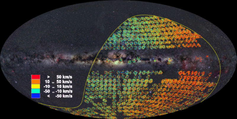
The DR3 release of the RAVE catalog contains $83\,072$ radial velocity measurements for $77\,461$ individual stars. Atmospheric parameters are provided for $41\,672$ spectra ($39\,833$ stars). These data were acquired over $257$ observing nights, spanning the time interval April $11^{\rm th}$ 2003 to March $12^{\rm th}$ 2006, and $976$ fields. The data new to this release cover the time interval March $31^{\rm st}$ 2005 to March $12^{\rm th}$ 2006 where $32\,477$ new spectra were collected. The total coverage of the pilot survey is then $11\,500$ square degrees. Figure 17 plots the general pattern of (heliocentric) radial velocities, where the dipole distribution is due to a combination of asymmetric drift and the Solar motion with respect to the Local Standard of Rest.

Figure 17: Aitoff projection in Galactic coordinates of RAVE $3^{\rm rd}$ Data Release fields. The yellow line represents the celestial equator and the background is from Axel Mellinger’s all-sky panorama.

The DR3 release is split into two catalogs: Catalog A and Catalog B. The first catalog contains the higher signal-to-noise data, which yields reliable values for the stellar parameters, and includes both radial velocities and stellar parameters (temperature, gravity and metallicity). The second catalog contains the lower signal-to-noise data and does not include stellar parameters. The criterion for dividing between the two catalogues was based on the STN values, where available, with a threshold value of $\mathrm{STN}=20$ between Catalogs A and B. Table 9 summarizes the catalogues, where we see that 70% of the data are in Catalog A.

The DR3 release can be queried or retrieved from the Vizier database at the CDS, as well as from the RAVE collaboration website (www.rave-survey.org). Table 12 describes its column entries, where the same format is used for both catalogs for ease-of-use even though the stellar parameter columns are NULL in Catalog B. Catalog A contains the measured stellar parameters from the RAVE pipeline and includes also the inferred value of the $\alpha$-enhancement. As explained in the DR2 paper, this is provided strictly for calibration purposes only and cannot be used to infer the $\alpha$-enhancement of individual objects.

Table 9: The two DR3 catalogs

Catalog	Number of	Selection criteria	Results included
name	Entries
Catalog A	$57\,272$	$20<\mathrm{STN}$ or $20<\mathrm{SNRatio}$	Radial velocities, stellar parameters
Catalog B	$25\,800$	$6\leq\mathrm{STN}<20$ or $6\leq\mathrm{SNRatio}<20$	Radial velocities

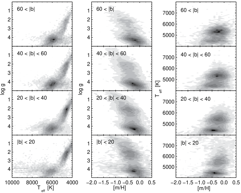
Following Paper II, in Fig. 18 we plot the location of all spectra on the temperature-gravity-metallicity wedge for different slices in Galactic latitude. The main-sequence and giant-star groups (particularly the red-clump branch) are clearly visible, with their relative frequency and metallicity distribution varying with latitude. For the hotter stars (${T_{\rm eff}}>9\,000\,$K) there is significant discretization in $\log g$. This is caused by the combination of a degeneracy in metallicity for these Paschen-line dominated spectra and a smaller range in possible $\log g$, which leads to the penalization algorithm having a tendency to converge on the same solution. Figure 19 plots histograms of the parameters for different latitudes. The fraction of main-sequence stars increases with the distance from the Galactic plane (see Paper 2 for a discussion). The metallicity distribution function becomes more metal poor for the higher-latitude fields as well. Also the shift of the temperature distribution towards higher temperature turn-off stars with decreasing Galactic latitude is clearly visible.

Figure 18: The temperature-gravity-metallicity plane for different wedges in Galactic latitude.

Figure 19: Temperature, gravity, and metallicity histograms for spectra with published stellar parameters. Histograms for individual Galactic latitude bands are plotted separately with the key given in the top panel. Spectra with $|b|\leq 20^{\circ}$ include calibration fields.

Table 10: Number and fraction of RAVE database entries with a counterpart in the photometric catalogs

Catalog name	Number of	% of entries	% with quality flag
	entries	with counterpart	A	B	C	D
Catalog A
2MASS	$57\,184$	$99.9\%$	$99.9\%$	$0.0\%$	$0.0\%$	$0.1\%$
DENIS	$43\,178$	$75.4\%$	$73.4\%$	$24.2\%$	$2.3\%$	$0.2\%$
USNO-B	$55\,686$	$97.2\%$	$99.3\%$	$0.5\%$	$0.0\%$	$0.1\%$
Catalog B
2MASS	$25\,699$	$99.6\%$	$99.4\%$	$0.0\%$	$0.0\%$	$0.6\%$
DENIS	$19\,433$	$75.3\%$	$74.5\%$	$22.6\%$	$2.2\%$	$0.7\%$
USNO-B	$25\,094$	$97.3\%$	$98.8\%$	$0.8\%$	$0.0\%$	$0.4\%$

Table 11: Summary of proper-motion sources and their average and 90% errors

SPM	Catalog	Number of	Fraction	Average	90%
Flag	Name	Entries	of entries	PM error	PM error
				[mas yr-1 ]	[mas yr-1 ]
	Catalog A
0	No proper motion	$595$	$1.0\%$
1	Tycho-2	$3\,517$	$6.1\%$	$3.2$	$4.3$
2	SSS	$1\,427$	$2.5\%$	$24.2$	$30.1$
3	PPMX	$24\,554$	$42.9\%$	$3.5$	$4.7$
4	2MASS + GSC 1.2	$30$	$0.0\%$	$18.8$	$27.3$
5	UCAC2	$24\,498$	$42.8\%$	$4.8$	$8.5$
6	USNO-B	$2\,651$	$4.6\%$	$5.7$	$8.6$
1-5	All with proper motion	$56\,677$	$99.0\%$	$4.7$	$7.4$
	Catalog B
0	No proper motion	$341$	$1.3\%$
1	Tycho-2	$300$	$1.2\%$	$3.4$	$4.7$
2	SSS	$2\,519$	$9.8\%$	$25.8$	$34.2$
3	PPMX	$6\,481$	$25.1\%$	$4.2$	$5.7$
4	2MASS + GSC 1.2	$32$	$0.1\%$	$22.0$	$26.4$
5	UCAC2	$13\,451$	$52.1\%$	$7.7$	$12.4$
6	USNO-B	$2\,676$	$10.4\%$	$5.3$	$8.5$
1-5	All with proper motion	$25459$	$98.7\%$	$8.3$	$13.6$

4.1 Photometry

As in the previous releases, DR3 includes cross-identifications with optical and near-IR catalogs (USNO-B: $B1$, $R1$, $B2$, $R2$; DENIS: $I$, $J$, $K$; 2MASS: $J$, $H$, $K$). The nearest-neighbor criterion was used for matching and we provide the distance to the nearest neighbor and a quality flag on the reliability of the match. Table 10 shows the completeness and flag statistics for the two catalogs, where we see that Catalog A’s coverage and quality are slightly better than those of Catalog B. This is because Catalog A is dominated by lower-magnitude objects while Catalog B contains mainly the higher-magnitude objects. For both, however, nearly all stars were successfully matched with the 2MASS and USNO-B catalogs. About 3/4 of the stars lie in the sky area covered by the DENIS catalog.

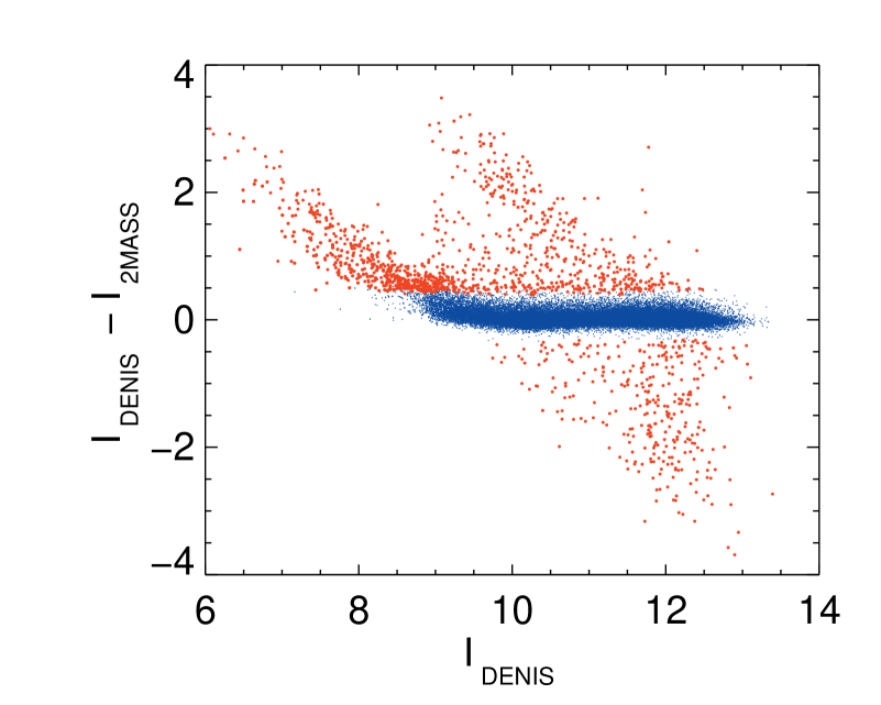
Our wavelength range is best represented by the $I$ filter. As discussed in detail in Paper II, there are some problems with a fraction of the DENIS $I$ magnitudes, particular for $I_{\mathrm{DENIS}}<10$, due to saturation effects. Following the methodology of DR2, we compare the DENIS magnitudes against an approximate one calculated from 2MASS J and K (see Equation 24 in Paper 2). Fig. 20 compares the DENIS and the “jury-rigged” 2MASS $I-$magnitudes for all stars in the current data release. We see that the two magnitudes agree for the majority of objects, but a significant fraction have large errors: $10\%$ have $|(I_{\mathrm{DENIS}}-I_{\mathrm{2MASS}})|>0.2$, with differences of up to 4 magnitudes. It was proposed in Paper II that $I_{\mathrm{DENIS}}$ magnitudes should be avoided when the condition

$$-0.2<(I_{\mathrm{DENIS}}-J_{\mathrm{2MASS}})-(J_{\mathrm{2MASS}}-K_{\mathrm{2MASS}})<0.6\,,$$ (3)

is not met. In Figure 20 we differentiate between the stars that do and do not satisfy this condition, where we see how it selects out the problematic $I_{\mathrm{DENIS}}$ magnitudes.

Figure 20: Difference between DENIS and jury-rigged 2MASS $I$ magnitudes as a function of $I_{\mathrm{DENIS}}$. The blue points are one satisfying equation 3, while the larger red points are ones that do not.

4.2 Proper motions

As in DR2, the proper motions are sourced from the PPMX, Tycho-2, SSS and UCAC2 catalogs. As described in Paper II, the most accurate available proper motion is chosen for each object. Table 11 summarizes for both Catalogs A and B the proper-motion sources and the average and $90^{\mathrm{th}}$ percentile errors. The quality of the proper motions is slightly worse for Catalog B, because the fainter objects in this catalog include a higher proportion of the more distant objects in the survey.

5 Conclusions

This third data release of the RAVE survey reports $83\,072$ radial-velocity measurements for $77\,461$ stars, covering more than $11\,500$ square degrees in the southern hemisphere. The sample is randomly selected in the magnitude interval $9\leq I\leq 12$. This release also provides stellar atmospheric parameters for $41\,672$ spectra representing $39\,833$ individual stars.

Since DR2, we modified the RAVE processing pipeline to account better for defects in the observed spectra due to bad pixels, fringing, or locally inaccurate continuum normalization. The main driver of the modification was to improve on the known limitation of our estimates of stellar atmospheric parameters. Also, the algorithm to correct for the zero-point offset has been revised, enabling a better control of our radial-velocity accuracy.

The accuracy for the radial velocities is marginally improved with the new pipeline, the distribution of internal errors in the radial velocities has mode $0.8\,\rm{km\,s}^{-1}$ and median $1.2\,\rm{km\,s}^{-1}$, and 95% of the sample having an internal error better than $5\,\rm{km\,s}^{-1}$, which is the primary objective of RAVE. Comparing our radial velocities to independent estimates based on 373 measurements from five data sources we find no evidence for a bias in our radial velocities, our mean radial velocity error being $\sim 2\,\rm{km\,s}^{-1}$.

A significant effort has been spent in improving the quality and validation of our stellar atmospheric parameters with respect to the external errors and biases. The internal errors due to the method and the sampling of synthetic spectra grid remain unchanged and are presented in Paper II. The new calibration sample consists of 362 stars from four different sources (either custom observations or literature) and cover the full HR diagram. Comparing our measured parameters to these reference measurements, we find a good agreement for ${T_{\rm eff}}$ and $\log g$ with a mean offset and dispersion of (-63, 250) K for ${T_{\rm eff}}$ and (-0.1, 0.43) dex for $\log g$, which are consistent with DR2. The $\mathrm{[m/H]}$ distribution is improved but the true metallicity $\mathrm{[M/H]}$ remains a combination of $\mathrm{[m/H]}$, $\mathrm{[\alpha/Fe]}$, and ${T_{\rm eff}}$. Taking $\log g$ or S/N  into the calibration of [M/H] only marginally improves the situation and the simplest calibration relation is preferred.

This data release is the last one based on the pilot-survey input catalog. Further releases will be based on an input catalog built upon DENIS-I magnitudes. This catalog, supplemented by the catalog of distances, make this release an unprecedented tool to study the Milky Way.

Appendix A

Table 12 describes the contents of individual columns of the Third Data Release catalog. The catalog is accessible online at www.rave-survey.org and via the Strasbourg astronomical Data Center (CDS) services.

Table 12: Catalog description

Column	Character	Format	Units	Symbol	Description
number	range
1	1- 16	A16	—	Name	Target designation
2	18- 34	A16	—	RAVEID	RAVE target designation
3	36- 48	F12.8	deg	RAdeg	Right ascension (J2000.0)
4	50- 62	F12.8	deg	DEdeg	Declination (J2000.0)
5	64- 73	F9.5	deg	GLON	Galactic longitude
6	75- 84	F9.5	deg	GLAT	Galactic latitude
7	86- 93	F7.1	$\!\,\rm{km\,s}^{-1}$	HRV	Heliocentric radial velocity
8	95-101	F6.1	$\!\,\rm{km\,s}^{-1}$	eHRV	HRV error
9	103-109	F6.1	mas yr-1	pmRA	proper motion RA
10	111-117	F6.1	mas yr-1	epmRA	error proper motion RA
11	119-125	F6.1	mas yr-1	pmDE	proper motion DE
12	127-133	F6.1	mas yr-1	epmDE	error proper motion DE
13	135-136	I1	—	Spm	source of proper motion (1)
14	138-143	F5.2	mag	Imag	Input catalog I magnitude
15	145-153	A8	—	Obsdate	Date of observation yyyymmdd
16	155-165	A10	—	FieldName	Name of RAVE field
17	167-168	I1	—	PlateNumber	Plate number used
18	170-173	I3	—	FiberNumber	Fiber number [1,150]
19	175-180	I5	K	Teff	Effective Temperature
20	182-186	F4.2	dex	logg	Gravity
21	188-193	F5.2	dex	Met	[m/H]
22	195-199	F4.2	dex	alpha	[Alpha/Fe]
23	201-209	F8.1	—	CHISQ	chi square
24	211-216	F5.1	—	S2N	DR2 signal to noise S2N
25	218-223	F5.1	—	STN	Pre-flux calibration signal to noise STN
26	225-230	F5.1	—	CorrelationCoeff	Tonry-Davis $R$ correlation coefficient
27	232-236	F4.2	—	PeakHeight	Height of correlation peak
28	238-244	F6.1	$\!\,\rm{km\,s}^{-1}$	PeakWidth	Width of correlation peak
29	246-252	F6.1	$\!\,\rm{km\,s}^{-1}$	CorrectionRV	Zero point correction applied
30	254-260	F6.1	$\!\,\rm{km\,s}^{-1}$	SkyRV	Measured HRV of sky
31	262-268	F6.1	$\!\,\rm{km\,s}^{-1}$	SkyeRV	error HRV of sky
32	270-275	F5.1	—	SkyCorrelation	Sky Tonry-Davis correl. coefficient
33	277-282	F5.1	—	SNRatio	Spectra signal to noise ratio
34	284-290	F6.3	mag	BT	Tycho-2 BT magnitude
35	292-298	F6.3	mag	eBT	error BT
36	300-306	F6.3	mag	VT	Tycho-2 VT magnitude
37	308-314	F6.3	mag	eVT	error VT
38	316-328	A12	—	USNOID	USNO-B designation
39	330-336	F6.3	mas	DisUSNO	Distance to USNO-B source
40	338-343	F5.2	mag	B1	USNO-B B1 magnitude
41	345-350	F5.2	mag	R1	USNO-B R1 magnitude
42	352-357	F5.2	mag	B2	USNO-B B2 magnitude
43	359-364	F5.2	mag	R2	USNO-B R2 magnitude
44	366-371	F5.2	mag	IUSNO	USNO-B I magnitude
45	373-374	A1	—	XidQualityUSNO	Cross-identification flag (2)
46	376-392	A16	—	DENISID	DENIS designation
47	394-400	F6.3	mas	DisDENIS	Distance to DENIS source
48	402-408	F6.3	mag	IDENIS	DENIS I magnitude
49	410-414	F4.2	mag	eIDENIS	error DENIS I magnitude
50	416-422	F6.3	mag	JDENIS	DENIS J magnitude
51	424-428	F4.2	mag	eJDENIS	error DENIS J magnitude
52	430-436	F6.3	mag	KDENIS	DENIS K magnitude
53	438-442	F4.2	mag	eKDENIS	error DENIS K magnitude
54	444-445	A1	—	XidQualityDENIS	Cross-identification flag (2)
55	447-463	A16	—	TWOMASSID	2MASS designation
56	465-471	F6.3	mas	Dis2MASS	Distance to 2MASS source
57	473-479	F6.3	mag	J2MASS	2MASS J magnitude
58	481-485	F4.2	mag	eJ2MASS	error 2MASS J magnitude
59	487-493	F6.3	mag	H2MASS	2MASS H magnitude
60	495-499	F4.2	mag	eH2MASS	error 2MASS H magnitude
61	501-507	F6.3	mag	K2MASS	2MASS K magnitude
62	509-513	F4.2	mag	eK2MASS	error 2MASS K magnitude
63	515-518	A3	—	TWOMASSphotFLAG	2MASS photometric flag
64	520-521	A1	—	XidQuality2MASS	Cross-identification flag (2)
65	523-526	A3	—	ZeroPointFLAG	Zero point correction flag (3)
66	528-536	A8	—	SpectraFLAG	Spectra quality flag (4)
67	538-542	F4.2	—	MaskFLAG	MASK flag (5)

Note. — (1): Flag value between 0 and 4: 0- no proper motion, 1- Tycho-2 proper motion, 2- Supercosmos Sky Survey proper motion, 3- PPMX proper motion, 4- GSC1.2 x 2MASS proper motion, 5- UCAC-2 proper motions.

(2): Flag value is A,B,C,D or X: A- good association, B- 2 solutions within 1 arcsec, C- more than two solutions within 1 arcsec, D- nearest neighbor more than 2 arcsec away, X- no possible counterpart found.

(3): Flag value of the form FGSH, F being for the entire plate, G for the 50 fibers group to which the fiber belongs. S flags the zero point correction used: C for cubic and S for a constant shift.If H is set to * the fiber is close to a 15 fiber gap. For F and G the values can be A, B, C, D or E: A- dispersion around correction lower than $1\,\rm{km\,s}^{-1}$, B- dispersion between 1 and $2\,\rm{km\,s}^{-1}$, C- dispersion between 2 and $3\,\rm{km\,s}^{-1}$, D- dispersion larger than $3\,\rm{km\,s}^{-1}$, E- less than 15 fibers available for the fit.

(4): Flag identifying possible problem in the spectra (values can be combined): a- asymmetric Ca lines, c- cosmic ray pollution, e- emission line spectra, n- noise dominated spectra, l- no lines visible, w- weak lines, g- strong ghost, t- bad template fit, s- strong residual sky emission, cc- bad continuum, r- red part of the spectra shows problem, b- blue part of the spectra shows problem, p- possible binary/doubled lined, x- peculiar object.

(5): Flag identifying the fraction of the spectrum unaffected by continuum problems from the MASK program. Spectrum with MaskFLAG lower than 0.70 must be used with caution.

References

- Anders & Grevesse (1989) Anders, E., & Grevesse, N., 1989, Geochimi. Cosmochim. Acta, 53, 197
- Breddels et al. (2010) Breddels, M. A., et al., 2010, A&A, 511,90
- Burnett & Binney (2010) Burnett, B. & Binney, J., 2010,MNRAS, 407, 339
- Burnett et al. (2011) Burnett, B., et al., 2010, A&A, in prep.
- Coşkunoǧlu et al. (2011) Coşkunoǧlu, B., et al., 2011, MNRAS, 412, 1237
- Eisenstein et al. (2011) Eisenstein, D., et al., 2011, AJ, submitted (arXiv:1101.1529)
- Famaey et al. (2005) Famaey, B., et al., 2005, A&A, 430, 165
- Fellhauer et al. (2006) Fellhauer, M., et al., 2006, ApJ, 651, 167
- Fulbright (2000) Fulbright, J.P., 2000, AJ, 120, 1841
- Fulbright et al. (2006) Fulbright, J.P., McWilliam, A., Rich, R.M., 2006, ApJ, 636, 821
- Fulbright et al. (2007) Fulbright, J.P., McWilliam, A., Rich, R.M., 2007, ApJ, 661, 1152
- Fulbright et al. (2010) Fulbright, J.P., et al., 2010, ApJL, 724, 104
- Kiss et al. (2011) Kiss, L.L., et al., 2011, MNRAS, 411, 117
- Klement et al. (2008) Klement, R., et al., 2008, ApJ, 685, 261
- Klement et al. (2011) Klement, R.J., Bailer-Jones, C.A.L., Fuchs, B., Rix, H.W., Smith, K.W., 2011, ApJ, 726, 103
- Matijevič et al. (2010) Matijevič, G., et al., 2010, AJ, 140, 184
- Matijevič et al. (2011) Matijevič, G., et al., 2011, AJ, submitted
- Munari et al. (2005) Munari, U., et al., 2005, A&A, 442, 1127
- Munari et al. (2008) Munari, U., et al., 2008, A&A, 488, 969
- Munari et al. (2009) Munari, U., et al., 2009, A&A, 503, 511
- Nordström et al. (2004) Nordström, B., et al., 2004, A&A,418,989
- Perryman et al. (1997) Perryman, M.A.C., et al., 1997, ESASP, 1200
- Ruchti et al. (2010) Ruchti, G.R., et al., 2010, ApJ, 721L, 92
- SDSS-III collaboration (2011) SDSS-III collaboration, 2011, ApJS, in press (arXiv:1101.1559)
- Seabroke et al. (2008) Seabroke, G., et al., 2008, MNRAS, 384, 11
- Soubiran & Girard (2005) Soubiran, C., & Girard, P., 2005, A&A, 438, 139
- Siebert et al. (2008) Siebert, A., et al., 2008, MNRAS, 391, 793
- Siebert et al. (2011) Siebert, A., et al., 2011, MNRAS, 412, 2026
- Smith et al. (2007) Smith, M. C., et al., 2007, MNRAS, 379, 755
- Steinmetz et al. (2006) Steinmetz, M., et al., 2006, AJ, 132, 1645 (Paper I)
- Veltz et al. (2008) Veltz, L., et al., 2008, A&A, 480,753
- Williams et al. (2011) Williams, M.E.K., et al., 2011, ApJ, 728, 102
- Wilson et al. (2011) Wilson, M.L., et al., 2011, MNRAS, in press (arXiv:1009.2052)
- Yanny et al. (2009) Yanny, B., et al., 2009, AJ,137,4377
- Zwitter et al. (2008) Zwitter, T., et al., 2008, AJ, 136, 421 (Paper II)
- Zwitter et al. (2010) Zwitter, T. et al., 2010, A&A, 522A, 54