Robust -Bit Compressive Sensing via
Binary Stable Embeddings
of Sparse Vectors111L. J. is funded by the Belgian Science
Policy “Return Grant”, BELSPO, IAP-VI BCRYPT, and by the Belgian F.R.S-FNRS.
J. L. and R. B. were supported by the
grants NSF CCF-0431150, CCF-0728867, CCF-0926127, CNS-0435425, and
CNS-0520280, DARPA/ONR N66001-08-1-2065, N66001-11-1-4090, ONR N00014-07-1-0936,
N00014-08-1-1067, N00014-08-1-1112, and N00014-08-1-1066, AFOSR
FA9550-07-1-0301 and FA9550-09-1-0432, ARO MURI W911NF-07-1-0185
and W911NF-09-1-0383, and the Texas Instruments Leadership
University Program. P.B. is funded by Mitsubishi Electric Research
Laboratories.
Abstract
The Compressive Sensing (CS) framework aims to ease the burden on analog-to-digital converters (ADCs) by reducing the sampling rate required to acquire and stably recover sparse signals. Practical ADCs not only sample but also quantize each measurement to a finite number of bits; moreover, there is an inverse relationship between the achievable sampling rate and the bit-depth. In this paper, we investigate an alternative CS approach that shifts the emphasis from the sampling rate to the number of bits per measurement. In particular, we explore the extreme case of 1-bit CS measurements, which capture just their sign. Our results come in two flavors. First, we consider ideal reconstruction from noiseless -bit measurements and provide a lower bound on the best achievable reconstruction error. We also demonstrate that i.i.d. random Gaussian matrices provide measurement mappings that, with overwhelming probability, achieve nearly optimal error decay. Next, we consider reconstruction robustness to measurement errors and noise and introduce the Binary -Stable Embedding (BSE) property, which characterizes the robustness of the measurement process to sign changes. We show that the same class of matrices that provide almost optimal noiseless performance also enable such a robust mapping. On the practical side, we introduce the Binary Iterative Hard Thresholding (BIHT) algorithm for signal reconstruction from 1-bit measurements that offers state-of-the-art performance.
1 Introduction
Recent advances in signal acquisition theory have led to significant interest in alternative sampling methods. Specifically, conventional sampling systems rely on the Shannon sampling theorem that states that signals must be sampled uniformly at the Nyquist rate, i.e., a rate twice their bandwidth. However, the compressive sensing (CS) framework describes how to reconstruct a signal from the linear measurements
| (1) |
where with is an underdetermined measurement system [1, 2]. It is possible to design a physical sampling system such that where is a vector of Nyquist-rate samples of a bandlimited signal , . In this case, (1) translates to low, sub-Nyquist sampling rates, providing the framework’s axial significance: CS enables the acquisition and accurate reconstruction of signals that were previously out of reach, limited by hardware sampling rates [3] or number of sensors [4].
Although inversion of (1) seems ill-posed, it has been demonstrated that -sparse signals, i.e., where , can be reconstructed exactly [1, 2]. To do this, we could naïvely solve for the sparsest signal that satisfies (1),
| (RCS) |
however, this non-convex program exhibits combinatorial complexity in the size of the problem [5]. Instead, we solve Basis Pursuit (BP) by relaxing the objective in (RCS) to the -norm; the result is a convex, polynomial-time algorithm [6]. A key realization is that, under certain conditions on , the BP solution will be equivalent to that of (RCS) [1]. This basic reconstruction framework has been expanded to include numerous fast algorithms as well as provably robust algorithms for reconstruction from noisy measurements [7, 8, 9, 10, 11]. Reconstruction can also be performed with iterative and greedy methods [12, 13, 14].
Reconstruction guarantees for BP and other algorithms are often demonstrated for that are endowed with the restricted isometry property (RIP), the sufficient condition that the norm of the measurements is close to the norm of the signal for all sparse [7].222The RIP is in fact not needed to demonstrate exact reconstruction guarantees in noiseless settings, however it proves quite useful for establishing robust reconstruction guarantees in noise. This can be expressed, in general terms, as a -stable embedding. Let and . We say the mapping is a -stable embedding of if
| (2) |
for all and . The RIP requires that (2) hold for all ; that is, it is a stable embedding of sparse vectors. A key result in the CS literature is that, if the coefficients of are randomly drawn from a sub-Gaussian distribution, then will satisfy the RIP with high probability as long as , for some constant [16, 17]. Several hardware inspired designs with only a few randomized components have also been shown to satisfy this property [18, 3, 19, 20].
In practice, CS measurements must be quantized, i.e., each measurement is mapped from a real value (over a potentially infinite range) to a discrete value over some finite range. For example, in uniform quantization, a measurement is mapped to one of distinct values, where denotes the number of bits per measurement. Quantization is an irreversible process that introduces error in the measurements. One way to account for quantization error is to treat it as bounded noise and employ robust reconstruction algorithms. Alternatively, we might try to reduce the error by choosing the most efficient quantizer for the distribution of the measurements. Several reconstruction techniques that specifically address CS quantization have also been proposed [21, 22, 23, 24, 25, 26].
While quantization error is a minor inconvenience, fine quantization invokes a more burdensome, yet often overlooked source of adversity: in hardware systems, it is the primary bottleneck limiting sample rates [27, 28]. In other words, the analog-to-digital converter (ADC) is beholden to the quantizer. First, quantization significantly limits the maximum speed of the ADC, forcing an exponential decrease in sampling rate as the number of bits is increased linearly [28]. Second, the quantizer is the primary power consumer in an ADC. Thus, more bits per measurement directly translates to slower sampling rates and increased ADC costs. Third, fine quantization is more susceptible to non-linear distortion in the ADC electronics, requiring explicit treatment in the reconstruction [29]. As we have seen, the CS framework provides one mechanism to alleviate the quantization bottleneck by reducing the ADC sampling rate. Is it possible to extend the CS framework to mitigate this problem directly in the quantization domain by reducing the number of bits per measurement (bit-depth) instead?
In this paper we concretely answer this question in the affirmative. We consider an extreme quantization; just one bit per CS measurement, representing its sign. The quantizer is thus reduced to a simple comparator that tests for values above or below zero, enabling extremely simple, efficient, and fast quantization. A -bit quantizer is also more robust to a number of commonly encountered non-linear distortions in the input electronics, as long as they preserve the signs of the measurements.
It is not obvious that the signs of the CS measurements retain enough information for signal reconstruction; for example, it is immediately clear that the scale (absolute amplitude) of the signal is lost. Nonetheless, there is strong empirical evidence that signal reconstruction is possible [30, 31, 32, 29]. In this paper we develop strong theoretical reconstruction and robustness guarantees, in the same spirit as classical guarantees provided in CS by the RIP.
We briefly describe the -bit CS framework proposed in [30]. Measurements of a signal are computed via
| (3) |
where the sign operator is applied component wise on , where equals if and otherwise, for any . Thus, the measurement operator is a mapping from to the Boolean cube333Generally, the -dimensional Boolean cube is defined as . Without loss of generality, we use instead. . At best, we hope to recover signals where is the unit hyper-sphere of dimension . We restrict our attention to sparse signals on the unit sphere since, as previously mentioned, the scale of the signal has been lost during the quantization process. To reconstruct, we enforce consistency on the signs of the estimate’s measurements, i.e., that . Specifically, we define a general non-linear reconstruction decoder such that, for , the solution is
-
(i)
sparse, i.e., satisfies ,
-
(ii)
consistent, i.e., satisfies .
With (RCS) from CS as a guide, one candidate program for reconstruction that respects these two conditions is
| (R1BCS) |
Although the parameter is not explicit in (R1BCS), the solution will be -sparse with because is a feasible point of the constraints.
Since (R1BCS) is computationally intractable, [30] proposes a relaxation that replaces the objective with the -norm and enforces consistency via a linear convex constraint. However, the resulting program remains non-convex due to the unit-sphere requirement. Be that as it may, several optimization algorithms have been developed for the relaxation, as well as a greedy algorithm inspired by the same ideas [30, 31, 32]. While previous empirical results from these algorithms provide motivation for the validity of this -bit framework, there have been few analytical guarantees to date.
The primary contribution of this paper is a rigorous analysis of the -bit CS framework. Specifically, we examine how the reconstruction error behaves as we increase the number of measurement bits given the signal dimension and sparsity . We provide two flavors of results. First, we determine a lower bound on reconstruction performance from all possible mappings with the reconstruction decoder , i.e., the best achievable performance of this -bit CS framework. We further demonstrate that if the elements of are drawn randomly from Gaussian distribution or its rows are drawn uniformly from the unit sphere, then the worst-case reconstruction error using will decay at a rate almost optimal with the number of measurements, up to a log factor in the oversampling rate and the signal dimension . Second, we provide conditions on that enable us to characterize the reconstruction performance even when some of the measurement signs have changed (e.g., due to noise in the measurements). In other words, we derive the conditions under which robust reconstruction from -bit measurements can be achieved. We do so by demonstrating that is a stable embedding of sparse signals, similar to the RIP. We apply these stable embedding results to the cases where we have noisy measurements and signals that are not strictly sparse. Our guarantees demonstrate that the -bit CS framework is on sound footing and provide a first step toward analysis of the relaxed -bit techniques used in practice.
To develop robust reconstruction guarantees, we propose a new tool, the binary -stable embedding (BSE), to characterize -bit CS systems. The BSE implies that the normalized angle between any sparse vectors in is close to the normalized Hamming distance between their -bit measurements. We demonstrate that the same class of random as above exhibit this property when (where is some constant). Thus remarkably, there exist such that the BSE holds when both the number of measurements is smaller than the dimension of the signal and the measurement bit-depth is at minimum.
As a complement to our theoretical analysis, we introduce a new -bit CS reconstruction algorithm, Binary Iterative Hard Thresholding (BIHT). Via simulations, we demonstrate that BIHT yields a significant improvement in both reconstruction error as well as consistency, as compared with previous algorithms. To gain intuition about the behavior of BIHT, we explore the way that this algorithm enforces consistency and compare and contrast it with previous approaches. Perhaps more important than the algorithm itself is the discovery that the BIHT consistency formulation provides a significantly better feasible solution in noiseless settings, as compared with previous algorithms. Finally, we provide a brief explanation regarding why this new formulation achieves better solutions, and its connection with results in the machine learning literature.
Since the first appearance of this work, Plan and Vershynin have developed additional theoretical results and bounds on the performance of 1-bit CS, as well as two convex algorithms with theoretical guarantees [33, 34, 35]. The results in [33, 34] generalize the BSE guarantees for more general classes of signals, including compressible signals in addition to simply sparse ones. However, the guarantees provided in that work exhibit worse decay rates in the error performance and the tightness of the BSE property. Furthermore, the results of [34, 35] are intimately tied to reconstruction algorithms, in contrast to our analysis. We point out similarities and differences with our results when appropriate in the subsequent development.
In addition to benchmarking the performance of BIHT, our simulations demonstrate that many of the theoretical predictions that arise from our analysis (such as the error rate as a function of the number of measurements or the error rate as a function of measurement Hamming distance), are actually exhibited in practice. This suggests that our theoretical analysis is accurately explaining the true behavior of the framework.
The remainder of this paper is organized as follows. In Section 2, we develop performance results for -bit CS in the noiseless setting. Specifically we develop a lower bound on reconstruction performance as well as provide the guarantee that Gaussian matrices enable this performance. In Section 3 we introduce the notion of a BSE for the mapping and demonstrate that Gaussian matrices facilitate this property. We also expand reconstruction guarantees for measurements with Gaussian noise (prior to quantization) and non-sparse signals. To make use of these results in practice, in Section 4 we present the BIHT algorithm for practical -bit reconstruction. In Section 5 we provide simulations of BIHT to verify our claims. In Section 6 we conclude with a discussion about implications and future extensions. To facilitate the flow of the paper and clear descriptions of the results, most of our proofs are provided in the appendices.
2 Noiseless Reconstruction Performance
2.1 Reconstruction performance lower bounds
In this section, we seek to provide guarantees on the reconstruction error from -bit CS measurements. Before analyzing this performance from a specific mapping with the consistent sparse reconstruction decoder , it is instructive to determine the best achievable performance from measurements acquired using any mapping. Thus, in this section we seek a lower bound on the reconstruction error.
We develop the lower bound on the reconstruction error based on how well the quantizer exploits the available measurement bits. A distinction we make in this section is that of measurement bits, which is the number of bits acquired by the measurement system, versus information bits, which represent the true amount of information carried in the measurement bits. Our analysis follows similar ideas to that in [36, 37], adapted to sign measurements.
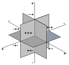
We first examine how 1-bit quantization operates on the measurements. Specifically, we consider the orthants of the measurement space. An orthant in is the set of vectors such that all the vector’s coefficients have the same sign pattern
| (4) |
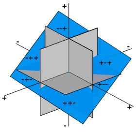
where . Notice that and if . Therefore, any -dimensional space is partitioned to orthants. Figure 1(a) shows the 8 orthants of as an example. Since 1-bit quantization only preserves the signs of the measurements, it encodes in which measurement space orthant the measurements lie. Thus, each available quantization point corresponds to an orthant in the measurement space. Any unquantized measurement vector that lies in an orthant of the measurement space will quantize to the corresponding quantization point of that orthant and cannot be distinguished from any other measurement vector in the same orthant. To obtain a lower bound on the reconstruction error, we begin by bounding the number of quantization points (or equivalently the number of orthants) that are used to encode the signal.
While there are generally orthants in the measurement space, the space formed by measuring all sparse signals occupies a small subset of the available orthants. We determine the number of available orthants that can be intersected by the measurements in the following lemma:
Lemma 1.
Let belong to a union of subspaces of dimension , and let -bit measurements be acquired via the mapping as defined in (3). Then the measurements can effectively use at most quantization points, i.e., carry at most information bits.
Proof.
A -dimensional subspace in an -dimensional space cannot lie in all the available octants. For example, as shown in Fig. 1(b), a 2-dimensional subspace of a 3-dimensional space can intersect at most 6 of the available octants. In Appendix A, we demonstrate that one arbitrary -dimensional subspace in an -dimensional space intersects at most orthants of the available. Since is a linear operator, any -dimensional subspace in the signal space is mapped through to a subspace that is also at most -dimensional and therefore follows the same bound. Thus, if the signal of interest belongs in a union of such -dimensional subspaces, then , and it follows that at most orthants are intersected. This means that at most effective quantization points can be used, i.e., at most information bits can be obtained.
Since -sparse signals in any basis belong to a union of at most subspaces in with , using Lemma 1 we can obtain the following corollary.444This corollary is easily adaptable to a redundant frame with .
Corollary 1.
Let be -sparse in a certain basis , i.e., . Then the measurements can effectively use at most 1-bit quantization points, i.e, carry at most information bits.
The set of signals of interest to be encoded is the set of unit-norm -sparse signals . Since unit-norm signals of a -dimensional subspace form a -dimensional unit sphere in that subspace, is a union of such unit spheres. The available quantization points partition into smaller sets, each of which contains all the signals that quantize to the same point.
To develop the lower bound on the reconstruction error we examine how can be optimally partitioned with respect to the worst-case error, given the number of quantization points used. The measurement and reconstruction process maps each signal in to a finite set of quantized signals . At best this map ensures that the worst case reconstruction error is minimized, i.e.,
| (5) |
where denotes the worst-case quantization error and each of the available quantization points. The optimal lower bound is achieved by designing to minimize (5) without considering whether the measurement and reconstruction process actually achieve this design. Thus, designing the set becomes a set covering problem. Appendix B precises this intuition and proves the following statement.
Theorem 1.
Thus, when is high compared to , the worst-case error cannot decay at a rate faster than as a function of the number measurements, no matter what reconstruction algorithm is used.
This result assumes noiseless acquisition and provides no guarantees of robustness and noise resiliency. This is in line with existing results on scalar quantization in oversampled representations and CS that state that the distortion due to scalar quantization of noiseless measurements cannot decrease faster than the inverse of the measurement rate [37, 38, 39, 40, 36].
To improve the rate vs. distortion trade-off, alternative quantization methods must be used, such as Sigma-Delta () quantization [41, 42, 43, 44, 45, 46, 47] or non-monotonic scalar quantization [48]. Specifically, approaches to CS can achieve error decay rate of , where is the order of the quantizer [47]. However, quantization requires feedback during the quantization process, which is not necessary in scalar quantization. Furthermore, the result in [47] only holds for multibit quantizers, not 1-bit ones. While efficient 1-bit quantization has been shown for classical sampling [42, 49], to the best of our knowledge, similar results are not currently known for 1-bit in CS applications. Alternatively, non-monotonic scalar quantization can achieve error decay exponential in the number of measurements , even in CS applications [48]. However, such a scheme requires a significantly more complex scalar quantizer and reconstruction approach [50].
Theorem 1 bounds the best possible performance of a consistent reconstruction over all possible mappings . However, not all mappings will behave as the lower bound suggests. In the next section we identify two classes of matrices such that the mapping admits an upper bound on the reconstruction error from a general decoder that decays almost optimally.
2.2 Achievable performance via random projections
In this section we describe a class of matrices such that the consistent sparse reconstruction decoder can indeed achieve error decay rates of optimal order, described by Theorem 1, with the number of measurements growing linearly in the sparsity and logarithmically in the dimension , as is required in conventional CS. We first focus our analysis on Gaussian matrices, i.e., such that each element is randomly drawn i.i.d. from the standard Gaussian distribution, . In the rest of the paper, we use the short notation to characterize such matrices, and we write to describe the equivalent random vectors in (e.g., the rows of ). For these matrices , we prove the following in Appendix C.
Theorem 2.
Let be matrix generated as , and let the mapping be defined as in (3). Fix and . If the number of measurements is
| (6) |
then for all we have that
| (7) |
or equivalently
with probability higher than .
Theorem 2 is a uniform reconstruction result, meaning that with high probability all vectors can be reconstructed as opposed to a non-uniform result where each vector could be reconstructed with high probability.
As derived in Appendix G, Theorem 2 demonstrates that if we use Gaussian matrices in the mapping , then, given a fixed probability level , the reconstruction decoder will recover signals with error order
which decays almost optimally compared to the lower bound given in Theorem 1 up to a log factor in . Whether the gap can be closed, with tighter lower or upper bounds is still an open question. Notice that the hidden proportionality factor in this last relation depends linearly on which is assumed fixed.
We should also note a few minor extensions of Theorem 2. We can multiply the rows of with a positive scalar without changing the signs of the measurements. By normalizing the rows of the Gaussian matrix we obtain another class of matrices, ones with rows drawn uniformly from the unit sphere in . It is thus straightforward to extend the Theorem to matrices with such rows as well. Furthermore, these projections are rotation invariant (often referred to as “universal” in CS systems), meaning that the theorem remains valid for sparse signals in any basis , i.e., for belonging to . This is true since for any orthonormal basis , when .
2.3 Related Work
A similar result to Theorem 2 has been recently shown for sign measurements of non-sparse signals in the context of quantization using frame permutations [51]. Specifically, it has been shown that reconstruction from sign measurements of signals can be achieved (almost surely) with an error rate decay arbitrarily close to . Our main contribution here is demonstrating that this result is true uniformly for all -sparse vectors in , given a sparse and consistent decoder. Our results, in addition to introducing the almost linear dependence on , also show that proving this error bound uniformly for all -sparse signals involves a logarithmic penalty in . This does not seem to be necessary from the lower bound in the previous section. We will see in Section 5 that for Gaussian matrices, the optimal error behavior is empirically exhibited on average. Finally, we note that for a constant , the number of measurements required to guarantee (7) is , nearly the same as order in conventional CS.
Furthermore, since the first appearance of our work, a bound on the achievable reconstruction error for compressible signals and for signals in arbitrary subsets of appeared in [33, 34]. Specifically for compressible signals, that works leads to error decay , which decreases more slowly (with ) than both our bound and the one provided in [51]. However, the results in [33, 34] are for more general classes of signals.
We can also view the binary measurements as a hash or a sketch of the signal. With this interpretation of the result we guarantee with high probability that no sparse vectors with Euclidean distance greater than will “hash” to the same binary measurements. In fact, similar results play a key role in locality sensitive hashing (LSH), a technique that aims to efficiently perform approximate nearest neighbors searches from quantized projections [52, 53, 54, 55]. Most LSH results examine the performance on point-clouds of a discrete number of signals instead of the infinite subspaces that we explore in this paper. Furthermore, the primary goal of the LSH is to preserve the structure of the nearest neighbors with high probability. Instead, in this paper we are concerned with the ability to reconstruct the signal from the hash, as well as the robustness of this reconstruction to measurement noise and signal model mismatch. To enable these properties, we require a property of the mapping that preserves the structure (geometry) of the entire signal set. Thus, in the next section we seek an embedding property of that preserves geometry for the set of sparse signals and thus ensures robust reconstruction.
3 Acquisition and Reconstruction Robustness
3.1 Binary -stable embeddings
In this section we establish an embedding property for the -bit CS mapping that ensures that the sparse signal geometry is preserved in the measurements, analogous to the RIP for real-valued measurements. This robustness property enables us to upper bound the reconstruction performance even when some measurement signs have been changed due to noise. Conventional CS achieves robustness via the -stable embeddings of sparse vectors (2) discussed in Section 1. This embedding is a restricted quasi-isometry between the metric spaces and , where the distance metrics and are the -norm in dimensions and , respectively, and the domain is restricted to sparse signals.555A function is called a quasi-isometry between metric spaces and if there exists and such that for , and such that for all [56]. Since for -stable embeddings, they are also called bi-Lipschitz mappings. We seek a similar definition for our embedding; however, now the signals and measurements lie in the different spaces and , respectively. Thus, we first consider appropriate distance metrics in these spaces.
The Hamming distance is the natural distance for counting the number of unequal bits between two measurement vectors. Specifically, for we define the normalized Hamming distance as
where is the XOR operation between such that equals 0 if and 1 otherwise. The distance is normalized such that . In the signal space we only consider unit-norm vectors, thus, a natural distance is the angle formed by any two of these vectors. Specifically, for , we consider
As with the Hamming distance, we normalize the true angle such that . Note that since both vectors have the same norm, the inner product can easily be mapped to the -distance using the polarization identity.
Using these distance metrics we define the binary stable embedding.
Definition 1 (Binary -Stable Embedding).
Let . A mapping is a binary -stable embedding (BSE) of order for sparse vectors if
for all with .
Our definition describes a specific quasi-isometry between the two metric spaces and , restricted to sparse vectors. While this mirrors the form of the -stable embedding for sparse vectors, one important difference is that the sensitivity term is additive, rather than multiplicative, and thus the BSE is not bi-Lipschitz. This is a necessary side-effect of the loss of information due to quantization.
Any BSE of order enables robustness guarantees on any reconstruction algorithm extracting a unit sparse signal estimate of . In this case, the angular error is immediately bounded by
Thus, if an algorithm returns a unit norm sparse solution with measurements that are not consistent (i.e., ), as is the case with several algorithms [30, 31, 32], then the worst-case angular reconstruction error is close to Hamming distance between the estimate’s measurements’ signs and the original measurements’ signs. Section 5 verifies this behavior with simulation results. Furthermore, in Section 3.3 we use the BSE property to guarantee that if measurements are corrupted by noise or if signals are not exactly sparse, then the reconstruction error is bounded.
Note that, in the best case, for a BSE , the angular error of any sparse and consistent decoder is bounded by since then . As we have seen earlier this is to be expected because, unlike conventional noiseless CS, quantization fundamentally introduces uncertainty and exact recovery cannot be guaranteed. This is an obvious consequence of the mapping of the infinite set to a discrete set of quantized values.
We next identify a class of matrices for which is a BSE.
3.2 Binary -stable embeddings via random projections
As is the case for conventional CS systems with RIP, designing a for -bit CS such that has the BSE property is possibly a computationally intractable task (and no such algorithm is yet known). Fortunately, an overwhelming number of “good” matrices do exist. Specifically we again focus our analysis on Gaussian matrices as in as in Section 2.2. As motivation that this choice of will indeed enable robustness, we begin with a classical concentration of measure result for binary measurements from a Gaussian matrix.
Lemma 2.
Let be a pair of arbitrary fixed vectors, draw according to , and let the mapping be defined as in (3). Fix . Then we have
| (8) |
where the probability is with respect to the generation of .
Proof.
This lemma is a simple consequence of Lemma 3.2 in [57] which shows that, for one measurement, . The result then follows by applying Hoeffding’s inequality to the binomial random variable with trials.
In words, Lemma 2 implies that the Hamming distance between two binary measurement vectors tends to the angle between the signals and as the number of measurements increases. In [57] this fact is used in the context of randomized rounding for max-cut problems; however, this property has also been used in similar contexts as ours with regards to preservation of inner products from binary measurements [58, 59].
The expression (8) indeed looks similar to the definition of the BSE, however, it only holds for a fixed pair of arbitrary (not necessarily sparse) signals, chosen prior to drawing . Our goal is to extend (8) to cover the entire set of sparse signals. Indeed, concentration results similar to Lemma 2, although expressed in terms of norms, have been used to demonstrate the RIP [16]. These techniques usually demonstrate that the cardinality of the space of all sparse signals is sufficiently small, such that the concentration result can be applied to demonstrate that distances are preserved with relatively few measurements.
Unfortunately, due to the non-linearity of we cannot immediately apply Lemma 2 using the same procedure as in [16]. To briefly summarize, [16] proceeds by covering the set of all -sparse signals with a finite set of points (with covering radius ). A concentration inequality is then applied to this set of points. Since any sparse signal lies in a -neighborhood of at least one such point, the concentration property can be extended from the finite set to by bounding the distance between the measurements of the points within the -neighborhood. Such an approach cannot be used to extend (8) to , because the severe discontinuity of our mapping does not permit us to characterize the measurements using and and obtain a bound on the distance between measurements of signals in a -neighborhood.
To resolve this issue, we extend Lemma 2 to include all points within Euclidean balls around the vectors and inside the (sub) sphere for some fixed support set of size . Define the -ball to be the ball of Euclidean distance around , and let .
Lemma 3.
Given of size , let be a matrix generated as , and let the mapping be defined as in (3). Fix and . For any , we have
The proof of this result is given in Appendix D. It should be noted that the proof does not depend on the radial behavior of the Gaussian pdf in . In other words, this result is easily generalizable to matrices whose rows are independent random vectors drawn from an isotropic pdf .
In words, if the width is sufficiently small, then the Hamming distance between the -bit measurements , of any points , within the balls , , respectively, will be close to the angle between the centers of the balls.
Lemma 3 is key for providing a similar argument to that in [16]. We now simply need to count the number of pairs of -sparse signals that are euclidean distance apart. The Lemma can then be invoked to demonstrate that the angles between all of these pairs will be approximately preserved by our mapping.666 We note that the covering argument in the proof of Theorem 2 also employs -balls in similar fashion but only considers the probability that , rather than the concentration inequality. Thus, with Lemma 3 under our belt, we demonstrate in Appendix E the following result.
Theorem 3.
Let be a matrix generated as and let the mapping be defined as in (3). Fix and . If the number of measurements is
| (9) |
then with probability exceeding , the mapping is a BSE of order for sparse vectors.
As with Lemma 3, the theorem extends easily to matrices with independent rows in drawn from an isotropic pdf in this space.
By choosing with , with high probability we ensure that the mapping is a BSE. Additionally, using (9) with a fixed and the development in Appendix G, we find that the error decreases as
Unfortunately, this decay rate is slower, roughly by a factor of , than the lower bound in Section 2.1. This error rate results from an application of the Chernoff-Hoeffding inequality in the proof of Theorem 3. An open question is whether it is possible to obtain a tighter bound (with optimal error rate) for this robustness property.
As with Theorem 2, Gaussian matrices provide a universal mapping, i.e., the result remains valid for sparse signals in a basis . Moreover, Theorem 3 can also be extended to rows of that are drawn uniformly on the sphere, since the rows of in Theorem 3 can be normalized without affecting the outcome of the proof. Note that normalizing the Gaussian rows of is as if they had been drawn from a uniform distribution of unit-norm signals.
We have now established a random construction providing robust BSEs with high probability: -bit quantized Gaussian projections. We now make use of this robustness by considering an example where the measurements are corrupted by Gaussian noise.
3.3 Noisy measurements and compressible signals
In practice, hardware systems may be inaccurate when taking measurements; this is often modeled by additive noise. The mapping is robust to noise in an unusual way. After quantization, the measurements can only take the values or . Thus, we can analyze the reconstruction performance from corrupted measurements by considering how many measurements flip their signs. For example, we analyze the specific case of Gaussian noise on the measurements prior to quantization, i.e.,
| (10) |
where has i.i.d. elements . In this case, we demonstrate, via the following lemma, a bound on the Hamming distance between the corrupted and ideal measurements with the BSE from Theorem 3 (see Appendix F).
Lemma 4.
If is the estimate from a sparse consistent reconstruction decoder from the measurements with and if satisfies (9), then it immediately follows from Lemma 4 and Theorem 3 that
| (11) |
with a probability higher than . Given alternative noise distributions, e.g., Poisson noise, a similar analysis can be carried out to determine the likely number of sign flips and thus provide a bound on the error due to noise.
Another practical consideration is that real signals are not always strictly -sparse. Indeed, it may be the case that signals are compressible; i.e., they can be closely approximated by a -sparse signal. In this case, we can reuse the non-uniform result of Lemma 2 to see that, given and for ,
In similar fashion to (11), if satisfies (9), this result and Theorem 3 imply that, given (not necessarily sparse) and for the angular reconstruction error of is such that , with probability higher than . Therefore, from the triangular inequality on , this provides the bound
with the same probability. Much like conventional CS results, the reconstruction error depends on the magnitude of the best -term approximation error of the signal, here expressed angularly by .
This reconstruction error bound is non-uniform with respect to the selection of . A uniform bound on the BSE for more general classes of signals is developed in [33, 34], albeit with a worse error decay— for compressible signals.
Thus far we have demonstrated a lower bound on the reconstruction error from -bit measurements (Theorem 2) and introduced a condition on the mapping that enables stable reconstruction in noiseless, noisy, and compressible settings (Definition 1). We have furthermore demonstrated that a large class of random matrices—specifically matrices with coefficients drawn from a Gaussian distribution and matrices with rows drawn uniformly from the unit sphere—provide good mappings (Theorem 3).
Using these results we can characterize the error performance of any algorithm that reconstructs a -sparse signal. If the reconstructed signal quantizes to the same quantization point as the original data, then the error is characterized by Theorem 2. If the algorithm terminates unable to reconstruct a signal consistent with the quantized data, then Theorem 3 describes how far the solution is from the original signal. Since (R1BCS) is a combinatorially complex problem, in the next section we describe a new greedy reconstruction algorithm that attempts to find a solution as consistent with the measurements as possible, while guaranteeing this solution is -sparse.
4 BIHT: A Simple First-Order Reconstruction Algorithm
4.1 Problem formulation and algorithm definition
We now introduce a simple algorithm for the reconstruction of sparse signals from -bit compressive measurements. Our algorithm, Binary Iterative Hard Thresholding (BIHT), is a simple modification of IHT, the real-valued algorithm from which is takes its name [14]. Demonstrating theoretical convergence guarantees for BIHT is a subject of future work (and thus not shown in this paper), however the algorithm is of significant value since it i) has a simple and intuitive formulation and ii) outperforms previous algorithms empirically, demonstrated in Section 5. We further note that the IHT algorithm has recently been extended to handle measurement non-linearities [60]; however, these results do not apply to quantized measurements since quantization does not satisfy the requirements in [60].
We briefly recall that the IHT algorithm consists of two steps that can be interpreted as follows. The first step can be thought of as a gradient descent to reduce the least squares objective . Thus, at iteration , IHT proceeds by setting . The second step imposes a sparse signal model by projecting onto the “ ball”, i.e., selecting the largest in magnitude elements. Thus, IHT for CS can be thought of as trying to solve the problem
| (12) |
The BIHT algorithm simply modifies the first step of IHT to instead minimize a consistency-enforcing objective. Specifically, given an initial estimate and -bit measurements , at iteration BIHT computes
| (13) | ||||
| (14) |
where is defined as in (3), is a scalar that controls gradient descent step-size, and the function computes the best -term approximation of by thresholding. Once the algorithm has terminated (either consistency is achieved or a maximum number of iterations have been reached), we then normalize the final estimate to project it onto the unit sphere. Section 4.2 discusses several variations of this algorithm, each with different properties.
The key to understanding BIHT lies in the formulation of the objective. The following Lemma shows that the term in (13) is in fact the negative subgradient of a convex objective . Let denote the negative function, i.e., with if and 0 else, and denote the Hadamard product, i.e., for two vectors and .
Lemma 5.
The quantity in (13) is a subgradient of the convex one-sided -norm
Thus, BIHT aims to decrease at each step (13).
Proof.
We first note that is convex. We can write with each convex function given by
where denotes a row of and . Moreover, if , then the gradient of is
while if , then the gradient is replaced by the subdifferential set
Thus, by summing over we conclude that .
Consequently, the BIHT algorithm can be thought of as trying to solve the problem:
Observe that since simply scales the elements of by the signs , minimizing the one-sided objective enforces a positivity requirement,
| (15) |
that, when satisfied, implies consistency.
Previously proposed -bit CS algorithms have used a one-sided -norm to impose consistency [30, 31, 32, 29]. Specifically, they have applied a constraint or objective that takes the form . Both the one-sided and functions imply a consistent solution when they evaluate to zero, and thus, both approaches are capable of enforcing consistency. However, the choice of the vs. penalty term makes a significant difference in performance depending on the noise conditions. We explore this difference in the experiments in Section 5.
4.2 BIHT shifts
Several modifications can be made to the BIHT algorithm that may improve certain performance aspects, such as consistency, reconstruction error, or convergence speed. While a comprehensive comparison is beyond the scope of this paper, we believe that such variations exhibit interesting and useful properties that should be mentioned.
Projection onto sphere at each iteration. We can enforce that every intermediate solution have unit norm. To do this, we modify the “impose signal model” step (14) by normalizing after choosing the best -term approximation, i.e., we replace the update of in (14) by , where . While this step is found in previous algorithms such as [30, 31, 32], empirical observations suggest that it not required for BIHT to converge to an appropriate solution.
If we choose to impose the projection, must be appropriately normalized or, equivalently, the step size of the gradient descent must be carefully chosen. Otherwise, the algorithm will not converge. Empirically, we have found that for a Gaussian matrix, an appropriate scaling is , where the controls the amplification of the estimate from in the gradient descent step (13) and the ensures that . Similar gradient step scaling requirements have been imposed in the conventional IHT algorithm and other sparse recovery algorithms as well (e.g., [9]).
Minimizing hinge loss. The one-sided -norm is related to the hinge-loss function in the machine learning literature, which is known for its robustness to outliers [61]. Binary classification algorithms seek to enforce the same consistency function as in (15) by minimizing a function , where sets negative elements to zero. When , the objective is both convex and has a non-trivial solution. Further connections and interpretations are discussed in Section 5. Thus, rather than minimizing the one-sided norm, we can instead minimize the hinge-loss. The hinge-loss can be interpreted as ensuring that the minimum value that an unquantized measurement can take is bounded away form zero, i.e., . This requirement is similar to the sphere constraint in that it avoids a trivial solution; however, will perform differently than the sphere constraint. In this case, in the gradient descent step (13), we instead compute
where scales the rows of by the signs of . Again, the step size must be chosen appropriately, this time as , where is a parameter that depends on .
General one-sided objectives. In general, any function , where is continuous and has a negative gradient for and is for , can be used to enforce consistency. To employ such functions, we simply compute the gradient of and apply it in (13). As an example, the previously mentioned one-sided -norm has been used to enforce consistency in several algorithms. We can use it in BIHT by computing
in (13). We compare and contrast the behavior of the one-sided and norms in Section 5.
As another example, in similar fashion to the Huber norm [15], we can combine the and functions in a piecewise fashion. One potentially useful objective is , where is defined as follows:
| (16) |
While similar, this is not exactly a one-sided Huber norm. In a one-sided Huber-norm, the square () term would be applied to values near zero and the magnitude () term would be applied to values significantly less than zero, the reverse of what we propose here.
This hybrid objective can provide different robustness properties or convergence rates than the previously mentioned objectives. Specifically, during each iteration it may allow us to take advantage of the shallow gradient of the one-sided cost for large numbers of measurement sign discrepancies and the steeper gradient of the one-sided cost when most measurements have the correct sign. This objective can be applied in BIHT as with the other objectives, by computing its gradient and plugging it into (13).
5 Experiments
In this section we explore the performance of the BIHT algorithm and compare it to the performance of previous -bit CS algorithms. To make the comparison as straightforward as possible, we reproduced the experiments of [32] with the BIHT algorithm.
The experimental setup is as follows. For each data point, we draw a length-, -sparse signal with the non-zero entries drawn uniformly at random on the unit sphere, and we draw a new matrix with each entry . We then compute the binary measurements according to (3). Reconstruction of is performed from with three algorithms: matching sign pursuit (MSP) [31], restricted-step shrinkage (RSS) [32], and BIHT (this paper); the algorithms will be depicted by dashed, dotted, and triangle lines, respectively. Each reconstruction in this setup is repeated for 1000 trials and with a fixed and unless otherwise noted. Furthermore, we perform the trials for within the range . Note that when , we are acquiring more measurements than the ambient dimension of the signal. While the regime is not interesting in conventional CS, it may be very practical in -bit systems that can acquire sign measurements at extremely high, super-Nyquist rates.
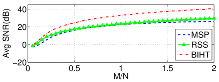
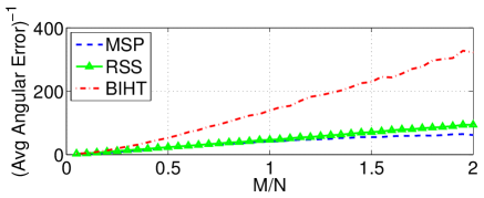
Average error. We begin by measuring the average reconstruction angular error over the trials. Figure 2 displays the results of this experiment in two different ways: (i) the signal-to-noise ratio (SNR)777In this paper we define the reconstruction SNR in decibels as . Note that this metric uses the standard euclidean error and not angular error. in Figure 2(a), to demonstrate that the performance of these techniques is practical (since the angular error is unintuitive to most observers), and (ii) the inverse of the angular error, i.e., in Figure 2(b), to compare with the performance predicted by Theorem 2.
We begin by comparing the performance of the algorithms. While we can observe that the angular error of each algorithm follows the same trend, BIHT obtains smaller error (or higher SNR) than the others, significantly so when is greater than . The discrepancy in performance could be due to difference in the algorithms themselves, or perhaps, differences in their formulations for enforcing consistency. This is explored later in this section.
We now consider the actual performance trend. We see from Figure 2(b) that, above each line appears fairly linear, albeit with a different slope, implying that with all other variables fixed, . This is on the order of the optimal performance as given by the bound given in Theorem 1 and predicted by Theorem 2 for Gaussian matrices.
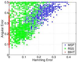
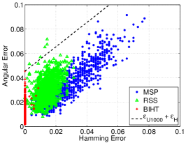
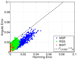
Consistency. We also expose the relationship between the Hamming distance between the measurements of the true and reconstructed signal and the angular error of the true and reconstructed signal. Figure 3 depicts the Hamming distance vs. angular error for three different values of . The particularly striking result is that BIHT returns significantly more consistent reconstructions than the two other algorithms. We observed this effect for ratio as small as (Figure 3(a)). This is clear from the fact that most of the red (plus) points lie on the y-axis while the majority of blue (dot) or green (triangle) points do not. We find that, even in significantly “under-sampled” regimes like , where the BSE is unlikely to hold, BIHT is likely to return a consistent solution (albeit with high variance of angular errors). We also find that in “over-sampled” regimes such as , the range of angular errors on the y-axis is small. Indeed, the range of angular errors shrinks as increases, implying an imperical tightening of the BSE upper and lower bounds.
We can infer an interesting performance trend from Figures 3(b) and (c), where the BSE property may hold. Since the RSS and MSP algorithms often do not return a consistent solution, we can visualize the relationship between angular error and hamming error. Specifically, on average the angular reconstruction error is a linear function of hamming error, , as similarly expressed by the reconstruction error bound provided by BSE. Furthermore, if we let be the largest angular error (with consistent measurements) over trials, then we can suggest an empirical upper bound for BIHT of . This upper bound is denoted by the dashed line in Figures 3(b) and (c).
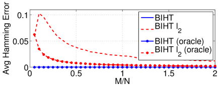
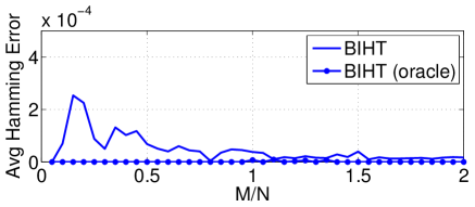
One-sided vs. one-sided objectives. As demonstrated in Figures 2 and 3, the BIHT algorithm achieves significantly improved performance over MSP and RSS in both angular error and Hamming error (consistency). A significant difference between these algorithms and BIHT is that MSP and RSS seek to impose consistency via a one-sided -norm, as described in Section 4.2.
Minimizing either the one-sided or one-sided objectives will enforce consistency on the measurements of the solution; however, the behavior of these two terms appears to be significantly different, according to the previously discussed experiments.
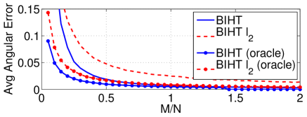
To test the hypothesis that this term is the key differentiator between the algorithms, we implemented BIHT-, a one-sided variation of the BIHT algorithm that enabled a fair comparison of the one-sided objectives (see Section 4.2 for details). We compared both the angular error and Hamming error performance of BIHT and BIHT-. Furthermore, we implemented oracle assisted variations of these algorithms where the true support of the signal is given a priori, i.e., in (14) is replaced by an operator that always selects the true support, and thus the algorithm only needs to estimate the correct coefficient values. The oracle assisted case can be thought of as a “best performance” bound for these algorithms. Using these algorithms, we perform the same experiment detailed at the beginning of the section.
The results are depicted in Figure 4. The angular error behavior of BIHT- is very similar to that of MSP and RSS and underperforms when compared to BIHT. We see the same situation with regards to Hamming error: BIHT finds consistent solutions for the majority of trials, but BIHT- does not.
Thus, the results of this simulation suggest that the one-sided term plays a significant role in the quality of the solution obtained.
One way to explain the performance discrepancy between the two objectives comes from observing the connection between our reconstruction problem and binary classification. As explained previously, in the classification context, the one-sided objective is similar to the hinge-loss, and furthermore, the one-sided objective is similar to the so-called square-loss. Previous results in machine learning have shown that for typical convex loss functions, the minimizer of the hinge loss has the tightest bound between expected risk and the Bayes optimal solution [62] and good error rates, especially when considering robustness to outliers [62, 63]. Thus, the hinge loss is often considered superior to the square loss for binary classification.888Additional “well-behaved” loss functions (e.g., the Huber-ized hinge loss) have been proposed [64] and a host of classification algorithms related to this problem exist [65, 66, 67, 63, 64], both of which may prove useful in the -bit CS framework in the future. One might suspect that since the one-sided -objective is very similar to the hinge loss, it too should outperform other objectives in our context. Understanding why in our context, the geometry of the and objectives results in different performance is an interesting open problem.
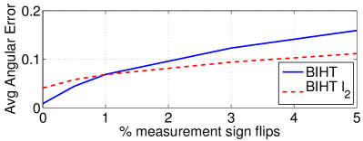
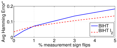
We probed the one-sided / objectives further by testing the two versions of BIHT on noisy measurements. We flipped a number of measurement signs at random in each trial. For this experiment, and are fixed, and we performed 100 trials. We varied the number of sign flips between and of the measurements. The results of the experiment are depicted in Figure 5. We see that for both the angular error in Figure 5(a) and Hamming error in Figure 5(b), that the one-sided objective performs better when there are only a few errors and the one-sided objective performs better when there are significantly more errors. This is expected since the objective promotes sparse errors. This experiment implies that BIHT- (and the other one-sided -based algorithms) may be more useful when the measurements contain significant noise that might cause a large number of sign flips, such as Gaussian noise.
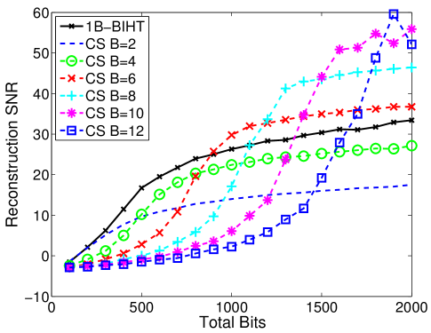
Performance with a fixed bit-budget. In some applications we are interested in reducing the total number of bits acquired due to storage or communication costs. Thus, given a fixed total number of bits, an interesting question is how well -bit CS performs in comparison to conventional CS quantization schemes and algorithms. For the sake of brevity, we give a simple comparison here between the -bit techniques and uniform quantization with Basis Pursuit DeNoising (BPDN) [8] reconstruction. While BPDN is not the optimal reconstruction technique for quantized measurements, it (and its variants such as the LASSO [64]) is considered a benchmark technique for reconstruction from measurements with noise and furthermore, is widely used in practice.
The experiment proceeds as follows. Given a total number of bits and a (uniform) quantization bit-depth (i.e., number of bits per measurement), we choose the number of measurements as , , and the sparsity . The remainder of the experiment proceeds as described earlier (in terms of drawing matrices and signals). For bit depth greater than , we reconstruct using BPDN with an optimal choice of noise parameter and we scale the quantizer to such that signal can take full advantage of its dynamic range.
The results of this experiment are depicted in Figure 6. We see a common trend in each line: lackluster performance until “sufficient” measurements are acquired, then a slow but steady increase in performance as additional measurement are added, until a performance plateau is reached. Thus, since lower bit-depth implies that a larger number of measurements will be used, -bit CS reaches the performance plateau earlier than in the multi-bit case (indeed, the transition point is achieved at a higher number of total bits as the bit-depth is increased). This enables significantly improved performance when the rate is severely constrained and higher bit-rates per measurements would significantly reduce the number of available measurements. For higher bit-rates, as expected from the analysis in [37], using fewer measurements with refined quantization achieves better performance.
It is also important to note that, regardless of trend, the BIHT algorithm performs strictly better than BPDN with bits per measurement and uniform quantization for the parameters tested here. This gain is consistent with similar gains observed in [30, 31]. A more thorough comparison of additional CS quantization techniques with -bit CS is a subject for future study.
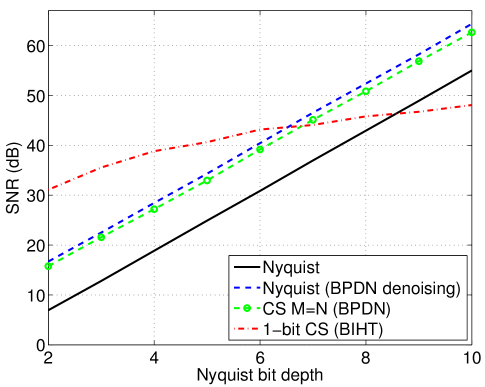
Comparison to quantized Nyquist samples. In our final experiment, we compare the performance of the -bit CS technique to the performance of a conventional uniform quantizer applied to uniform Nyquist-rate samples. Specifically, in each trial we draw a new Nyquist-sampled signal in the same way as in our previous experiments and with fixed and ; however, now the signals are sparse in the discrete cosine transform (DCT) domain. We consider four reconstruction experiments. First, we quantize the Nyquist-rate signal with a bit-depth of bits per time-domain sample (and optimal quantizer scale) and perform linear reconstruction (i.e., we just use the quantized samples as sample values). Second, we apply BPDN to the quantized Nyquist-rate samples with optimal choice of noise parameter, thus denoising the signal using a sparsity model. Third, we draw a new Gaussian matrix with , quantize the measurements to bits, again at optimal quantizer scale, and reconstruct using BPDN. Fourth, we draw a new Gaussian matrix with and compute measurements, quantize to one bit per measurement by maintaining their sign, and perform reconstruction with BIHT. Note that the same total number of bits is used in each experiment.
Figure 7 depicts the average SNR obtained by performing of the above trials. The linear, BPDN, Gaussian measurements with BPDN, and BIHT reconstructions are depicted by solid, dashed, dash-circled, and dash-dotted lines, respectively. The linear reconstruction has a slope of dB/bit-depth, exhibiting a well-known trade-off for conventional uniform quantization. The BPDN reconstruction (without projections) follows the same trend, but obtains an SNR that is at least dB higher than the linear reconstruction. This is because BPDN imposes the sparse signal model to denoise the signal. We see about the same performance with the Gaussian projections at , although it performs slightly worse than without projections since the Gaussian measurements require a slightly larger quantizer range. Similarly to the results in Fig. 6, in low Nyquist bit-depth regimes (), -bit CS achieves a significantly higher SNR than the other two techniques. When , -bit CS is competitive with the BPDN scenario. Thus, for a fixed number of bits, -bit CS is competitive to conventional sampling with uniform quantization, especially in low bit-depth regimes.
6 Discussion
In this paper we have developed a rigorous mathematical foundation for -bit CS. Specifically, we have demonstrated a lower bound on reconstruction error as a function of the number of measurements and the sparsity of the signal. We have demonstrated that Gaussian random projections almost reach this lower bound (up to a log factor) in the noiseless case. This behavior is consistent with and extends existing results in the literature on multibit scalar quantization and 1-bit quantization of non-sparse signals.
We have also introduced reconstruction robustness guarantees through the binary -stable embedding (BSE) property. This property can be thought of as extending the RIP to -bit quantized measurements. To our knowledge, this is the first time such a property has been introduced in the context of quantization. To be able to use this property we showed that random constructions using Gaussian pdf (or more generally using isotropic pdf in the signal space ) generate such embeddings with high probability. This construction class is still very limited compared to the numerous random constructions known for generating RIP matrices. Extending this class with other constructions is an interesting topic for future research.
Using the BSE, we have proven that -bit CS systems are robust to measurement noise added before quantization as well as to signals that are not exactly sparse but compressible.
We have introduced a new -bit CS algorithm, BIHT, that achieves better performance over previous algorithms in the noiseless case. This improvement is due to the enforcement of consistency using a one-sided linear objective, as opposed to a quadratic one. The linear objective is similar to the hinge loss from the machine learning literature.
We remind the reader that the central goal of this paper has been signal acquisition with quantization. As explained previously, one motivation for our work is the development of very high speed samplers. In this case, we are interested in building fast samplers by relaxing the requirements on the primary hardware burden, the quantizer. Such devices are susceptible to noise. Thus, while our noiseless results extend previous -bit quantization results (e.g., see [53] and [51]) to the sparse signal model setting and are of theoretical interest, a major contribution has been the further development of the robust guarantees, even if they produce error rates that seem suboptimal when compared to the noiseless case.
A number of interesting questions remain unanswered. As we discuss in Section 3.2 earlier, we have found that the BSE holds for Gaussian matrices with angular error decay roughly on the order of worse than optimal. One question is whether this gap can be closed with an alternative derivation, or whether it is a fundamental requirement for stability. Another useful pursuit would be to provide a more rigorous understanding of the discrepancy between the performance of the one-sided and objectives. Analysis of the performance behavior might lead to better one-sided functions.
Acknowledgments
Thanks to Rachel Ward for pointing us to the right reference with regards to the lower bound (17) used in Appendix A and recommending several useful articles as well as Vivek Goyal for pointing us to additional prior work in this area. Thanks to Zaiwen Wen and Wotao Yin for sharing some of the data from [32] for our algorithm comparisons, as well as engaging in numerous conversations on this topic. Thanks also to Nathan Srebro for his advice and discussion related to the one-sided penalty comparison and connections to binary classification, and thanks to Amirafshar Moshtaghpour for his correction of a small error in the bounds of Appendix G. Finally, thanks to Yaniv Plan and anomynous reviewers for their useful advices and remarks for improving this paper, and in particular the proof of Theorem 1 with respect to the optimality of the covering.
Appendix A Lemma 1: Intersections of Orthants by Subspaces
While there are available quantization points provided by -bit measurements, a -sparse signal will not use all of them. To understand how effectively the quantization bits are used, we first investigate how the -dimensional subspaces projected from the -dimensional -sparse signal spaces intersect orthants in the -dimensional measurement space, as shown in Fig 1 for and .
We use to denote the maximum number of orthants in dimensions intersected by a -dimensional subspaces. A bound of for is developed in [68, 69]:
| (17) |
For , this simplifies to .
Using we can also derive a simple bound on (17) for . We observe that
Repeating the same argument, we find and finally
| (18) |
using the bound .
While the bound in (17) is tight and holds for subspaces in a general configuration, the closed form simplified bound in (18) can be improved by a factor of (which asymptotically makes no difference in the subsequent development) using the proof we develop in the remainder of this appendix. In addition to the improvement, the proof also provides significant geometrical intuition to the problem.
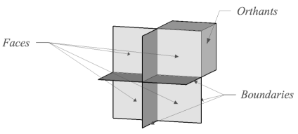
First we define two new elements in the geometry of the problem: orthant boundaries and their faces. Each orthant has boundaries of dimension , defined as the subspace with a coordinate set to 0:
We split each boundary into faces, defined as the set
where is the sign vector of a bordering orthant, and is the boundary in which the face lies. Each face borders two orthants. Note that the faces are -dimensional orthants in the -dimensional boundary subspace. The geometry of the problem in is summarized in Figure 8(a).
Next, we upper bound using an inductive argument that relies on the following two lemmas:
Lemma 6.
If a -dimensional subspace is not the subset of a boundary , then the subspace and boundary do intersect and their intersection is a -dimensional subspace of .
Proof.
We count the dimensions of the relevant spaces. If is not a subset of , then it equals the direct sum , where is also not a subspace of . Since , , and follows.
Lemma 7.
For , a -dimensional subspace that intersects an orthant also non-trivially intersects at least faces bordering that orthant.
Proof.
Consider a -subspace , a point interior to the orthant , and a vector non-parallel to . The following iterative procedure can be used to prove the result:
-
1.
Starting from 0, grow until the set intersects a boundary , say at . It is straightforward to show that as grows, a boundary will be intersected. The point of intersection is in the face . The set is in the orthant .
-
2.
Determine a vector parallel to all the boundaries already intersected and not parallel to , set and iterate from step 1.
A vector can always be found in step 2 for the first iterations since is -dimensional. The vector is parallel to all the boundaries intersected in the previous iterations and therefore always intersects a boundary not intersected before. Therefore, at least distinct faces are intersected.
Lemma 8.
The number of orthants intersected by a -dimensional subspace in an -dimensional space is upper bounded by
Proof.
The main intuition is that since the faces on each boundary are equivalent to orthants in the lower dimensional subspace of the boundary, the maximum number of faces intersected at each boundary is a problem of dimension .
If is contained in one of the boundaries in , the number of orthants of intersected is at most . Since is non-decreasing in and , we can ignore this case in determining the upper bound.
If is not contained in one of the boundaries then Lemma 6 shows that the intersection of with any boundary is a -dimensional subspace in . To count the faces of intersected by we use the observation in the definition of faces above, that each face is also an orthant of . Therefore, the maximum number of faces of intersected is a recursion of the same problem in lower dimensions, i.e., is upper bounded by . Since there are boundaries in , it follows that the number of faces in intersected by is upper bounded by .
Using Lemma 7 we know that for an orthant to be intersected, at least faces adjacent to it should be intersected. Since each face is adjacent to two orthants, the total number of orthants intersected cannot be greater than twice the number of faces intersected divided by :
| (19) |
To complete the induction we use for all ; for the subspace is a line through the origin, which can intersect only two orthants999We recall that, from the definition (4), two different orthants have an empty intersection.. This leads to:
Appendix B Theorem 1: Distributing Signals to Quantization Points
To prove Theorem 1 we consider how the available quantization points optimally cover the set of signals . This set corresponds to the union of -dimensional unit spheres , each being associated to one support taken amongst the available -length supports of . The cover should be optimal with respect to the worst case distance, denoted by , of any point in to its closest quantization point. Our goal is to determine a lower bound on the best-case we can achieve.
Unfortunately, determining the optimal cover of is not straightforward. For instance, optimally covering each individually does not produce an optimal cover for their union. Indeed, at the intersection of different -dimensional spheres in there are -sparse signals, with different support, very close to each other. A single quantization point in could be close to all those signals, whereas independent cover of each would have to use a different quantization point to represent the signals on each sphere in that intersection.
Thus, instead of determining the optimal cover of , we establish a lower bound on required to cover a subset of using the same number of points. A cover of with a smaller would not be possible, since that would also cover with the same or smaller . Therefore, this establishes a lower bound for the cover of . To establish the bound, we pick such that the neighborhood around the intersection of the balls is not included. Specifically, we pick
In other words, we pick the subset of each -ball, such that all the nonzero coordinates of the signals in the subset are greater than . The union of those subsets for all possible supports comprises . This choice ensures that any signal has distance at least from any signal in any other , and therefore both cannot be close to a common quantization point in with distance from each. Notice that is non empty as soon as .
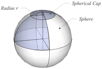
With this choice of , an optimal covering can be obtained by merging the optimal coverings of each for . For an optimal covering of distance , each of the elements in should belong to some ball of radius centered at the quantization point. Thus, each quantization point and its corresponding -ball should cover as large an area of as possible. This is achieved when the quantization point is on , and the intersection of the ball with is a spherical cap of radius [70]. Thus, for the spherical caps to cover , the total area of all spherical caps in the cover should be greater than the area of . Furthermore, since the overall cover of is composed of separate cover of each , the total area of all spherical caps used for the cover should be greater than the area of .
Therefore, since quantization points and corresponding spherical caps are available, according to Lemma 1 and Corollary 1, to cover subsets of -spheres, as described above, the cover should satisfy
| (20) |
where denotes the rotationally invariant area measure the -sphere and denotes the surface of a spherical cap of radius .
To determine the smallest satisfying (20), we thus need to measure the set . Choosing one we have since the sets () are disjoint with identical area. We first show that
| (21) |
where is a -dimensional sphere in . Note that this bound is tight at two ends: at where (almost everywhere) and at for which .
To prove (21) we assume without loss of generality and consider and . We define the intersection with the positive orthant . By symmetry, since there are orthants in . As described in [70], the ratio between the measure of and the one of the full sphere equals the ratio between the volume occupied by a cone formed by in the unit ball and the volume of this ball, i.e.,
| (22) |
where is the Lebesgue measure in and is the portion of the cone (with apex on the origin and restricted to ) formed by the subset . The geometry of our problem is made clear in Figure 9.
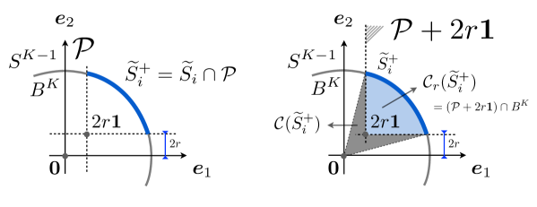
To measure the volume of , writing , we first define the set
also shown in the figure, which is non-empty for . Since and , it is straightforward to show that , and therefore the measure of is a lower bound to the measure of . Furthermore, by the translation invariance of ,
where is the unit ball centered on . Setting it follows that for any , . Consequently, and . Therefore, the measure of the positive orthant of a -ball with radius lower bounds the measure of .
Appendix C Theorem 2: Optimal Performance via Gaussian Projections
To prove Theorem 2, we follow the procedure given in [48, Theorem 3.3]. We begin by restricting our analysis to the support set with , and thus we consider vectors that lie on the (sub) sphere . We remind the reader that is the ball of unit norm vectors of Euclidean distance around , and we write as in Section 3.2.
Let us fix a radius to be precised later. The sphere can be covered with a finite set of no more than points such that, for any , there exists a with [16].
Using the notation defined in Sec. 3.1, given a vector and two distinct points and in , we have that
from Lemma 9 (given in Appendix D). Since for all and
we can write for any
By setting (and reversing the inequality), we obtain
Thus, for different random vectors arranged in , and for the associated mapping defined in (3), we get
In other words, we have found a bound on the probability that two vectors’ measurements are consistent, even if their Euclidean distance is greater than , but only for vectors in the restricted (sub) sphere . Now we seek to cover the rest of the space (unit norm -sparse signals).
Since there are no more than pairs of distinct points in , we find
To obtain the final bound, we observe that any pair of unit -sparse vectors and in belongs to some with and . There are no more than of such sets , and thus setting above yields
where the second inequality follows from . By upper bounding this probability by and solving for , we obtain
Since , we have that , and thus the previous relation is then satisfied when
Appendix D Lemma 3: Concentration of Measure for -Balls
Since is fixed with size , proving Lemma 3 amounts to showing that, for any fixed and , given a Gaussian matrix , the mapping defined as , and for any fixed , we have
where, in this case, for any .
Given and , the quantity is the sum , where stands for the component of . For one index
and therefore
Of course, the occurrence of () means that all vector pairs taken separately in and have consistent (or respectively, inconsistent) measurements on the sensing component . More precisely, since , are binary random variables such that and independently of , where the probabilities and are defined by
In summary, and are binomially distributed with trials and probability of success and , respectively. Furthermore, we have that and , thus by the Chernoff-Hoeffding inequality,
This indicates that with a probability higher than , we have
The final result follows by lower bounding and as in Lemma 9.
Lemma 9.
Given and two unit vectors , we have
| (23) | ||||
| (24) |
Proof of Lemma 9.
We begin by introducing some useful properties of Gaussian vector distribution. If , the probability that is simply the measure of with respect to the standard Gaussian density , i.e.,
with . It may be easier to perform this integration over a hyper-spherical set of coordinates measured in a basis defined by the vectors and . This is possible since the pdf is rotationally invariant.
Specifically, we consider the canonical basis of where, by using the cross product in , , and , while the other vectors are defined arbitrarily for completing the basis. In this system, the “” plane is equivalent to the plane spanned by and . Moreover, any vector can be represented by the spherical coordinates where , corresponds to the vector angles in each dimension, and being the angle formed by the projection of in the “” plane with .
The change of coordinates between the Cartesian and the spherical representations of in is then defined as , , …, , and , while, conversely, , , …, , and .101010This change of coordinates can be very convenient. For instance, the proof of Lemma 2 relies on the computation , since for (almost) all , and live in the two different subvolumes determined by the plane [57, 58].
We now seek a lower bound on . Computing this probability amounts to estimating
where is the set of all vectors such that its inner product with and result in different signs.
Note that if , then since . This non-empty intersection is avoided when . Furthermore, since for any , this occurs if .
The remainder of the proof is devoted to finding an appropriate way to integrate the set . To this end, we begin by demonstrating that estimating can be simplified with the following equivalence (proved just after the completion of the proof of Lemma 9).
Lemma 10.
The set is equal to the set
where is the orthogonal projection on the plane .
Using the hyper spherical coordinate system developed earlier and denoting the angle by , membership in can be expressed as
| (R1) | |||
| (R2) | |||
| (R3) |
Indeed, requirement (R1) enforces , while (R2) and (R3) are direct translations of the requirements that and , with .
We are now ready to integrate to find :
with if and 0 else, for some , and .
However,
and , since for any . Consequently,
with and knowing that since
Using the fact that , we obtain , and thus
If we want a meaningful bound for , then we must have . Therefore, as soon as the lower bound is positive, the aforementioned condition always holds.
The lower bound for is obtained similarly. It is straightforward to show that , with . Lower bounding as for , the only difference occurring with the integral on given by
Therefore, the lower bound of amounts to change in the one of , which provides the result.
Proof of Lemma 10.
If , there is nothing to prove. Therefore and if belongs to either or , we must have . It is also sufficient to work on the restriction of and to unit vectors.
(i) : By contradiction, let us assume that but . Without any loss of generality, and . Since , there exist two vectors and such that . If and , then, since and by continuity of the inner product, there exist a such that with . Therefore, and, by definition of the orthogonal projection, which is a contradiction. If and , we apply the same reasoning on and . Therefore, .
(ii) : If with , we have either or . Let us say that . Then, for , . However, and , leading to , which is a contradiction.
Appendix E Theorem 3: Gaussian Matrices Provide BSEs
The strategy for proving Theorem 3 will be to count the number of pairs of -sparse signals that are Euclidean distance apart. We will then apply the concentration results of Lemma 3 to demonstrate that the angles between these pairs are approximately preserved. We specifically proceed by focusing on a single -dimensional subspace (intersected with the unit sphere) and then by applying a union bound to account for all possible subspaces.
Let be an index set of size , be the sphere of unit vectors with support . We first use again the fact that the sphere can be -covered by a finite set of points . That is, for any , there exists a such that [16]. Note that the size of is bounded by .
Let be the matrix formed by the columns of indexed by and note that . Given , for all pairs of points , we have
| (25) |
This follows from Lemma 3 with , since is a Gaussian matrix and by invoking the union bound, since there are such pairs .
The bound (25) can be extended to all possible index sets of size via the union bound. Specifically, for all and all pairs of points , we have now jointly
| (26) |
since there are no more than possible .
We can reformulate this last result as follows. Let us take any pair of points on the sphere such that their joint support has a size . We have obviously . Taking the covering set defined for , there exist two points such that and . From (26), with a probability exceeding , we have
| (27) |
To obtain our final bound, consider that implies that , and can be similarly bounded. Thus, and , and (27) becomes
| (28) |
Let us define the probability of failure as where , and set and . Solving for , we finally get that with a probability bigger than if
Since , we have that , and thus the previous relation is satisfied if
Appendix F Lemma 4: Stability with Measurement Noise
In Lemma 4, since , each follows a Gaussian distribution , and furthermore, since we have independent additive noise, follows the Gaussian distriubtion .
We begin by bounding the probability that any noisy measurement has a different sign than the original corresponding measurement , i.e., we bound . This quantity is interesting since follows a Binomial distribution with trials and probability of success and thus we also have .
To solve for the bound, we compute
with the pdf . This leads to
where denotes the tail integral of the standard Gaussian distribution which is bounded by for (see for instance [71, Eq. (13.48)]).
Thus, we have and, by applying the Chernoff-Hoeffding inequality to the distribution of ,
which proves the lemma.
Appendix G Asymptotic bound on in Theorems 2 and 3
Both Theorem 2 and Theorem 3 provide guarantees on the worst-case error of the form
| (29) |
for some exponent , and for given constants .
In this appendix we show that, considering fixed, the relation (29) implies
| (30) |
asymptotically in and . Notice that, up to a redefinition and , it is sufficient to prove the relation for . We also define .
First, we consider fixed and show . Let us assume this is not the case, i.e., for all , and all , there exists a ratio such that . Therefore,
Thus (29) becomes
Using , this last inequality becomes
| (31) |
For fixed and , and since we reasonably have , the parameters and can always be selected so that . In this case, (31) implies . Taking , which is still compatible with the selection of and above, leads to a contradiction. Thus for fixed .
Next, we assume varies and is fixed, and show that . We again restrict the analysis to . Now we assume for all and all , there is an such that . Therefore, and (29) becomes
Since and are fixed and we have , the parameters and can be selected so that , that implies . Taking leads to a contradiction and completes the proof.
References
- [1] E. Candès, “Compressive sampling,” in Proc. Int. Congress Math., Madrid, Spain, Aug. 2006.
- [2] D. Donoho, “Compressed sensing,” IEEE Trans. Inf. Theory, vol. 6, no. 4, pp. 1289–1306, 2006.
- [3] J. Tropp, J. Laska, M. Duarte, J. Romberg, and R. Baraniuk, “Beyond Nyquist: Efficient sampling of sparse, bandlimited signals,” IEEE Trans. Inf. Theory, vol. 31, no. 1, pp. 520–544, 2010.
- [4] M. Duarte, M. Davenport, D. Takhar, J. Laska, T. Sun, K. Kelly, and R. Baraniuk, “Single-pixel imaging via compressive sampling,” IEEE Sig. Proc. Mag., vol. 25, no. 2, pp. 83–91, 2008.
- [5] B. K. Natarajan, “Sparse approximate solutions to linear systems,” SIAM J. on Comp., vol. 24, pp. 227, 1995.
- [6] S. S. Chen, D.L. Donoho, and M.A. Saunders, “Atomic decomposition by basis pursuit,” SIAM J. on Sci. Comp., vol. 20, no. 1, pp. 33–61, 1998.
- [7] E. Candès, “The restricted isometry property and its implications for compressed sensing,” Comptes rendus de l’Académie des Sciences, Série I, vol. 346, no. 9-10, pp. 589–592, 2008.
- [8] E. Candès, J. Romberg, and T. Tao, “Stable signal recovery from incomplete and inaccurate measurements,” Comm. Pure and Appl. Math., vol. 59, no. 8, pp. 1207–1223, 2006.
- [9] E. T. Hale, W. Yin, and Y. Zhang, “A fixed-point continuation method for regularized minimization with applications to compressed sensing,” in Rice University Technical Report TR07-07, 2007.
- [10] M. A. T. Figueiredo, R. D. Nowak, and S. J. Wright, “Gradient projection for sparse reconstruction: Application to compressed sensing and other inverse problems,” IEEE J. of Sel. Top. in Sig. Proc., Sept. 2007.
- [11] E. Candès and T. Tao, “The Dantzig selector: Statistical estimation when is much larger than ,” Annals of Statistics, vol. 35, no. 6, pp. 2313–2351, 2007.
- [12] D. Needell and R. Vershynin, “Uniform uncertainty principle and signal recovery via regularized orthogonal matching pursuit,” Found. Comput. Math., vol. 9, no. 3, pp. 317–334, 2009.
- [13] D. Needell and J. Tropp, “CoSaMP: Iterative signal recovery from incomplete and inaccurate samples,” Appl. Comput. Harmon. Anal., vol. 26, no. 3, pp. 301–321, 2009.
- [14] T. Blumensath and M. Davies, “Iterative hard thresholding for compressive sensing,” Appl. Comput. Harmon. Anal., vol. 27, no. 3, pp. 265–274, 2009.
- [15] P. J. Huber, “Robust regression: Asymptotics, conjectures, and Monte Carlo,” Statistics, vol. 1, pp. 799–821, 1973.
- [16] R. Baraniuk, M. Davenport, R. DeVore, and M. Wakin, “A simple proof of the restricted isometry property for random matrices,” Const. Approx., vol. 28, no. 3, pp. 253–263, 2008.
- [17] M. Davenport, Random observations on random observations: Sparse signal acquisition and processing, Ph.d. thesis, Rice University, Aug. 2010.
- [18] J. Romberg, “Compressive sensing by random convolution,” SIAM J. Imaging Sciences, 2009.
- [19] J. Tropp, M. Wakin, M. Duarte, D. Baron, and R. Baraniuk, “Random filters for compressive sampling and reconstruction,” in Proc. IEEE Int. Conf. Ac., Speech, Sig. Proc. (ICASSP), Toulouse, France, May 2006.
- [20] L. Jacques, P. Vandergheynst, A. Bibet, V. Majidzadeh, A. Schmid, and Y. Leblebici, “CMOS compressed imaging by random convolution,” in Proc. IEEE Int. Conf. Ac., Speech, Sig. Proc. (ICASSP), Taipei, Taiwan, Apr. 2009.
- [21] L. Jacques, D. Hammond, and M. Fadili, “Dequantizing compressed sensing: When oversampling and non-gaussian contraints combine,” IEEE Trans. Inf. Theory, vol. 57, no. 1, pp. 559–571, 2011.
- [22] J. Laska, P. Boufounos, M. Davenport, and R. Baraniuk, “Democracy in action: Quantization, saturation, and compressive sensing,” to appear in App. Comp. and Harm. Anal. (ACHA), 2011.
- [23] W. Dai, H. Pham, and O. Milenkovic, “Distortion-rate functions for quantized compressive sensing,” in IEEE Inform. Theory Workshop on Networking and Inform. Theory (ITW), Jun. 2009.
- [24] A. Zymnis, S. Boyd, and E. Candès, “Compressed sensing with quantized measurements,” IEEE Signal Processing Letters, vol. 17, no. 2, Feb. 2010.
- [25] J. Sun and V. Goyal, “Quantization for compressed sensing reconstruction,” in Proc. Sampling Theory and Applications (SampTA), Marseille, France, May 2009.
- [26] G. Gray and G. Zeoli, “Quantization and saturation noise due to analog-to-digital conversion,” IEEE Trans. Aerospace and Elec. Systems, vol. 7, no. 1, pp. 222–223, 1971.
- [27] R. Walden, “Analog-to-digital converter survey and analysis,” IEEE J. Selected Areas in Comm., vol. 17, no. 4, pp. 539–550, 1999.
- [28] B. Le, T. W. Rondeau, J. H. Reed, and C. W. Bostian, “Analog-to-digital converters,” IEEE Sig. Proc. Mag., Nov. 2005.
- [29] P. Boufounos, “Reconstruction of sparse signals from distorted randomized measurements,” in Proc. IEEE Int. Conf. Ac., Speech, Sig. Proc. (ICASSP), Dallas, TX, Mar. 2010.
- [30] P. Boufounos and R. Baraniuk, “1-bit compressive sensing,” in Proc. Conf. Inf. Sc. Sys. (CISS), Princeton, NJ, Mar. 2008.
- [31] P. Boufounos, “Greedy sparse signal reconstruction from sign measurements,” in Proc. Asilomar Conf. on Signals Systems and Comput., Asilomar, California, Nov. 2009.
- [32] J. Laska, Z. Wen, W. Yin, and R. Baraniuk, “Trust, but verify: Fast and accurate signal recovery from 1-bit compressive measurements,” IEEE Trans. on Sig. Proc., vol. 59, no. 11, pp. 5289–5301, 2011.
- [33] Y. Plan and R. Vershynin, “Dimension reduction by random hyperplane tessellations,” preprint, arXiv:1111.4452, 2011.
- [34] Y. Plan and R. Vershynin, “One-bit compressed sensing by linear programming,” preprint, arXiv:1109.4299, 2011.
- [35] Y. Plan and R. Vershynin, “Robust 1-bit compressed sensing and sparse logistic regression: A convex programming approach,” preprint, arXiv:1202.1212, 2012.
- [36] P. Boufounos, Quantization and erasures in frame representations, Ph.D. thesis, MIT EECS, Cambridge, MA, Jan. 2006.
- [37] P. Boufounos and R. Baraniuk, “Quantization of sparse representations,” in Proc. data compression conference (DCC), Mar. 2007, p. 378.
- [38] J. Z. Sun and V. K. Goyal, “Optimal quantization of random measurements in compressed sensing,” in International Symposium on Information Theory (ISIT), June 2009.
- [39] N. Thao and M. Vetterli, “Reduction of the MSE in -times oversampled A/D conversion to ,” IEEE Trans. Signal Processing, vol. 42, no. 1, pp. 200–203, 2994.
- [40] V. K. Goyal, M. Vetterli, and N. Thao, “Quantized overcomplete expansions in : Analysis, synthesis, and algorithms,” IEEE Trans. Inf. Theory, vol. 44, no. 1, pp. 16–31, 1998.
- [41] P. M. Aziz, H. V. Sorensen, and J. Van Der Spiegel, “An overview of Sigma-Delta converters,” IEEE Sig. Proc. Mag., vol. 13, no. 1, pp. 61–84, Jan. 1996.
- [42] N. T. Thao, “Vector quantization analysis of modulation,” IEEE Trans. Signal Processing, vol. 44, no. 4, pp. 808–817, Apr. 1996.
- [43] J. C. Candy and G. C. Temes, Eds., Oversampling Delta-Sigma converters, IEEE Press, 1992.
- [44] J. J. Benedetto, A. M. Powell, and O. Yilmaz, “Sigma-delta quantization and finite frames,” IEEE Trans. Inf. Theory, vol. 52, no. 5, pp. 1990–2005, May 2006.
- [45] P. Boufounos and A. V. Oppenheim, “Quantization noise shaping on arbitrary frame expansions,” EURASIP J. App. Sig. Proc., vol. 2006, ID 53807, 12 pages, 2006.
- [46] P. Boufounos and R. Baraniuk, “Sigma delta quantization for compressive sensing,” in Proc. SPIE Waveletts XII. Proc. of SPIE vol. 6701, 670104, San Diego, CA, Aug. 2007.
- [47] S. Gunturk, A. Powell, R. Saab, and O. Yülmaz, “Sobolev duals for random frames and sigma-delta quantization of compressed sensing measurements,” preprint, Feb. 2010.
- [48] P. Boufounos, “Universal rate-efficient scalar quantization,” IEEE Trans. Inf. Theory, vol. 3, no. 58, pp. 1861–1872, 2012.
- [49] C.S. Güntürk, “One-bit sigma-delta quantization with exponential accuracy,” Communications on Pure and Applied Mathematics, vol. 56, no. 11, pp. 1608–1630, 2003.
- [50] P. T. Boufounos, “Hierarchical distributed scalar quantization,” in Proc. Int. Conf. Sampling Theory and Applications (SampTA), Singapore, May 2-6 2011.
- [51] H. Q. Nguyen, V.K. Goyal, and L.R. Varshney, “Frame permutation quantization,” Applied and Computational Harmonic Analysis (ACHA), Nov. 2010.
- [52] P. Indyk and R. Motwani, “Approximate nearest neighbors: towards removing the curse of dimensionality,” in Proceedings of the thirtieth annual ACM symposium on Theory of computing. ACM, 1998, pp. 604–613.
- [53] A. Andoni, M. Datar, N. Immorlica, P. Indyk, and V. Mirrokni, “Locality-sensitive hashing scheme based on p-stable distributions,” Nearest neighbor methods in learning and vision: Theory and practice (book), 2006.
- [54] A. Andoni and P. Indyk, “Near-optimal hashing algorithms for approximate nearest nieghbor in high dimensions,” Commun. ACM, vol. 51, no. 1, pp. 117–122, 2008.
- [55] M. Raginsky and S. Lazebnik, “Locality-sensitive binary codes from shift-invariant kernels,” The Neural Information Processing Systems, vol. 22, 2009.
- [56] M. Bridson, “Geometric and combinatorial group theory,” in The Princeton companion to mathematics, T. Gowers, J. Barrow-Green, and I. Leader, Eds., chapter IV.10, pp. 431–447. Princeton Univ. Press, 2008.
- [57] M. Goemans and D. Williamson, “Improved approximation algorithms for maximum cut and satisfiability problems using semidefinite programming,” Journ. ACM, vol. 42, no. 6, pp. 1145, 1995.
- [58] S. Shariati, L. Jacques, F. X. Standaert, B. Macq, M. A. Salhi, and P. Antoine, “Randomly driven fuzzy key extraction of unclonable images,” in IEEE Int. conf. on image proc. (ICIP), 2010.
- [59] A. Gupta, B. Recht, and R. Nowak, “Sample complexity for 1-bit compressed sensing and sparse classification,” in Proc. Intl. Symp. on Information Theory (ISIT), 2010.
- [60] T. Blumensath, “Compressed sensing with nonlinear observations,” preprint, 2010.
- [61] T. Hastie, R. Tibshirani, and J. Friedman, The elements of statistical learning, Springer Series in Statistics, 2nd edition, Feb. 2009.
- [62] L. Rosasco, E. De Vito, A. Caponnetto, M. Piana, and A. Verri, “Are loss functions all the same?,” Neural Comp., vol. 16, no. 5, pp. 1063–1076, Mar. 2004.
- [63] N. Srebro, K. Sridharan, and A. Tewari, “Smoothness, low-noise, and fast rates,” in Advances in Neural Information Processing Systems (NIPS), Dec. 2010.
- [64] R. Tibshirani, “Regression shrinkage and selection via the lasso,” Royal Statistical Society. Series B (Methodological), pp. 267–288, 1996.
- [65] O. Bartlett, Y. Freund, W. S. Lee, and R. E. Schapire, “Boosting the margin: a new explanation for the effectiveness of voting methods,” Annals of Statistics, vol. 26, no. 5, pp. 1651–1686, 1998.
- [66] G. Ratsch and M. Warmuth, “Efficient margin maximizing with boosting,” The J. of Machine Learning Research, vol. 6, Dec. 2005.
- [67] A. Blum, On-line algorithms in machine learning, vol. 1442/1998 of Lecture Notes in Computer Science, Springer, 1998.
- [68] T. M. Cover, “Geometrical and statistical properties of systems of linear inequalities with applications in pattern recognition,” IEEE Trans. on Electronic Comp., vol. 3, pp. 326–334, Jun. 1965.
- [69] L. Flatto, “A new proof of the transposition theorem,” Proc. American Mathematical Society, vol. 24, no. 1, pp. 29–31, jan 1970.
- [70] K. Ball, “An elementary introduction to modern convex geometry,” in Flavors of Geometry, Silvio Levy, Ed., vol. 31 of MSRI Publications, pp. 1–58. Cambridge University Press, Cambridge, UK, 1997.
- [71] N. Johnson, S. Kotz, and N. Balakrishnan, Continuous univariate distributions, vol. 1, Wiley, 1994.