The WiggleZ Dark Energy Survey: the growth rate of cosmic structure since redshift
Abstract
We present precise measurements of the growth rate of cosmic structure for the redshift range , using redshift-space distortions in the galaxy power spectrum of the WiggleZ Dark Energy Survey. Our results, which have a precision of around in four independent redshift bins, are well-fit by a flat CDM cosmological model with matter density parameter . Our analysis hence indicates that this model provides a self-consistent description of the growth of cosmic structure through large-scale perturbations and the homogeneous cosmic expansion mapped by supernovae and baryon acoustic oscillations. We achieve robust results by systematically comparing our data with several different models of the quasi-linear growth of structure including empirical models, fitting formulae calibrated to N-body simulations, and perturbation theory techniques. We extract the first measurements of the power spectrum of the velocity divergence field, , as a function of redshift (under the assumption that where is the galaxy overdensity field), and demonstrate that the WiggleZ galaxy-mass cross-correlation is consistent with a deterministic (rather than stochastic) scale-independent bias model for WiggleZ galaxies for scales Mpc-1. Measurements of the cosmic growth rate from the WiggleZ Survey and other current and future observations offer a powerful test of the physical nature of dark energy that is complementary to distance-redshift measures such as supernovae and baryon acoustic oscillations.
keywords:
surveys, large-scale structure of Universe, cosmological parameters1 Introduction
**footnotetext: E-mail: cblake@astro.swin.edu.auRecent cosmological observations have revealed significant gaps in our understanding of the physics of the Universe. A set of measurements including the anisotropies of the Cosmic Microwave Background radiation, the shape of the clustering power spectrum of galaxies, the brightness of distant supernovae and the projected scales of baryon acoustic oscillations have indicated the presence of a “dark energy” component which is propelling the cosmic expansion into a phase of acceleration (for recent results see Komatsu et al. 2009, Reid et al. 2009, Percival et al. 2010, Guy et al. 2010).
The physical nature of dark energy is not yet understood. Several explanations have been put forward including the presence of smoothly-distributed energy such as a cosmological constant or a quintessence scalar field, a large-scale modification to Einstein’s theory of General Relativity, or the effects of spatially-varying curvature in an inhomogeneous Universe. Further observational data is required to distinguish clearly between the subtly-varying predictions of these very different physical models (e.g., Linder 2005, Wang 2008, Wiltshire 2009).
One of the most important observational datasets for addressing this issue is the large-scale structure of the galaxy distribution. The clustering within this distribution arises through a process of gravitational instability which acts to amplify primordial matter fluctuations. The growth rate of this structure with time is a key discriminant between cosmological models (e.g., Linder & Jenkins 2003, Linder & Cahn 2007, Nesseris & Perivolaropoulos 2008). Two different physical dark energy scenarios with the same background cosmic expansion generally produce different growth rates of perturbations, hence growth measurements are able to discriminate between models that are degenerate under geometric tests (Davis et al. 2007, Rubin et al. 2009).
The growth of cosmic structure is driven by the motion of matter, for which galaxies act as “tracer particles”. These flows imprint a clear observational signature in galaxy surveys, known as redshift-space distortions, because the galaxy redshift is generated by not only the background cosmic expansion but also the peculiar velocity tracing the bulk flow of matter (Kaiser 1987, Hamilton 1998). As a consequence the 2-point statistics of the galaxy distribution are anisotropic on large scales, where the amplitude of the anisotropy is related to the velocity of the bulk flow and hence to the growth rate of structure.
Many previous galaxy surveys have measured this anisotropy employing either the galaxy correlation function or power spectrum. In the relatively local Universe, exquisite studies at redshift have been undertaken using data from the 2-degree Field Galaxy Redshift Survey (2dFGRS; Peacock et al. 2001, Hawkins et al. 2003, Percival et al. 2004) and the Sloan Digital Sky Survey (SDSS; Tegmark et al. 2004). The SDSS Luminous Red Galaxy (LRG) sample enabled these measurements to be extended to somewhat higher redshifts (Tegmark et al. 2006, Cabre & Gaztanaga 2009, Okumura et al. 2008). Noisier results have been achieved at greater look-back times up to by surveys mapping significantly smaller cosmic volumes such as the 2dF-SDSS LRG and Quasar survey (2SLAQ; da Angela et al. 2008) and the VIMOS-VLT Deep Survey (VVDS; Guzzo et al. 2008).
The current observational challenge is to map the intermediate-redshift Universe with surveys of comparable statistical power to 2dFGRS and SDSS, so that accurate growth rate measurements can be extracted across the full (hypothesized) redshift range for which dark energy dominates the cosmic dynamics. In order to achieve this goal we have constructed the WiggleZ Dark Energy Survey (Drinkwater et al. 2010), a new large-scale spectroscopic galaxy redshift survey, using the multi-object AAOmega fibre spectrograph at the m Australian Astronomical Telescope. The survey, which began in August 2006, targets UV-selected star-forming emission-line galaxies in several different regions around the sky and at redshifts . By covering a total solid angle of deg2 the WiggleZ Survey maps two orders of magnitude more cosmic volume in the Universe than previous galaxy redshift surveys. This paper presents the current measurements of the growth rate of structure using the galaxy power spectrum of the survey. The dataset will also permit many other tests of the cosmological model via baryon acoustic oscillations, the Alcock-Pacyznski effect, higher-order clustering statistics and topological descriptors of the density field.
The improving statistical accuracy with which redshift-space distortions may be measured by observational datasets requires that the theoretical modelling of the data also advances. Recent reviews of this topic have been provided by Percival & White (2009) and Song & Percival (2009). In the linear clustering regime, in the large-scale limit, the theory is well-understood (Kaiser 1987, Hamilton 1998). However, both simulations and observations have demonstrated that linear theory is a poor approximation across a wide range of quasi-linear scales encoding a great deal of clustering information (e.g. Jennings et al. 2011, Okumura et al. 2011). The blind application of linear-theory modelling to current surveys would therefore result in a significant systematic error in the extraction of the growth rate and a potential mis-diagnosis of the physical nature of dark energy.
Various methodologies have been employed for extending the modelling of redshift-space distortions to quasi-linear and non-linear scales. The classical approach – the so-called “streaming model” (e.g. Hatton & Cole 1998) – modulates the linear theory clustering with an empirical damping function characterized by a variable parameter, which is marginalized over when extracting the growth rate. This model has provided an acceptable statistical fit to many previous datasets, but the lack of a strong physical motivation for the empirical function could lead to systematic errors when the model is confronted by high-precision data.
In this paper we consider two alternatives. Firstly, quasi-linear redshift-space distortions can be modelled by various physically-motivated perturbation theory schemes (for recent reviews see Nishimichi et al. 2009; Carlson, White & Padmanabhan 2010). Given that the accuracy of some current perturbation techniques breaks down at a particular quasi-linear scale, leading to potentially large discrepancies at smaller scales, the range of validity of these models must be carefully considered. The second approach is to use numerical N-body simulations to produce fitting formulae for the density and velocity power spectra (Smith et al. 2003, Jennings et al. 2011), which enables models to be established across a wider range of scales. The main concern of this approach is that these fitting formulae may only be valid for the subset of cosmologies and galaxy formation models in which they were derived (an important point given the unknown nature of dark energy).
A further significant issue in the modelling of redshift-space distortions in the galaxy distribution is the “galaxy bias” relation by which galaxies trace the matter overdensities that drive the velocities (e.g., Cole & Kaiser 1989). The typical assumption of a local, linear, deterministic bias, for which there is a good physical motivation on large scales (Scherrer & Weinberg 1998), may break down in the case of precise measurements of the clustering pattern on quasi-linear scales (Swanson et al. 2008), also potentially leading to systematic errors in growth rate fits. In this study we consider the introduction of stochasticity to the bias relation by varying the galaxy-mass cross-correlation (Dekel & Lahav 1999). We note that further studies of the WiggleZ dataset involving the bispectrum, 3-point correlation function, galaxy halo occupation distribution and comparison with numerical simulations will yield further constraints on the form of galaxy bias.
The aim of this paper is to use the existing range of redshift-space distortion models and galaxy power spectra from the WiggleZ survey to derive measurements of the growth rate across the redshift range that are robust against modelling systematics. We assume throughout a cosmological model consistent with the analysis of the latest measurements of the CMB by the Wilkinson Microwave Anisotropy Probe (Komatsu et al. 2009): a flat Universe described by General Relativity with matter density , cosmological constant , baryon fraction , Hubble parameter , primordial scalar index of fluctuations and total fluctuation amplitude . In addition to providing a good description of the temperature and polarization fluctuations in the CMB, this model yields a good fit to distance measurements from supernovae and baryon acoustic oscillations (Guy et al. 2010, Percival et al. 2010). In this paper we test if the same model also predicts the observed growth rate of structure. Future studies will explore simultaneous fits to these datasets using different dark energy models.
The layout of this paper is as follows: in Section 2 we present the measurements of the various observational statistics quantifying the anisotropic power spectrum. Section 3 summarizes the current theory of redshift-space distortions in Fourier space and introduces in more detail the models we will fit to the data. In Section 4 we carry out the parameter fitting focussing on the growth rate and the galaxy-mass cross-correlation. Section 5 presents an analysis of the moments of the power spectrum and extraction of the power spectrum of the velocity divergence field, and Section 6 lists our conclusions.
2 Measurements
2.1 Sample
The WiggleZ Dark Energy Survey at the Australian Astronomical Telescope (Drinkwater et al. 2010) is a large-scale galaxy redshift survey of bright emission-line galaxies mapping a cosmic volume of order 1 Gpc3 over redshift . The survey, which began in August 2006 and is scheduled to finish in January 2011, will obtain of order redshifts for UV-selected galaxies covering of order 1000 deg2 of equatorial sky, using the AAOmega spectrograph (Sharp et al. 2006). The survey design is driven by the scientific goal of measuring baryon acoustic oscillations in the galaxy power spectrum at a significantly higher redshift than existing surveys. The target galaxy population is selected from UV imaging by the Galaxy Evolution Explorer (GALEX) satellite, matched with optical data from the Sloan Digital Sky Survey (SDSS) and Red Cluster Sequence survey (RCS2; Gilbank et al. 2011) to provide an accurate position for fibre spectroscopy. Full details about the survey design, execution and modelling are provided by Blake et al. (2009), Drinkwater et al. (2010) and Blake et al. (2010).
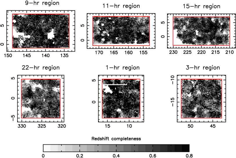
In this paper we analyze a subset of the WiggleZ sample assembled up to the end of the 10A semester (May 2010). We include data from six survey regions – the 9-hr, 11-hr, 15-hr, 22-hr, 1-hr and 3-hr regions – in the redshift range , which together constitute a total sample of galaxies. Figure 1 displays the distribution in right ascension and declination of the analyzed sample for the six survey regions, where the greyscale level corresponds to the relative redshift completeness. We divided the sample into four redshift slices of width in order to map the evolution of the growth rate with redshift. The effective redshifts at which the clustering pattern was measured in each of these slices (evaluated using equation 44 of Blake et al. 2010) were . The numbers of galaxies analyzed in each redshift slice were .
2.2 Power spectrum estimation
We estimated the two-dimensional galaxy power spectrum in four redshift slices for each of the six WiggleZ survey regions using the direct Fourier methods introduced by Feldman, Kaiser & Peacock (1994; FKP). Our methodology is fully described in Section 3.1 of Blake et al. (2010); we give a brief summary here. Firstly we mapped the angle-redshift survey cone into a cuboid of co-moving co-ordinates using a fiducial flat CDM cosmological model with matter density . We gridded the catalogue in cells using nearest grid point assignment ensuring that the Nyquist frequencies in each direction were much higher than the Fourier wavenumbers of interest (we corrected the power spectrum measurement for the small bias introduced by this gridding using the method of Jing 2005). We then applied a Fast Fourier Transform to the grid. The window function of each region was determined using the methods described by Blake et al. (2010) that model effects due to the survey boundaries, incompleteness in the parent UV and optical catalogues, incompleteness in the spectroscopic follow-up, systematic variations in the spectroscopic redshift completeness across the AAOmega spectrograph, and variations of the galaxy redshift distribution with angular position. The Fast Fourier Transform of the window function was then used to construct the final power spectrum estimator. The measurement was corrected for the small effect of redshift blunders using Monte Carlo survey simulations as described in Section 3.2 of Blake et al. (2010).
Since each WiggleZ survey region subtends a relatively small angle on the sky, of order 10 degrees, the flat-sky approximation is valid. We orient the -axis of our Fourier cuboid parallel to the line-of-sight at the angular centre of each region, and then represent each Fourier mode by wavevectors parallel and perpendicular to the line-of-sight: and . We can also then determine the values of the total wavenumber of each mode and the cosine of its angle to the line-of-sight, . We used two binning schemes for averaging the Fourier modes : in bins of and (of width Mpc-1) and in bins of and (of width Mpc-1 and , respectively). We determined the covariance matrix of the power spectrum measurement in these binning schemes by implementing the sums in Fourier space described by FKP (see Blake et al. 2010 equations 20-22). The angular size of each WiggleZ region implies that the effect of wide-angle distortions (Raccanelli, Samushia & Percival 2010) is not significant.
We note that the FKP covariance matrix of the power spectrum only includes the contribution from the survey window function and neglects any covariance due to non-linear growth of structure or redshift-space effects. The full covariance matrix may be studied with the aid of a large ensemble of N-body simulations (Rimes & Hamilton 2005, Takahashi et al. 2011), which we are preparing in conjunction with the final WiggleZ survey sample. The impact of using the full non-linear covariance matrix on growth-of-structure measurements has not yet been studied, although Takahashi et al. (2011) demonstrated that the effect on the accuracy of extraction of the baryon acoustic oscillations is very small.
The power spectrum model must be convolved with the window function to be compared to the data. For reasons of computing speed we re-cast the convolution as a matrix multiplication
| (1) |
where and label a single bin in the two-dimensional set or . We determined the convolution matrix by evaluating the full Fourier convolution for a complete set of unit vectors. For example, to evaluate the row of matrix elements, corresponding to a bin , we defined the three-dimensional model in Fourier space for the unit vector
| (2) | |||||
applied the full convolution transform (equation 16 in Blake et al. 2010), and binned the resulting power spectrum amplitudes in the same bins. The vector of results defines the row of the matrix in Equation 1. In summary, for each of the 24 sub-regions we obtain a data vector [spanning or ], a covariance matrix and a convolution matrix.
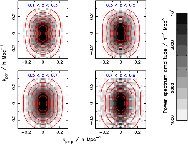
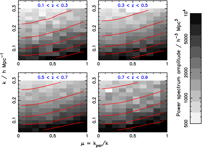
Figures 2 and 3 respectively display two-dimensional power spectra and for each of the four redshift slices, obtained by stacking measurements across the six survey regions. For comparison we also plot in each case contours corresponding to the best-fitting non-linear empirical Lorentzian redshift-space distortion model described below. In Figure 2 the non-circular nature of the measurements and models in Fourier space encode the imprint of redshift-space distortions. The overall “squeezing” of the contours in the direction reflects the large-scale bulk flows. The apparent “pinching” of the models near the axis is due to the damping caused by the pairwise velocity dispersion discussed below in Section 3.2, the amplitude of which is seen to increase with decreasing redshift (the pinching results from the relative variation with of the numerator and denominator of Equation 10). Figure 3, which bins the clustering amplitude with the cosine of the angle to the line-of-sight , illustrates how the coherent velocity flows boost the power of radial () modes relative to tangential () modes for a given scale .
3 Modelling the redshift-space galaxy power spectrum
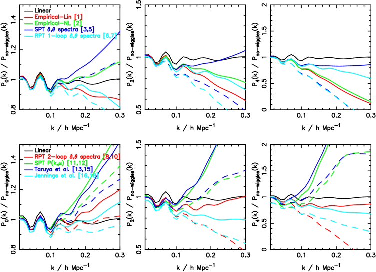
In this Section we describe a range of 18 models of the redshift-space galaxy power spectrum in the quasi-linear regime that we will try fitting to our measurements. These models are listed in Table LABEL:tabmodlist. We assume that the shape of the underlying linear matter power spectrum is accurately determined by observations of the Cosmic Microwave Background radiation, and hence we fix the background cosmological parameters. In this case each redshift-space power spectrum model contains at least two parameters to be fitted: the growth rate and a linear bias . In several cases discussed below we introduce a third parameter, a variable damping coefficient . The multipole power spectra of these models at redshift are compared in Figure 4 assuming a linear bias , a growth rate and (where applicable) a damping term km s-1. For the purposes of illustration, all models in Figure 4 are divided by a smooth “no-wiggles” reference power spectrum from the fitting formulae of Eisenstein & Hu (1998), which has the same shape as the linear power spectrum but without the imprint of baryon acoustic oscillations.
| Model | Damping | Fitted parameters | Reference | |
|---|---|---|---|---|
| 1. | Empirical Lorentzian with linear | Variable | , , | e.g. Hatton & Cole (1998) |
| 2. | Empirical Lorentzian with non-linear | Variable | , , | |
| 3. | , , from 1-loop SPT | None | , | e.g. Vishniac (1983), Juszkiewicz et al. (1984) |
| 4. | , , from 1-loop SPT | Variable | , , | |
| 5. | , , from 1-loop SPT | Linear | , | |
| 6. | , , from 1-loop RPT | None | , | Crocce & Scoccimarro (2006) |
| 7. | , , from 1-loop RPT | Linear | , | |
| 8. | , , from 2-loop RPT | None | , | |
| 9. | , , from 2-loop RPT | Variable | , | |
| 10. | , , from 2-loop RPT | Linear | , | |
| 11. | from 1-loop SPT | None | , | Matsubara (2008) |
| 12. | from 1-loop SPT | Linear | , | |
| 13. | with additional corrections | None | , | Taruya et al. (2010) |
| 14. | with additional corrections | Variable | , , | |
| 15. | with additional corrections | Linear | , | |
| 16. | Fitting formulae from N-body simulations | None | , | Smith et al. (2003), Jennings et al. (2011) |
| 17. | Fitting formulae from N-body simulations | Variable | , , | |
| 18. | Fitting formulae from N-body simulations | Linear | , |
3.1 Density and velocity power spectra
The galaxy overdensity field, , is modified in redshift-space by peculiar velocities. In Fourier space the redshift-space overdensity field is given by
| (3) |
where is the Fourier transform of the divergence of the peculiar velocity field in units of the co-moving Hubble velocity (i.e. ), , and is the cosine of the angle of the Fourier mode to the line-of-sight. Equation 3 assumes that the galaxy separation is small compared with the distance to the galaxies, and are small, the velocity field is irrotational, and the continuity equation holds. In this case the linear redshift-space power spectrum of a population of galaxies may be written
| (4) |
where , , are the isotropic galaxy-galaxy, galaxy- and - power spectra for modes , respectively. We will often refer to the as the “velocity power spectrum” although it would be better described as the “power spectrum of the velocity divergence field”.
Assuming that the velocity field is generated under linear perturbation theory then
| (5) |
where is the growth rate of structure, expressible in terms of the growth factor at cosmic scale factor as , and is the matter overdensity. The growth factor is defined in terms of the amplitude of a single perturbation as . Equation 5 additionally assumes that the linearized Euler and Poisson equations hold in a perturbed Friedmann-Robertson-Walker universe. It represents a coherent flow of matter in which there is a one-to-one coupling between the Fourier components of the velocity divergence and density fields.
Under the assumption of a deterministic, scale-independent, local, linear bias then
| (6) |
and we may write and . If we additionally assume that Equation 5 applies, then Equation 4 may be written
| (7) | |||||
Equation 7 is known as the large-scale “Kaiser limit” of the redshift-space power spectrum model (Kaiser 1987), often expressed in terms of the parameter . We assume no velocity bias between galaxies and matter (Lau, Nagai & Kravtsov 2010).
Simulations and observations have demonstrated that Equation 7 is an unreliable model on all but the largest scales (smallest values of ) due to the non-linear growth of structure. Deviations from the Kaiser limit are evident for Mpc-1 and are particularly noticeable in the power spectra (Jennings et al. 2011; Okumura et al. 2011). This failure of the model is due to the breakdown of the relation between and (Equation 5) rather than the underlying structure of Equation 4 (Scoccimarro 2004). Non-linear evolution implies that a given overdensity produces a range of values of , and this range of velocities acts to smooth the galaxy overdensity field in redshift-space, or damp the power spectra. This non-linear damping must be modelled in order to avoid introducing a systematic error into our extraction of the growth rate from data. A variety of methods are available for implementing this non-linear correction, which we discuss below.
3.2 The empirical non-linear velocity model
The standard “streaming model” for describing the non-linear component of redshift-space distortions (e.g. Hatton & Cole 1998) introduces an empirical damping function to be multiplied into Equation 4, representing convolution with uncorrelated galaxy motions on small scales:
| (8) |
The two models most commonly considered in the literature are the Lorentzian and the Gaussian , representing exponential and Gaussian convolutions in configuration space, and each parameterized by a single variable . The Lorentzian model produces better fits to data (e.g. Hawkins et al. 2003, Cabre & Gaztanaga 2009) and we assume this version of the model in our study.
Equation 8 is typically applied assuming that , and are predicted by linear theory assuming Equation 5, hence for the Lorentzian model we obtain
| (9) |
where we generated the linear power spectrum using the CAMB software package (Lewis, Challinor & Lasenby 2000). This is Model 1 in Table LABEL:tabmodlist. We also considered the case where a non-linear density power spectrum , generated by applying the fitting formula of Smith et al. (2003) to the CAMB output, is used in Equation 9:
| (10) |
This is Model 2.
Although these models are motivated by virialized motions of particles in collapsed structures, it is important to note that they are heuristic in nature. The correction represented by in fits to real data is typically of order at Mpc-1. These Fourier modes describe physical scales of tens of Mpc, far exceeding the size of virialized structures. In addition, the form of and the value of depend strongly on details such as galaxy type, dark matter halo mass and satellite fraction. However, it should be noted that Equation 9 does a very reasonable job of empirically modelling real datasets at the precision available in previous redshift surveys (e.g., Hawkins et al. 2003, Cabre & Gaztanaga 2009).
3.3 Perturbation theory approaches
A different approach to modelling clustering beyond linear scales is to extend Equations 4 and 5 into the quasi-linear regime using perturbation theory techniques. These approaches have the advantage of a stronger physical motivation compared to the empirical streaming models, and the disadvantage that they are potentially applicable for a narrower range of scales, depending on the type of perturbation expansion. Standard perturbation theory at is only accurate for the range Mpc-1, but other expansion approaches are available with the precise range of validity dependent on the model in question and the accuracy required (Nishimichi et al. 2009, Carlson et al. 2009). We describe the order of the perturbative expansion by the number of “loops” of resummation performed; calculations including up to 2 loops are currently tractable.
Various methodologies have been introduced. The simplest technique is to use perturbation theory approaches to model the quasi-linear behaviour of the functions , and in Equation 4. These techniques have been recently reviewed by Nishimichi et al. (2009) and Carlson et al. (2009) and include Eulerian standard perturbation theory (SPT; e.g. Vishniac 1983, Juszkiewicz, Sonoda & Barrow 1984) together with attempts to improve the convergence behaviour such as Renormalized Perturbation Theory (RPT; e.g. Crocce & Scoccimarro 2006) which does not expand on the amplitude of fluctuations. When generating the perturbation theory predictions we assumed an input linear power spectrum consistent with the latest CMB observations: , , , , and .†††We are very grateful to Martin Crocce for providing us with the 1-loop and 2-loop outputs of RPT for our cosmological model at the redshifts in question.
Going beyond the linear assumption may also lead to an alternative dependence of the redshift-space power spectrum on to that exhibited by Equation 4. Scoccimarro (2004) proposed the following model for the redshift-space power spectrum in terms of the quasi-linear density and velocity power spectra:
| (11) |
where is determined by
| (12) |
The power spectra , and in Equation 11 may be generated by perturbation theory or other approaches. We note that and are functions of . The damping factor in Equation 11 is analogous to the streaming model of Equation 8 but has a very different physical motivation: it aims to model the quasi-linear growth of the power spectra rather than virialized small-scale motions. Indeed, it would be possible to add an extra empirical damping factor to Equation 11 to model small-scale motions.
As discussed by Scoccimarro (2004), the model of Equation 11 is an approximation in which the Gaussian damping factor attempts to reproduce the correct non-linear behaviour; Equation 11 cannot be strictly derived from theory. Given this approximation we consider fitting as a variable parameter in addition to fixing it using Equation 12. Models 3 to 10 in Table LABEL:tabmodlist are various combinations of SPT and RPT with different implementations of the damping term.
We note that can also be expressed in velocity units by multiplying by the Hubble parameter km s-1 Mpc-1. When calculating the damping term we use the linear velocity power spectrum as the input to Equation 12; i.e. we set .
The final perturbation theory approaches we consider follow Matsubara (2008) and Taruya, Nishimichi & Saito (2010) who present quasi-linear perturbation theory models including terms up to , of the form
| (13) |
where the coefficients are functions of , which we also try fitting to our data. The Matsubara (2008) results are a full angle-dependent treatment of standard perturbation theory (Models 11 and 12), and Taruya et al. (2010) present an improved analysis incorporating additional correction terms (Models 13 to 15). When calculating the Taruya et al. model prediction we use power-spectra , and generated by 2-loop Renormalized Perturbation Theory.
3.4 Fitting formulae calibrated by simulations
Finally, N-body dark matter simulations can be exploited to calibrate the quasi-linear forms of the functions , and . The advantage of this technique is that the results will be (potentially) reliable across a wider range of scales than is accessible with perturbation theory. The disadvantage is that simulations are expensive to generate and it is difficult to span a wide range of input cosmological models (although that is not a limitation for us given that we are only considering a single fiducial model).
Smith et al. (2003) presented a widely-used prescription for generating non-linear density power spectra . Fitting formulae calibrated to N-body simulations for and as a function of redshift, in terms of , were recently proposed by Jennings et al. (2011). We inserted these fitting functions into Equation 11, scaling by and respectively to correct for the differing notation conventions. The Jennings et al. formulae, combined with various implementations of the damping term, are Models 16 to 18 in Table LABEL:tabmodlist.
4 Parameter fits
4.1 Growth rate
We fitted the 18 models introduced in Section 3 and summarized in Table LABEL:tabmodlist to the WiggleZ Survey galaxy power spectra measured in Section 2. For each of the four redshift slices we determined the growth rate fitting to the six survey regions, marginalizing over the linear bias (and the pairwise velocity dispersion where applicable). We also recorded the minimum value of the statistic for each model calculated using the full covariance matrix. We repeated this procedure varying the range of scales over which each model is fitted. Utilizing a higher value of produces an improved statistical error in the measurement, but potentially causes a larger systematic error since all models (and particularly some of the perturbation-theory models) are less reliable at larger values of for which the non-linear corrections are more significant. In the absence of systematic errors the best-fitting growth rate would be independent of .
Figure 5 displays the growth-rate measurements for the redshift slice (which produces the highest statistical accuracy of the four slices), comparing results for , and Mpc-1. At least one model can always be found that provides a good fit to the data for each of the choices of , as indicated by the minimum values of for with number of degrees of freedom . The respective probabilties for obtaining values of higher than these are , indicating an acceptable goodness-of-fit. In Figure 5 we display the minimum values of for every model relative to the best-fitting model for each choice of .
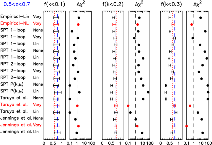
For all models provide a good fit to the data and consistent measurements of the growth rate. This confirms the convergence of the different modelling approaches at large scales. For and some models are significantly disfavoured by larger values of , and these models produce measurements of the growth rate which systematically differ from the best-performing models. For , models with a variable damping parameter produce a fit with a significantly lower value of , suggesting that Equation 12 produces an unreliable prediction of the damping coefficient for these smaller scales.
Considering all four redshift slices, the best-performing models for Mpc-1 are the Taruya et al. (2010) model, incorporating extra angle-dependent correction terms in addition to the density and velocity power spectra from 2-loop Renormalized Perturbation Theory (Model 14 in Table LABEL:tabmodlist), and the Jennings et al. (2011) fitting formula calibrated from N-body simulations (Model 17). The growth rates deduced from these two very different modelling techniques agree remarkably well, after marginalizing over the variable damping term and linear galaxy bias, with the difference in values being much smaller than the statistical errors in the measurement. The level of this agreement gives us confidence that our results are not limited by systematic errors. We note that the empirical Lorentzian streaming model, where we use the non-linear model power spectrum, also performs well (Model 2 in Table LABEL:tabmodlist). In Figure 5 we have highlighted these three models in red. For all scales and redshifts these models typically produce mutually consistent measurements of the growth rate and minimum values of which differ by . As a further comparison, Figure 6 illustrates the measurements for all 18 models in every redshift slice for , again highlighting the same three optimal models in red.
We can use the dispersion in the results of fitting these three models to estimate the systematic error in the growth rate measurement, by taking the variance of the different growth rates weighting by . The systematic error in calculated in this manner is in the four redshift slices (for Mpc-1). The magnitude of this error is less than half that of the statistical error in each bin. This systematic error represents the dispersion of growth rate determinations within the set of redshift-space distortion models listed in Table LABEL:tabmodlist.
We quote our final results using the Jennings et al. (2011) model, which usually produces the lowest value of , applied to Mpc-1. The growth rate measurements in the four redshift slices using this model, marginalizing over the other parameters, are . The values of the galaxy bias parameter in each redshift slice using this model, marginalizing over the other parameters, are .
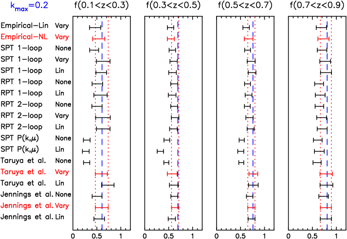
Figure 7 explores in more detail the robustness of the growth rate measurements as a function of for the three optimal models. We plot the growth rate determined in four redshift slices for these models alone, considering a range of fitting limits between and Mpc-1. Figure 7 empirically demonstrates that systematic trends in the growth rate measurement as changes are typically less than the statistical error in the measurement for .
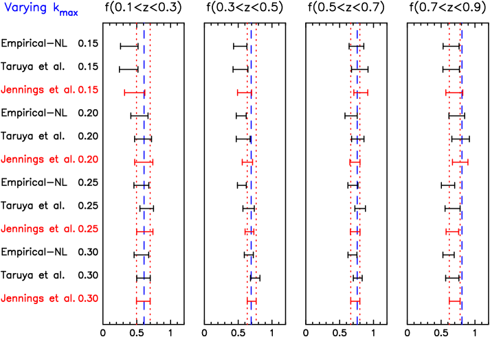
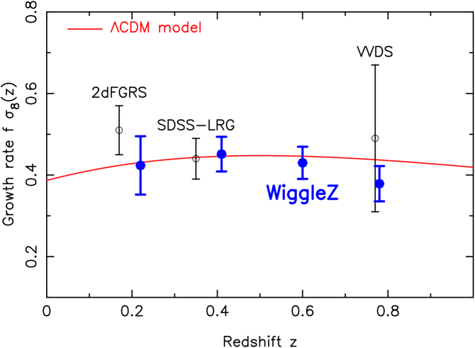
Figure 8 displays the WiggleZ Survey measurements of the growth rate of structure in four redshift slices, using the Jennings et al. (2011) model with a variable damping parameter and fitting to Mpc-1. We present our results multiplied by a redshift-dependent normalization, , where is the r.m.s. fluctuation at redshift of the linear matter density field in co-moving Mpc spheres, calculated for our fiducial cosmological model. This weighting increases the model-independence of the results by removing the sensitivity to the overall normalization of the power spectrum model (Song & Percival 2009). Because the overall galaxy power spectrum amplitude scales with at a particular redshift , where is the linear bias factor, and the magnitude of the redshift-space distortion due to coherent flows depends on , then the measured value of growth rate scales as . The weighted fits in the four redshift slices are . The WiggleZ measurements are compared to results previously published for the 2dFGRS, SDSS-LRG and VVDS samples, as collected by Song & Percival (2009), and to the prediction of a flat CDM cosmological model with . We note that:
-
•
The WiggleZ Survey dataset is the first to produce precise growth-rate measurements in the intermediate-redshift range , the apparent transition epoch from decelerating to accelerating expansion, with measurement errors that are comparable to those obtained at lower redshift from existing surveys.
-
•
The low-redshift WiggleZ measurements agree well with existing data.
-
•
Our dataset permits coherent flows to be quantified across the entire redshift range using observations from a single galaxy survey.
-
•
A cosmological model in which General Relativity describes the large-scale gravitation of the Universe, and the current matter density parameter is , provides a good simultaneous description of the initial conditions described by CMB observations, the cosmic expansion history mapped by high-redshift supernovae and baryon acoustic oscillations, and the growth history mapped by galaxy bulk flows in the WiggleZ Dark Energy Survey.
4.2 Galaxy-mass cross-correlation
In order to characterize the galaxy bias relation in more detail we introduced a cross-correlation parameter between the galaxy and matter overdensities such that and (where is required by the definition of a cross-correlation coefficient). The value corresponds to a fully deterministic bias, whereas introduces a random stochastic element to the bias relation. Measurements of this stochasticity in the SDSS were presented by Swanson et al. (2008), who utilized a counts-in-cells analysis to quantify its dependence on scale, luminosity and colour. Swanson et al. found that a scale-independent deterministic linear bias was in general a good match to the SDSS data, especially on large scales, where the amplitude of the bias varied significantly with luminosity for red galaxies but not blue galaxies. Furthermore, colour-dependent stochastic effects were evident at smaller scales. We can extend this analysis to higher redshifts using the WiggleZ power spectrum.
Equation 4 may be re-written for a general cross-correlation parameter as
| (14) |
and assuming a model for the three power spectra , and , the value of may be extracted for each scale by marginalizing over . In this investigation we fix the value of the growth rate at the value predicted by the CDM model, and we assume the Smith et al. (2003) and Jennings et al. (2011) prescriptions for the density and velocity power spectra. We also marginalized over a variable damping parameter.
Figure 9 displays the measurement of in independent Fourier bins of width Mpc-1 between and Mpc-1, combining the results for different redshift slices and varying within the range . We find that the cross-correlation parameter is consistent with deterministic bias (and this result also applies for each separate redshift slice). Because the probability distribution for is asymmetric due to the hard upper limit, in the cases when the confidence region is truncated at we plot in Figure 9 the range below enclosing of the probability, and the position of the peak of the likelihood.

5 Analysis of the power spectrum moments
5.1 Multipole moments of the power spectrum
In this Section we explore some alternative techniques for quantifying the redshift-space power spectra which can visualize their information content more neatly. The galaxy power spectrum may be decomposed in a basis of Legendre polynomials to give multipole moments :
| (15) | |||||
| (16) |
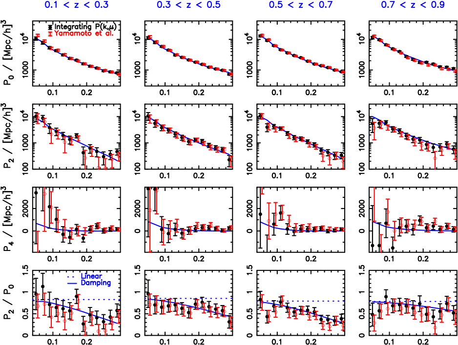
The monopole () spectrum primarily contains information about the underlying shape of the isotropic clustering pattern. The quadrupole () spectrum holds the leading-order signal from the anisotropic modulation in power due to redshift-space effects. We note that the multipole moments may be expressed in terms of the density-velocity power spectra , and (e.g. Percival & White 2009).
The multipole moments may be extracted from the power spectrum measurement in bins of by turning Equation 16 from an integral into a sum:
| (17) |
Alternatively, Yamamoto et al. (2006) introduced a direct estimator for which does not require binning of the power spectrum in (which is particularly problematic at low , where there are limited modes available in Fourier space). We present the key equations of the estimator here, referring the reader to Yamamoto et al. (2006) for the full derivation.
The Yamamoto et al. estimator, which is valid when the distant-observer approximation is applicable, is written using sums over observed galaxies and random (mock) galaxies (where ). For each Fourier mode we define the multipole moments based on the data as
| (18) |
where is the position vector of galaxy and is a weight factor for each galaxy, specified below. If we define the equivalent sum over the set of random galaxies, then an estimator for is
| (19) | |||||
where the shot noise term is given by
| (20) |
The normalization is given, in terms of sums over the grid cells constituting the window function, as
| (21) |
where is the window function normalized over its volume such that , or . The minimum variance in is produced by the usual FKP weight function
| (22) |
where is a characteristic power spectrum amplitude (which we take as Mpc3, although this choice has very little effect on our results). The error in the estimator for each Fourier mode is given by
| (23) | |||||
We evaluated the estimator for over the usual grid of Fourier modes which describe fluctuations in a cuboid of dimensions , i.e. for modes for integers . We then averaged the amplitudes in spherical shells of to produce our estimate of , which we write as . We note that the discreteness of the Fourier modes in the grid produces a bias in the estimate, which is particularly evident at low . We corrected for this bias using a model power spectrum by evaluating
| (24) | |||||
which we averaged in spherical shells of to produce , and also an exact determination using
| (25) |
Our final estimate for the multipole power spectrum is then given by
| (26) |
We generated this correction using the best-fitting non-linear empirical Lorentzian redshift-space power spectrum (see Section 3.2) as the input model .
Figure 10 compares the measurement of the multipole power spectra in four redshift slices obtained by the direct sum of Equation 17 with the Yamamoto et al. estimator of Equation 19. In general the two different techniques for deriving the multipole power spectra agree well and we obtain measurements of the monopole () and quadrupole () with high signal-to-noise. Current galaxy redshift surveys do not yield a significant detection of the hexadecapole ().
The final row of Figure 10 plots the measured quadrupole-to-monopole ratio as a function of scale for each redshift slice. This statistic has the advantage of being less sensitive than the power spectrum itself to the parameters which model the shape of the underlying real-space galaxy clustering pattern (such as the background cosmological parameters or a scale-dependent bias). On large scales this ratio is expected to asymptote to a constant value which may be derived from Equation 7:
| (27) |
where . This value, indicated by the dotted “Linear” horizontal line in the bottom row of Figure 10, and derived using the prediction of in a CDM model with , lies in good agreement with the measurements on large scales in each redshift slice. At smaller scales the data deviates from this prediction due to the non-linear effects which damp the velocity power spectrum. We also plot the scale-dependent value of for the best-fitting non-linear empirical Lorentzian redshift-space distortion model in each redshift slice, indicated by the “Damping” line.
5.2 Power spectra of the velocity divergence field
The characteristic angular dependence of the redshift-space galaxy power spectrum on its three component power spectra , and , exhibited by Equation 4, gives us the opportunity to extract these three power spectra directly from data. This is of particular interest for the case of because this quantity depends on the growth rate but not on the galaxy bias, which is considered to be one of the principle sources of potential systematic error in redshift-space distortion model-fitting.
The signal-to-noise ratio of the power spectrum measurements from current surveys is not yet sufficiently high to extract three independent functions cleanly (e.g., Tegmark et al. 2004) – which is consistent with our failure to detect the hexadecapole in Figure 10. However, a good approximation of the galaxy-velocity cross-power spectrum in the quasi-linear regime is (Percival & White 2009), which cancels (to first order) non-linear terms in the power spectra and galaxy bias. Under this approximation we can fit for the coefficients and in the model (Song & Kayo 2010)
| (28) |
For each separate -bin, spaced by Mpc-1, we fitted the model of Equation 28 to the stacked measurements of from the WiggleZ survey dataset in four redshift slices. We performed the fit in 10 Fourier bins up to Mpc-1, choosing this upper limit because Equation 4 will likely not provide a reliable description of the -dependence of the power spectrum at smaller scales (given that our model fits in Section 4.1 favour the inclusion of an additional Lorentzian damping term over the range Mpc-1).
Figure 11 displays the results of the fits for each redshift slice, where for convenience we have divided the measurements of by the best-fitting value of so that the galaxy and velocity power spectra are expected to have the same large-scale limit. For comparison we also plot in each case the non-linear galaxy and velocity power spectra based on the fitting formulae proposed by Smith et al. (2003) and Jennings et al. (2011), respectively, together with the underlying linear matter power spectrum for our fiducial cosmological parameters at these redshifts.
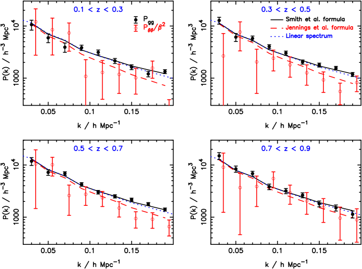
Our measurements constitute the first determination of the velocity power spectrum as a function of redshift, and cleanly reveal the effects that we are modelling. At large scales Mpc-1 the density and velocity power spectra are in close agreement with each other and the input model linear power spectrum. At smaller scales the measurements diverge: the density power spectra are boosted in amplitude in a manner that closely matches the fitting formula of Smith et al. (2003), and the velocity power spectra are damped by non-linear effects. The fitting formula of Jennings et al. (2011) provides a good match to this damping: the value of statistic is for the four redshift slices respectively, for 10 degrees of freedom. The value of for the highest redshift bin corresponds to a 2- fluctuation. As the values for the other three redshift slices fall within the 1- range for the distribution, we do not view this with concern. We also find a tentative indication that the amplitude of the non-linear correction to the velocity power spectrum increases with decreasing redshift, expected as a consequence of the growth of structure.
6 Conclusions
We have used the WiggleZ Dark Energy Survey dataset to produce the first precise map of cosmic growth spanning the epoch of cosmic acceleration and the first systematic study of the growth history from a single galaxy survey. We have compared the measured power spectra to 18 different redshift-space distortion models using a combination of empirical models, fitting formulae calibrated by N-body simulations, and perturbation theory techniques. We itemize our conclusions as follows:
-
•
Two quasi-linear redshift-space distortion models provide a good description of our data for scales Mpc-1: the Taruya et al. (2010) model, incorporating extra angle-dependent correction terms in addition to the density and velocity power spectra from 2-loop Renormalized Perturbation Theory, and the Jennings et al. (2011) fitting formula calibrated from N-body simulations. In each model we included a variable damping parameter. The growth rates deduced from these two very different modelling techniques agree remarkably well, with the difference in values being much smaller than the statistical errors in the measurement. The level of this agreement gives us confidence that our results are not limited by systematic errors. We note that the empirical Lorentzian streaming model, where we use the non-linear matter power spectrum from Smith et al. (2003), also performs well and the minimum chi-squared values for these three models typically differ by . We quote our final results using the Jennings et al. (2011) model, which usually produces the lowest value of : growth rate measurements of at redshifts , where we have marginalized over the variable damping factor and a linear galaxy bias factor. A more model-independent way of expressing these fits is .
-
•
These growth rate measurements are consistent with those expected in a flat General Relativistic CDM cosmological model with matter density . Our observations therefore indicate that this model provides a self-consistent description of the growth of cosmic structure from perturbations and the large-scale, homogeneous cosmic expansion mapped by supernovae and baryon acoustic oscillations.
-
•
Assuming the growth rate predicted by the CDM model we can fit for the parameters of a stochastic scale-dependent bias described by a galaxy-mass cross-correlation . We find that this bias is consistent with a deterministic model for the range of scales Mpc-1.
-
•
We considered various methods for presenting the information contained in the redshift-space power spectra, including deriving the multipole moments using direct integration of the binned power spectrum and by implementing the estimator described by Yamamoto et al. (2006). Measurements of the quadrupole-to-monopole ratio as a function of scale delineate the influence of redshift space distortions in a manner independent of the shape of the underlying matter power spectrum or a scale-dependent bias.
-
•
Under the assumption , which is a good approximation in the quasi-linear regime, we used the redshift-space power spectra to fit directly for and . We found that (within an overall normalization factor) the galaxy and velocity power spectra are consistent with each other and with the model linear power spectrum at low . For Mpc-1 we delineated for the first time the characteristic non-linear damping of the velocity power spectrum as a function of redshift, with a tentative indication that the amplitude of the non-linear effects increases with decreasing redshifts. The Jennings et al. (2011) fitting formula provides a good fit to these power spectra.
A future investigation will involve the confrontation of this data with a range of modified-gravity models, combining the large-scale structure measurements with self-consistent fits to the Cosmic Microwave Background observations. Furthermore, a joint analysis of the redshift-space distortions and Alcock-Paczynski effect is also in preparation.
Acknowledgments
We thank Carlton Baugh, Elise Jennings, Juliana Kwan, David Parkinson, Will Percival, Roman Scoccimarro and Yong-Seon Song for useful comments which influenced and improved the development of this paper. We are particularly grateful to Martin Crocce for providing power spectra for Renormalized Perturbation Theory and for helpful comments.
We acknowledge financial support from the Australian Research Council through Discovery Project grants funding the positions of SB, MP, GP and TD. SMC acknowledges the support of the Australian Research Council through a QEII Fellowship. MJD and TD thank the Gregg Thompson Dark Energy Travel Fund for financial support.
GALEX (the Galaxy Evolution Explorer) is a NASA Small Explorer, launched in April 2003. We gratefully acknowledge NASA’s support for construction, operation and science analysis for the GALEX mission, developed in co-operation with the Centre National d’Etudes Spatiales of France and the Korean Ministry of Science and Technology.
Finally, the WiggleZ survey would not be possible without the dedicated work of the staff of the Australian Astronomical Observatory in the development and support of the AAOmega spectrograph, and the running of the AAT.
References
- [1] da Angela J., et al., 2008, MNRAS, 383, 565
- [2] Blake C.A., et al., 2009, MNRAS, 395, 240
- [3] Blake C.A., et al., 2010, MNRAS, 406, 803
- [4] Cabre A., Gaztanaga E., 2009, MNRAS, 393, 1183
- [5] Carlson J., White M., Padmanabhan N., 2010, Phys. Rev. D80, 3531
- [6] Cole S., Kaiser N., 1989, MNRAS, 237, 1127
- [7] Crocce M., Scoccimarro R., 2006, Phys. Rev. D73, 63519
- [8] Davis T.M., et al., 2007, ApJ, 666, 716
- [9] Dekel A., Lahav O., 1999, ApJ, 520, 24
- [10] Drinkwater M., et al., 2010, MNRAS, 401, 1429
- [11] Eisenstein D.J., Hu W., 1998, ApJ, 496, 605
- [12] Feldman H.A., Kaiser N., Peacock J.A., 1994, ApJ, 426, 23
- [13] Gilbank D.G., Gladders M.G., Yee H.K.C., Hsieh B.C., 2011, AJ, 141, 94
- [14] Guy J., et al., 2010, A&A, 523, 7
- [15] Guzzo L., et al., 2008, Nature, 451, 541
- [16] Hamilton A.J.S., 1998, “Linear redshift distortions: A review”, in “The Evolving Universe”, ed. D.Hamilton, pp.185-275 (Kluwer Academic, 1998) [astro-ph/9708102]
- [17] Hatton S., Cole S., 1998, MNRAS, 296, 10
- [18] Hawkins E., et al., 2003, MNRAS, 346, 78
- [19] Jennings E., Baugh C.M., Pascoli S., 2011, MNRAS, 410, 2081
- [20] Jing Y., 2005, ApJ, 620, 559
- [21] Juszkiewicz R., Sonoda D.H., Barrow J.D., 1984, MNRAS, 209, 139
- [22] Kaiser N., 1987, MNRAS, 227, 1
- [23] Komatsu E., et al., 2009, ApJS, 180, 330
- [24] Lau E.T., Nagai D., Kravtsov A.V., 2010, ApJ, 708, 1419
- [25] Lewis A., Challinor A., Lasenby A., 2000, ApJ, 538, 473
- [26] Linder E., Jenkins A., 2003, MNRAS, 346, 573
- [27] Linder E., 2005, Phys. Rev. D72, 3529
- [28] Linder E., Cahn R., 2007, APh, 28, 481
- [29] Matsubara T., 2008, Phys. Rev. D77, 063530
- [30] Nesseris S., Perivolaropoulos L., 2008, Phys. Rev. D77, 023504
- [31] Nishimichi T., et al., 2009, PASJ, 61, 321
- [32] Okumura T., Matsubara T., Eisenstein D.J., Kayo I., Hikage C., Szalay A.S., Schneider D.P., 2008, ApJ, 676, 889
- [33] Okumura T., Jing Y.P., 2011, ApJ, 726, 5
- [34] Peacock J.A., et al., 2001, Nature, 410, 169
- [35] Percival W.J., et al., 2004, MNRAS, 353, 1201
- [36] Percival W.J., White M., 2009, MNRAS, 393, 297
- [37] Percival W.J., et al., 2010, MNRAS, 401, 2148
- [38] Raccanelli A., Samushia L., Percival W.J., 2010, MNRAS, 409, 1525
- [39] Reid B.A., et al., 2010, MNRAS, 404, 60
- [40] Rimes C.D., Hamilton A.J.S., 2005, MNRAS, 360, 82
- [41] Rubin D., et al., 2009, ApJ, 695, 391
- [42] Scoccimarro R., 2004, Phys. Rev. D70, 083007
- [43] Scherrer R.J., Weinberg D.H., 1998, ApJ, 504, 607
- [44] Sharp R. et al., 2006, SPIE, 6269E, 14
- [45] Smith R.E., et al., 2003, MNRAS, 341, 1311
- [46] Song Y.-S., Percival W.J., 2009, JCAP, 10, 4
- [47] Song Y.-S., Kayo, 2010, MNRAS, 407, 1123
- [48] Swanson M.E.C., Tegmark M., Blanton M., Zehavi I., 2008, MNRAS, 385, 1635
- [49] Takahashi R., et al., 2011, ApJ, 726, 7
- [50] Taruya A., Nishimichi T., Saito S., 2010, Phys. Rev. D82, 3522
- [51] Tegmark M., et al., 2004, ApJ, 606, 702
- [52] Tegmark M., et al., 2006, Phys. Rev. D74, 123507
- [53] Vishniac E.T., 1983, MNRAS, 203, 345
- [54] Wang Y., 2008, JCAP, 5, 21
- [55] Wiltshire D.L., 2009, Phys. Rev. D80 123512
- [56] Yamamoto K., Nakamichi M., Kamino A., Bassett B.A., Nishioka H., 2006, PASJ, 58, 93