Cluster Forests

Abstract

With inspiration from Random Forests (RF) in the context of classification, a new clustering ensemble method—Cluster Forests (CF) is proposed. Geometrically, CF randomly probes a high-dimensional data cloud to obtain “good local clusterings” and then aggregates via spectral clustering to obtain cluster assignments for the whole dataset. The search for good local clusterings is guided by a cluster quality measure kappa. CF progressively improves each local clustering in a fashion that resembles the tree growth in RF. Empirical studies on several real-world datasets under two different performance metrics show that CF compares favorably to its competitors. Theoretical analysis reveals that the kappa measure makes it possible to grow the local clustering in a desirable way—it is “noise-resistant”. A closed-form expression is obtained for the mis-clustering rate of spectral clustering under a perturbation model, which yields new insights into some aspects of spectral clustering.

1 Motivation

The general goal of clustering is to partition a set of data such that data points within the same cluster are “similar” while those from different clusters are “dissimilar.” An emerging trend is that new applications tend to generate data in very high dimensions for which traditional methodologies of cluster analysis do not work well. Remedies include dimension reduction and feature transformation, but it is a challenge to develop effective instantiations of these remedies in the high-dimensional clustering setting. In particular, for datasets whose dimension is beyond $20$, it is infeasible to perform full subset selection. Also, there may not be a single set of attributes on which the whole set of data can be reasonably separated. Instead, there may be local patterns in which different choices of attributes or different projections reveal the clustering.

Our approach to meeting these challenges is to randomly probe the data/feature space to detect many locally “good” clusterings and then aggregate by spectral clustering. The intuition is that, in high-dimensional spaces, there may be projections or subsets of the data that are well separated and these projections or subsets may carry information about the cluster membership of the data involved. If we can effectively combine such information from many different views (here a view has two components, the directions or projections we are looking at and the part of data that are involved), then we can hope to recover the cluster assignments for the whole dataset. However, the number of projections or subsets that are potentially useful tend to be huge, and it is not feasible to conduct a grand tour of the whole data space by exhaustive search. This motivates us to randomly probe the data space and then aggregate.

The idea of random projection has been explored in various problem domains such as clustering [9, 12], manifold learning [20] and compressive sensing [10]. However, the most direct motivation for our work is the Random Forests (RF) methodology for classification [7]. In RF, a bootstrap step selects a subset of data while the tree growth step progressively improves a tree from the root downwards—each tree starts from a random collection of variables at the root and then becomes stronger and stronger as more nodes are split. Similarly, we expect that it will be useful in the context of high-dimensional clustering to go beyond simple random probings of the data space and to perform a controlled probing in hope that most of the probings are “strong.” This is achieved by progressively refining our “probings” so that eventually each of them can produce relatively high-quality clusters although they may start weak. In addition to the motivation from RF, we note that similar ideas have been explored in the projection pursuit literature for regression analysis and density estimation (see [23] and references therein).

RF is a supervised learning methodology and as such there is a clear goal to achieve, i.e., good classification or regression performance. In clustering, the goal is less apparent. But significant progress has been made in recent years in treating clustering as an optimization problem under an explicitly defined cost criterion; most notably in the spectral clustering methodology [41, 44]. Using such criteria makes it possible to develop an analog of RF in the clustering domain.

Our contributions can be summarized as follows. We propose a new cluster ensemble method that incorporates model selection and regularization. Empirically CF compares favorably to some popular cluster ensemble methods as well as spectral clustering. The improvement of CF over the base clustering algorithm ($K$-means clustering in our current implementation) is substantial. We also provide some theoretical support for our work: (1) Under a simplified model, CF is shown to grow the clustering instances in a “noise-resistant” manner; (2) we obtain a closed-form formula for the mis-clustering rate of spectral clustering under a perturbation model that yields new insights into aspects of spectral clustering that are relevant to CF.

The remainder of the paper is organized as follows. In Section 2, we present a detailed description of CF. Related work is discussed in Section 3. This is followed by an analysis of the $\kappa$ criterion and the mis-clustering rate of spectral clustering under a perturbation model in Section 4. We evaluate our method in Section 5 by simulations on Gaussian mixtures and comparison to several popular cluster ensemble methods as well as spectral clustering on some UC Irvine machine learning benchmark datasets. Finally we conclude in Section 6.

2 The Method

CF is an instance of the general class of cluster ensemble methods [38], and as such it is comprised of two phases: one which creates many cluster instances and one which aggregates these instances into an overall clustering. We begin by discussing the cluster creation phase.

2.1 Growth of clustering vectors

CF works by aggregating many instances of clustering problems, with each instance based on a different subset of features (with varying weights). We define the feature space $\mathcal{F}=\{1,2,\ldots,p\}$ as the set of indices of coordinates in $\mathbb{R}^{p}$. We assume that we are given $n$ i.i.d. observations $X_{1},\ldots,X_{n}\in\mathbb{R}^{p}$. A clustering vector is defined to be a subset of the feature space.

Definition 1. The growth of a clustering vector is governed by the following cluster quality measure:

$$\kappa(\bm{\tilde{f}})=\frac{SS_{W}(\bm{\tilde{f}})}{SS_{B}(\bm{\tilde{f}})},$$ (1)

where $SS_{W}$ and $SS_{B}$ are the within-cluster and between-cluster sum of squared distances (see Section 7.2), computed on the set of features currently in use (denoted by $\bm{\tilde{f}}$), respectively.

Using the quality measure $\kappa$, we iteratively expand the clustering vector. Specifically, letting $\tau$ denote the number of consecutive unsuccessful attempts in expanding the clustering vector $\bm{\tilde{f}}$, and letting $\tau_{m}$ be the maximal allowed value of $\tau$, the growth of a clustering vector is described in Algorithm 1.

Algorithm 1  The growth of a clustering vector $\bm{\tilde{f}}$

1:  Initialize $\bm{\tilde{f}}$ to be NULL and set $\tau=0$;

2:  Apply feature competition and update $\bm{\tilde{f}}\leftarrow(f_{1}^{(0)},\ldots,f_{b}^{(0)})$;

3:  repeat

4:     Sample $b$ features, denoted as $f_{1},\ldots,f_{b}$, from the feature space $\mathcal{F}$;

5:     Apply $K$-means (the base clustering algorithm) to the data induced by the feature vector $(\bm{\tilde{f}},f_{1},\ldots,f_{b})$;

6:     if $\kappa(\bm{\tilde{f}},f_{1}\ldots,f_{b})<\kappa(\bm{\tilde{f}})$ then

7:        expand $\bm{\tilde{f}}$ by $\bm{\tilde{f}}\leftarrow(\bm{\tilde{f}},f_{1},\ldots,f_{b})$ and set $\tau\leftarrow 0$;

8:     else

9:        discard $\{f_{1},\ldots,f_{b}\}$ and set $\tau\leftarrow\tau+1$;

10:     end if

11:  until $\tau\geq\tau_{m}$.

Algorithm 2  Feature competition

1:  for $i=1$ $\bf{to}$ $q$ do

2:     Sample $b$ features, $f_{1}^{(i)},\ldots,f_{b}^{(i)}$, from the feature space $\mathcal{F}$;

3:     Apply $K$-means to the data projected on $(f_{1}^{(i)},\ldots,f_{b}^{(i)})$ to get $\kappa(f_{1}^{(i)},\ldots,f_{b}^{(i)})$;

4:  end for

5:  Set $(f_{1}^{(0)},\ldots,f_{b}^{(0)})\leftarrow\arg\min_{i=1}^{q}\kappa(f_{1}^{(i)},\ldots,f_{b}^{(i)})$.

Step 2 in Algorithm 1 is called feature competition (setting $q=1$ reduces to the usual mode). It aims to provide a good initialization for the growth of a clustering vector. The feature competition procedure is detailed in Algorithm 2.

Feature competition is motivated by Theorem 1 in Section 4.1—it helps prevent noisy or “weak” features from entering the clustering vector at the initialization, and, by Theorem 1, the resulting clustering vector will be formed by “strong” features which can lead to a “good” clustering instance. This will be especially helpful when the number of noisy or very weak features is large. Note that feature competition can also be applied in other steps in growing the clustering vector. A heuristic for choosing $q$ is based on the “feature profile plot,” a detailed discussion of which is provided in Section 5.2.

2.2 The CF algorithm

The CF algorithm is detailed in Algorithm 3. The key steps are: (a) grow $T$ clustering vectors and obtain the corresponding clusterings; (b) average the clustering matrices to yield an aggregate matrix $P$; (c) regularize $P$; and (d) perform spectral clustering on the regularized matrix. The regularization step is done by thresholding $P$ at level $\beta_{2}$; that is, setting $P_{ij}$ to be $0$ if it is less than a constant $\beta_{2}\in(0,1)$, followed by a further nonlinear transformation $P\leftarrow\exp(\beta_{1}P)$ which we call scaling.

Algorithm 3  The CF algorithm

1:  for $l=1$ $\bf{to}$ $T$ do

2:     Grow a clustering vector, $\bm{\tilde{f}}^{(l)}$, according to Algorithm 1;

3:     Apply the base clustering algorithm to the data induced by clustering vector $\bm{\tilde{f}}^{(l)}$ to get a partition of the data;

4:     Construct $n\times n$ co-cluster indicator matrix (or affinity matrix) $P^{(l)}$

$$P_{ij}^{(l)}=\left\{\begin{array}[]{ll}1,&~{}\mbox{if}~{}X_{i}~{}\mbox{and}~{}X_{j}~{}\mbox{are in the same cluster}\\ 0,&~{}\mbox{otherwise};\end{array}\right.$$

5:  end for

6:  Average the indicator matrices to get $P\leftarrow\frac{1}{T}\sum_{l=1}^{T}P^{(l)}$;

7:  Regularize the matrix $P$;

8:  Apply spectral clustering to $P$ to get the final clustering.

We provide some justification for our choice of spectral clustering in Section 4.2. As the entries of matrix $P$ can be viewed as encoding the pairwise similarities between data points (each $P^{(l)}$ is a positive semidefinite matrix and the average matrix $P$ is thus positive semidefinite and a valid kernel matrix), any clustering algorithm based on pairwise similarity can be used as the aggregation engine. Throughout this paper, we use normalized cuts (Ncut, [36]) for spectral clustering.

3 Related Work

In this section, we compare and contrast CF to other work on cluster ensembles. It is beyond our scope to attempt a comprehensive review of the enormous body of work on clustering, please refer to [24, 19] for overview and references. We will also omit a discussion on classifier ensembles, see [19] for references. Our focus will be on cluster ensembles. We discuss the two phases of cluster ensembles, namely, the generation of multiple clustering instances and their aggregation, separately.

For the generation of clustering instances, there are two main approaches—data re-sampling and random projection. [11] and [30] produce clustering instances on bootstrap samples from the original data. Random projection is used by [12] where each clustering instance is generated by randomly projecting the data to a lower-dimensional subspace. These methods are myopic in that they do not attempt to use the quality of the resulting clusterings to choose samples or projections. Moreover, in the case of random projections, the choice of the dimension of the subspace is myopic. In contrast, CF proceeds by selecting features that progressively improve the quality (measured by $\kappa$) of individual clustering instances in a fashion resembling that of RF. As individual clustering instances are refined, better final clustering performance can be expected. We view this non-myopic approach to generating clustering instances as essential when the data lie in a high-dimensional ambient space. Another possible approach is to generate clustering instances via random restarts of a base clustering algorithm such as $K$-means [14].

The main approaches to aggregation of clustering instances are the co-association method [38, 15] and the hyper-graph method [38]. The co-association method counts the number of times two points fall in the same cluster in the ensemble. The hyper-graph method solves a $k$-way minimal cut hyper-graph partitioning problem where a vertex corresponds to a data point and a link is added between two vertices each time the two points meet in the same cluster. Another approach is due to [39], who propose to combine clustering instances with mixture modeling where the final clustering is identified as a maximum likelihood solution. CF is based on co-association, specifically using spectral clustering for aggregation. Additionally, CF incorporates regularization such that the pairwise similarity entries that are close to zero are thresholded to zero. This yields improved clusterings as demonstrated by our empirical studies.

A different but closely related problem is clustering aggregation [17] which requires finding a clustering that “agrees” as much as possible with a given set of input clustering instances. Here these clustering instances are assumed to be known and the problem can be viewed as the second stage of clustering ensemble. Also related is ensemble selection [8, 13, 5] which is applicable to CF but this is not the focus of the present work. Finally there is unsupervised learning with random forests [7, 37] where RF is used for deriving a suitable distance metric (by synthesizing a copy of the data via randomization and using it as the “contrast” pattern); this methodology is fundamentally different from ours.

4 Theoretical Analysis

In this section, we provide a theoretical analysis of some aspects of CF. In particular we develop theory for the $\kappa$ criterion, presenting conditions under which CF is “noise-resistant.” By “noise-resistant” we mean that the algorithm can prevent a pure noise feature from entering the clustering vector. We also present a perturbation analysis of spectral clustering, deriving a closed-form expression for the mis-clustering rate.

4.1 CF with $\kappa$ is noise-resistant

We analyze the case in which the clusters are generated by a Gaussian mixture:

$$\Delta\mathcal{N}(\bm{\mu},\Sigma)+(1-\Delta)\mathcal{N}(-\bm{\mu},\Sigma),$$ (2)

where $\Delta\in\{0,1\}$ with $\mathbb{P}(\Delta=1)=\pi$ specifies the cluster membership of an observation, and $\mathcal{N}(\bm{\mu},\Sigma)$ stands for a Gaussian random variable with mean $\bm{\mu}=(\mu[1],\ldots,\mu[p])\in\mathbb{R}^{p}$ and covariance matrix $\Sigma$. We specifically consider $\pi=\frac{1}{2}$ and $\Sigma=\bm{I}_{p\times p}$; this is a simple case which yields some insight into the feature selection ability of CF. We start with a few definitions.

Definition 2. Let $h:\mathbb{R}^{p}\mapsto\{0,1\}$ be a decision rule. Let $\Delta$ be the cluster membership for observation $X$. A loss function associated with $h$ is defined as

$$l(h(X),\Delta)=\left\{\begin{array}[]{cl}0,&~{}\mbox{if}~{}h(X)=\Delta\\ 1,&~{}\mbox{otherwise}.\end{array}\right.$$ (3)

The optimal clustering rule under (3) is defined as

$$h^{*}=\arg\min_{h\in\mathcal{G}}\mathbb{E}l(h(X),\Delta),$$ (4)

where $\mathcal{G}\triangleq\left\{h:~{}\mathbb{R}^{p}\mapsto\{0,1\}\right\}$ and the expectation is taken with respect to the random vector $(X,\Delta)$.

Definition 3 [34]. For a probability measure $Q$ on $\mathbb{R}^{d}$ and a finite set $A\subseteq\mathbb{R}^{d}$, define the within cluster sum of distances by

$$\Phi(A,Q)=\int\min_{a\in A}\phi(||x-a||)Q(dx),$$ (5)

where $\phi(||x-a||)$ defines the distance between points $x$ and $a\in A$. $K$-means clustering seeks to minimize $\Phi(A,Q)$ over a set $A$ with at most $K$ elements. We focus on the case $\phi(x)=x^{2}$, $K=2$ and refer to

$$\{\mu_{0}^{*},\mu_{1}^{*}\}=\arg\min_{A}~{}\Phi(A,Q)$$

as the population cluster centers.

Definition 4. The $i^{th}$ feature is called a noise feature if $\mu[i]=0$ where $\mu[i]$ denotes the $i^{th}$ coordinate of $\bm{\mu}$. A feature is “strong” (“weak”) if $|\mu[i]|$ is “large” (“small”).

Theorem 1.

Assume the cluster is generated by Gaussian mixture (2) with $\Sigma=\bm{I}$ and $\pi=\frac{1}{2}$. Assume one feature is considered at each step and duplicate features are excluded. Let $\mathcal{I}\neq\emptyset$ be the set of features currently in the clustering vector and let $f_{n}$ be a noise feature such that $f_{n}\notin\mathcal{I}$. If $\sum_{i\in\mathcal{I}}\left(\mu_{0}^{*}[i]-\mu_{1}^{*}[i]\right)^{2}>0$, then $\kappa(\mathcal{I})<\kappa(\{\mathcal{I},f_{n}\})$.

Remark. The interpretation of Theorem 1 is that noise features are generally not included in cluster vectors under the CF procedure; thus, CF with the $\kappa$ criterion is noise-resistant.

The proof of Theorem 1 is in the appendix. It proceeds by explicitly calculating $SS_{B}$ and $SS_{W}$ (see Section 7.2) and thus an expression for $\kappa=SS_{W}/SS_{B}$. The calculation is facilitated by the equivalence, under $\pi=\frac{1}{2}$ and $\Sigma=\bm{I}$, of $K$-means clustering and the optimal clustering rule $h^{*}$ under loss function (3).

4.2 Quantifying the mis-clustering rate

Recall that spectral clustering works on a weighted similarity graph $\mathcal{G}(\bm{V},P)$ where $\bm{V}$ is formed by a set of data points, $X_{i},i=1,\ldots,n$, and $P$ encodes their pairwise similarities. Spectral clustering algorithms compute the eigendecomposition of the Laplacian matrix (often symmetrically normalized as $\mathcal{L}(P)=D^{-1/2}(I-P)D^{-1/2}$ where $D$ is a diagonal matrix with diagonals being degrees of $\mathcal{G}$). Different notions of similarity and ways of using the spectral decomposition lead to different spectral cluster algorithms [36, 28, 32, 25, 41, 44]. In particular, Ncut [36] forms a bipartition of the data according to the sign of the components of the second eigenvector (i.e., corresponding to the second smallest eigenvalue) of $\mathcal{L}(P)$. On each of the two partitions, Ncut is then applied recursively until a stopping criterion is met.

There has been relatively little theoretical work on spectral clustering; exceptions include [4, 32, 25, 40, 31, 1, 42]. Here we analyze the mis-clustering rate for symmetrically normalized spectral clustering. For simplicity we consider the case of two clusters under a perturbation model.

Assume that the similarity (affinity) matrix can be written as

$$P=\overline{P}+\varepsilon,$$ (6)

where

$$\overline{P}_{ij}=\left\{\begin{array}[]{ll}1-\nu,&~{}\mbox{if}~{}i,j\leq n_{1}~{}\text{or}~{}i,j>n_{1}\vspace{1pt}\\ \nu,&~{}\mbox{otherwise},\end{array}\right.$$

and $\varepsilon=(\varepsilon_{ij})_{1}^{n}$ is a symmetric random matrix with $\mathbb{E}\varepsilon_{ij}=0$. Here $n_{1}$ and $n_{2}$ are the size of the two clusters. Let $n_{2}=\gamma n_{1}$ and $n=n_{1}+n_{2}$. Without loss of generality, assume $\gamma\leq 1$. Similar models have been studied in earlier work; see, for instance, [21, 33, 2, 6]. Our focus is different; we aim at the mis-clustering rate due to perturbation. Such a model is appropriate for modeling the similarity (affinity) matrix produced by CF. For example, Figure 1 shows the affinity matrix produced by CF on the Soybean data [3]; this matrix is nearly block-diagonal with each block corresponding to data points from the same cluster (there are four of them in total) and the off-diagonal elements are mostly close to zero. Thus a perturbation model such as (6) is a good approximation to the similarity matrix produced by CF and can potentially allow us to gain insights into the nature of CF.

Let $\mathcal{M}$ be the mis-clustering rate, i.e., the proportion of data points assigned to a wrong cluster (i.e., $h(X)\neq\Delta$). Theorem 2 characterizes the expected value of $\mathcal{M}$ under perturbation model (6).

Theorem 2.

Assume that $\varepsilon_{ij}$, $i\geq j$ are mutually independent $\mathcal{N}(0,\sigma^{2})$. Let $0<\nu\ll\gamma\leq 1$. Then

$$\lim_{n\rightarrow\infty}\frac{1}{n}\log(\mathbb{E}\mathcal{M})=-\frac{\gamma^{2}}{2\sigma^{2}(1+\gamma)(1+\gamma^{3})}.$$ (7)

Figure 1: The affinity matrix produced by CF for the Soybean dataset with $4$ clusters. The number of clustering vectors in the ensemble is $100$.

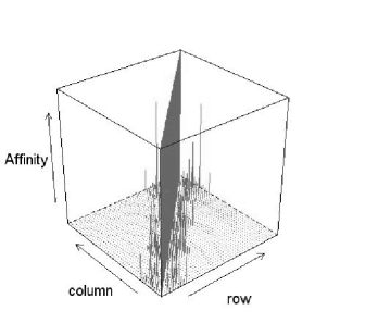
The proof is in the appendix. The main step is to obtain an analytic expression for the second eigenvector of $\mathcal{L}(P)$. Our approach is based on matrix perturbation theory [27], and the key idea is as follows.

Let $\mathfrak{P}(A)$ denote the eigenprojection of a linear operator $A:\mathbb{R}^{n}\rightarrow\mathbb{R}^{n}$. Then, $\mathfrak{P}(A)$ can be expressed explicitly as the following contour integral

$$\mathfrak{P}(A)=\frac{1}{2\pi i}\oint_{\Gamma}(A-\zeta I)^{-1}d\zeta,$$ (8)

where $\Gamma$ is a simple Jordan curve enclosing the eigenvalues of interest (i.e., the first two eigenvalues of matrix $\mathcal{L}(P)$) and excluding all others. The eigenvectors of interest can then be obtained by

$$\varphi_{i}=\mathfrak{P}\omega_{i},\quad i=1,2,$$ (9)

where $\omega_{i},i=1,2$ are fixed linearly independent vectors in $\mathbb{R}^{n}$. An explicit expression for the second eigenvector can then be obtained under perturbation model (6), which we use to calculate the final mis-clustering rate.

Remarks. While formula (7) is obtained under some simplifying assumptions, it provides insights into the nature of spectral clustering.

1. The mis-clustering rate increases as $\sigma$ increases.

2. By checking the derivative, the right-hand side of (7) can be seen to be a unimodal function of $\gamma$, minimized at $\gamma=1$ with a fixed $\sigma$. Thus the mis-clustering rate decreases as the cluster sizes become more balanced.

3. When $\gamma$ is very small, i.e., the clusters are extremely unbalanced, spectral clustering is likely to fail.

These results are consistent with existing empirical findings. In particular, they underscore the important role played by the ratio of two cluster sizes, $\gamma$, on the mis-clustering rate. Additionally, our analysis (in the proof of Theorem 2) also implies that the best cutoff value (when assigning cluster membership based on the second eigenvector) is not exactly zero but shifts slightly towards the center of those components of the second eigenvector that correspond to the smaller cluster. Related work has been presented by [22] who study an end-to-end perturbation yielding a final mis-clustering rate that is approximate in nature. Theorem 2 is based on a perturbation model for the affinity matrix and provides, for the first time, a closed-form expression for the mis-clustering rate of spectral clustering under such a model.

5 Experiments

We present results from two sets of experiments, one on synthetic data, specifically designed to demonstrate the feature selection and “noise-resistance” capability of CF, and the other on several real-world datasets [3] where we compare the overall clustering performance of CF with several competitors, as well as spectral clustering, under two different metrics. These experiments are presented in separate subsections.

5.1 Feature selection capability of CF

In this subsection, we describe three simulations that aim to study the feature selection capability and “noise-resistance” feature of CF. Assume the underlying data are generated i.i.d. by Gaussian mixture (2).

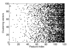
In the first simulation, a sample of $4000$ observations is generated from (2) with $\bm{\mu}=(0,\ldots,0,1,2,\ldots,100)^{T}$ and the diagonals of $\Sigma$ are all $1$ while the non-diagonals are i.i.d. uniform from $[0,0.5]$ subject to symmetry and positive definitiveness of $\Sigma$. Denote this dataset as $\bm{G}_{1}$. At each step of cluster growing one feature is sampled from $\mathcal{F}$ and tested to see if it is to be included in the clustering vector by the $\kappa$ criterion. We run the clustering vector growth procedure until all features have been attempted with duplicate features excluded. We generate $100$ clustering vectors using this procedure. In Figure 2, all but one of the $100$ clustering vectors include at least one feature from the top three features (ranked according to the $|\mu[i]|$ value) and all clustering vectors contain at least one of the top five features.

Figure 2: The occurrence of individual features in the $100$ clustering vectors for $\bm{G}_{1}$. The left plot shows the features included (indicated by a solid circle) in each clustering vector. Each horizontal line corresponds to a clustering vector. The right plot shows the total number of occurrences of each feature.

Figure 3: The occurrence of individual features in the $100$ clustering vectors for $\bm{G}_{2}$ and $\bm{G}_{3}$. The left plot is for $\bm{G}_{2}$ where the first $100$ features are noise features. The right plot is for $\bm{G}_{3}$ where the first $1000$ features are noisy features.

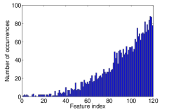
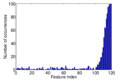
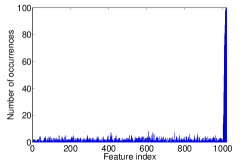
We also performed a simulation with “noisy” data. In this simulation, data are generated from (2) with $\Sigma=\bm{I}$, the identity matrix, such that the first $100$ coordinates of $\bm{\mu}$ are $0$ and the next $20$ are generated i.i.d. uniformly from $[0,1]$. We denote this dataset as $\bm{G}_{2}$. Finally, we also considered an extreme case where data are generated from (2) with $\Sigma=\bm{I}$ such that the first $1000$ features are noise features and the remaining $20$ are useful features (with coordinates of $\mu$ from $\pm 1$ to $\pm 20$); this is denoted as $\bm{G}_{3}$. The occurrences of individual features for $\bm{G}_{2}$ and $\bm{G}_{3}$ are shown in Figure 3. Note that the two plots in Figure 3 are produced by invoking feature competition with $q=20$ and $q=50$, respectively. It is worthwhile to note that, for both $\bm{G}_{2}$ and $\bm{G}_{3}$, despite the fact that a majority of features are pure noise ($100$ out of a total of $120$ for $\bm{G}_{2}$ or $1000$ out of $1020$ for $\bm{G}_{3}$, respectively), CF achieves clustering accuracies (computed against the true labels) that are very close to the Bayes rates (about $1$).

5.2 Experiments on UC Irvine datasets

We conducted experiments on eight UC Irvine datasets [3], the Soybean, SPECT Heart, image segmentation (ImgSeg), Heart, Wine, Wisconsin breast cancer (WDBC), robot execution failures (lp5, Robot) and the Madelon datasets. A summary is provided in Table 1. It is interesting to note that the Madelon dataset has only $20$ useful features out of a total of $500$ (but such information is not used in our experiments). Note that true labels are available for all eight datasets. We use the labels to evaluate the performance of the clustering methods, while recognizing that this evaluation is only partially satisfactory. Two different performance metrics, $\rho_{r}$ and $\rho_{c}$, are used in our experiments.

Dataset	Features	Classes	#Instances
Soybean	35	4	47
SPECT	22	2	267
ImgSeg	19	7	2100
Heart	13	2	270
Wine	13	3	178
WDBC	30	2	569
Robot	90	5	164
Madelon	500	2	2000

Table 1: A summary of datasets.

Definition 5. One measure of the quality of a cluster ensemble is given by

$$\rho_{r}=\frac{\mbox{Number of correctly clustered pairs}}{\mbox{Total number of pairs}},$$

where by “correctly clustered pair” we mean two instances have the same co-cluster membership (that is, they are in the same cluster) under both CF and the labels provided in the original dataset.

Definition 6. Another performance metric is the clustering accuracy. Let $z=\{1,2,\ldots,J\}$ denote the set of class labels, and $\theta(.)$ and $f(.)$ the true label and the label obtained by a clustering algorithm, respectively. The clustering accuracy is defined as

$$\rho_{c}(f)=\max_{\tau\in\Pi_{\bm{z}}}\left\{\frac{1}{n}\sum_{i=1}^{n}\mathbb{I}\{\tau\left(f(X_{i})\right)=\theta(X_{i})\}\right\},$$ (10)

where $\mathbb{I}$ is the indicator function and $\Pi_{\bm{z}}$ is the set of all permutations on the label set $\bm{z}$. This measure is a natural extension of the classification accuracy (under 0-1 loss) and has been used by a number of authors, e.g., [29, 43].

The idea of having two different performance metrics is to assess a clustering algorithm from different perspectives since one metric may particularly favor certain aspects while overlooking others. For example, in our experiment we observe that, for some datasets, some clustering algorithms (e.g., RP or EA) achieve a high value of $\rho_{r}$ but a small $\rho_{c}$ on the same clustering instance (note that, for RP and EA on the same dataset, $\rho_{c}$ and $\rho_{r}$ as reported here may be calculated under different parameter settings, e.g., $\rho_{c}$ may be calculated when the threshold value $t=0.3$ while $\rho_{r}$ calculated when $t=0.4$ on a certain dataset).

We compare CF to three other cluster ensemble algorithms—bagged clustering (bC2, [11]), random projection (RP, [12]), and evidence accumulation (EA, [14]). We made slight modifications to the original implementations to standardize our comparison. These include adopting $K$-means clustering ($K$-medoids is used for bC2 in [11] but differs very little from $K$-means on the datasets we have tried) to be the base clustering algorithm, changing the agglomerative algorithm used in RP to be based on single linkage in order to match the implementation in EA. Throughout we run $K$-means clustering with the R project package kmeans() using the “Hartigan-Wong” algorithm ([18]). Unless otherwise specified, the two parameters $(n_{it},n_{rst})$, which stands for the maximum number of iterations and the number of restarts during each run of kmeans(), respectively, are set to be $(200,20)$.

We now list the parameters used in our implementation. Define the number of initial clusters, $n_{b}$, to be that of clusters in running the base clustering algorithm; denote the number of final clusters (i.e., the number of clusters provided in the data or ground truth) by $n_{f}$. In CF, the scaling parameter $\beta_{1}$ is set to be $10$ (i.e., $0.1$ times the ensemble size); the thresholding level $\beta_{2}$ is 0.4 (we find very little difference in performance by setting $\beta_{2}\in[0.3,0.5]$); the number of features, $b$, sampled each time in growing a clustering vector is $2$; we set $\tau_{m}=3$ and $n_{b}=n_{f}$. (It is possible to vary $n_{b}$ for gain in performance, see discussion at the end of this subsection). Empirically, we find results not particularly sensitive to the choice of $\tau_{m}$ as long as $\tau_{m}\geq 3$. In RP, the search for the dimension of the target subspace for random projection is conducted starting from a value of five and proceeding upwards. We set $n_{b}=n_{f}$. EA [14] suggests using $\sqrt{n}$ ($n$ being the sample size) for $n_{b}$. This sometimes leads to unsatisfactory results (which is the case for all except two of the datasets) and if that happens we replace it with $n_{f}$. In EA, the threshold value, $t$, for the single linkage algorithm is searched through $\{0.3,0.4,0.5,0.6,0.7,0.75\}$ as suggested by [14]. In bC2, we set $n_{b}=n_{f}$ according to [11].

Dataset	CF	RP	bC2	EA
Soybean	92.36	87.04	83.16	86.48
SPECT	56.78	49.89	50.61	51.04
ImgSeg	79.71	85.88	82.19	85.75
Heart	56.90	52.41	51.50	53.20
Wine	79.70	71.94	71.97	71.86
WDBC	79.66	74.89	74.87	75.04
Robot	63.42	41.52	39.76	58.31
Madelon	50.76	50.82	49.98	49.98

Table 2: $\rho_{r}$ for different datasets and methods (CF calculated when $q=1$).

Table 2 and Table 3 show the values of $\rho_{r}$ and $\rho_{c}$ (reported in percent throughout) achieved by different ensemble methods. The ensemble size is $100$ and results averaged over 100 runs. We take $q=1$ for CF in producing these two tables. We see that CF compares favorably to its competitors; it yields the largest $\rho_{r}$ (or $\rho_{c}$) for six out of eight datasets and is very close to the best on one of the other two datasets, and the performance gain is substantial in some cases (i.e., in five cases). This is also illustrated in Figure 4.

We also explore the feature competition mechanism in the initial round of CF (cf. Section 2.1). According to Theorem 1, in cases where there are many noise features or weak features, feature competition will decrease the chance of obtaining a weak clustering instance, hence a boost in the ensemble performance can be expected. In Table 4 and Table 5, we report results for varying $q$ in the feature competition step.

Dataset	CF	RP	bC2	EA
Soybean	84.43	71.83	72.34	76.59
SPECT	68.02	61.11	56.28	56.55
ImgSeg	48.24	47.71	49.91	51.30
Heart	68.26	60.54	59.10	59.26
Wine	79.19	70.79	70.22	70.22
WDBC	88.70	85.41	85.38	85.41
Robot	41.20	35.50	35.37	37.19
Madelon	55.12	55.19	50.20	50.30

Table 3: $\rho_{c}$ for different datasets and methods (CF calculated when $q=1$).

Figure 4: Performance gain of CF, RP, bC2 and EA over the baseline $K$-means clustering algorithm according to $\rho_{r}$ and $\rho_{c}$, respectively. The plot is arranged according to the data dimension of the eight UCI datasets.

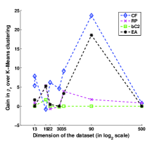
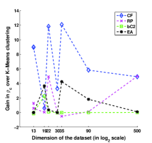
We define the feature profile plot to be the histogram of the strengths of each individual feature, where feature strength is defined as the $\kappa$ value computed on the dataset using this feature alone. (For categorical variables when the number of categories on this variable is smaller than the number of clusters, the strength of this feature is sampled at random from the set of strengths of other features.) Figure 5 shows the feature profile plot of the eight UC Irvine datasets used in our experiment. A close inspection of results presented shows that this plot can roughly guide us in choosing a “good” $q$ for each individual dataset. Thus a rule of thumb could be proposed: use large $q$ when there are many weak or noise features and the difference in strength among features is big; otherwise small $q$ or no feature competition at all. Alternatively, one could use some cluster quality measure to choose $q$. For example, we could use the $\kappa$ criterion as discussed in Section 2.1 or the Ncut value; we leave an exploration of this possibility to future work.

$q$	1	2	3	5	10	15	20
Soybean	92.36	92.32	94.42	93.89	93.14	94.54	94.74
SPECT	56.78	57.39	57.24	57.48	56.54	55.62	52.98
ImgSeg	79.71	77.62	77.51	81.17	82.69	83.10	82.37
Heart	56.90	60.08	62.51	63.56	63.69	63.69	63.69
Wine	79.70	74.02	72.16	71.87	71.87	71.87	71.87
WDBC	79.93	79.94	79.54	79.41	78.90	78.64	78.50
Robot	63.60	63.86	64.13	64.75	65.62	65.58	65.47
Madelon	50.76	50.94	50.72	50.68	50.52	50.40	50.38

Table 4: The $\rho_{r}$ achieved by CF for $q\in\{1,2,3,5,10,15,20\}$. Results averaged over $100$ runs. Note the first row is taken from Table 2.

$q$	1	2	3	5	10	15	20
Soybean	84.43	84.91	89.85	89.13	88.40	90.96	91.91
SPECT	68.02	68.90	68.70	68.67	66.99	65.15	60.87
ImgSeg	48.24	43.41	41.12	47.92	49.77	49.65	52.79
Heart	68.26	72.20	74.93	76.13	76.30	76.30	76.30
Wine	79.19	72.45	70.52	70.22	70.22	70.22	70.22
WDBC	88.70	88.71	88.45	88.37	88.03	87.87	87.75
Robot	41.20	40.03	39.57	39.82	38.40	37.73	37.68
Madelon	55.12	55.43	54.97	54.92	54.08	53.57	53.57

Table 5: The $\rho_{c}$ achieved by CF for $q\in\{1,2,3,5,10,15,20\}$. Results averaged over $100$ runs. Note the first row is taken from Table 3.

Additionally, we also explore the effect of varying $n_{b}$, and substantial performance gain is observed in some cases. For example, setting $n_{b}=10$ boosts the performance of CF on ImgSeg to $(\rho_{c},\rho_{r})=(62.34,85.92)$, while $n_{b}=3$ on SPECT and WDBC leads to improved $(\rho_{c},\rho_{r})$ at $(71.76,59.45)$ and $(90.00,82.04)$, respectively. The intuition is that the initial clustering by the base clustering algorithm may serve as a pre-grouping of neighboring data points and hence achieves some regularization with an improved clustering result. However, a conclusive statement on this awaits extensive future work.

5.2.1 Comparison to K-means clustering and spectral clustering

We have demonstrated empirically that CF compares very favorably to the three other clustering ensemble algorithms (i.e., RP, bC2 and EA). One might be interested in how much improvement CF achieves over the base clustering algorithm, $K$-means clustering, and how CF compares to some of the “best”

Figure 5: The feature profile plot for the eight UC Irvine datasets.

clustering methods currently available, such as spectral clustering. To explore this issue, we compared CF to $K$-means clustering and the NJW spectral clustering algorithm (see [32]) on the eight UC Irvine datasets described in Table 1. To make the comparison with $K$-means clustering more robust, we run $K$-means clustering under two different settings, denoted as $K$-means-1 and $K$-means-2, where $(n_{it},n_{rst})$ are taken as $(200,20)$ and $(1000,100)$, respectively. For the NJW algorithm, function specc() of the R project package “kernlab” ([26]) is used with the Gaussian kernel and an automatic search of the local bandwidth parameter. We report results under the two different clustering metrics, $\rho_{c}$ and $\rho_{r}$, in Table 6. It can be seen that CF improves over $K$-means clustering on almost all datasets and the performance gain is substantial in almost all cases. Also, CF outperforms the NJW algorithm on five out of the eight datasets.

Dataset	CF	NJW	K-means-1	K-means-2
Soybean	92.36	83.72	83.16	83.16
	84.43	76.60	72.34	72.34
SPECT	56.78	53.77	50.58	50.58
	68.02	64.04	56.18	56.18
ImgSeg	79.71	82.48	81.04	80.97
	48.24	53.38	48.06	47.21
Heart	56.90	51.82	51.53	51.53
	68.26	60.00	59.25	59.25
Wine	79.70	71.91	71.86	71.86
	79.19	70.78	70.23	70.22
WDBC	79.93	81.10	75.03	75.03
	88.70	89.45	85.41	85.41
Robot	63.60	69.70	39.76	39.76
	41.20	42.68	35.37	35.37
Madelon	50.76	49.98	49.98	49.98
	55.12	50.55	50.20	50.20

Table 6: Performance comparison between CF, spectral clustering, and K-means clustering on the eight UC Irvine datasets. The performance of CF is simply taken for $q=1$. The two numbers in each entry indicate $\rho_{r}$ and $\rho_{c}$, respectively.

6 Conclusion

We have proposed a new method for ensemble-based clustering. Our experiments show that CF compares favorably to existing clustering ensemble methods, including bC2, evidence accumulation and RP. The improvement of CF over the base clustering algorithm (i.e., $K$-means clustering) is substantial, and CF can boost the performance of $K$-means clustering to a level that compares favorably to spectral clustering. We have provided supporting theoretical analysis, showing that CF with $\kappa$ is “noise-resistant” under a simplified model. We also obtain a closed-form formula for the mis-clustering rate of spectral clustering which yields new insights into the nature of spectral clustering, in particular it underscores the importance of the relative size of clusters to the performance of spectral clustering.

7 Appendix

In this appendix, Section 7.2 and Section 7.3 are devoted to the proof of Theorem 1 and Theorem 2, respectively. Section 7.1 deals with the equivalence, in the population, of the optimal clustering rule (as defined by equation (4) in Section 4.1 of the main text) and $K$-means clustering. This is to prepare for the proof of Theorem 1 and is of independent interest (e.g., it may help explain why $K$-means clustering may be competitive on certain datasets in practice).

7.1 Equivalence of $K$-means clustering and the optimal clustering rule for mixture of spherical Gaussians

We first state and prove an elementary lemma for completeness.

Lemma 1.

For the Gaussian mixture model defined by (2) (Section 4.1) with $\Sigma=\bm{I}$ and $\pi=1/2$, in the population the decision rule induced by $K$-means clustering (in the sense of Pollard) is equivalent to the optimal rule $h^{*}$ as defined in (4) (Section 4.1).

Proof.

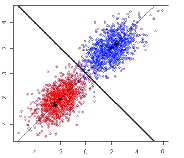
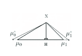
The geometry underlying the proof is shown in Figure 6. Let $\mu_{0},\Sigma_{0}$ and $\mu_{1},\Sigma_{1}$ be associated with the two mixture components in (2). By shift-invariance and rotation-invariance (rotation is equivalent to an orthogonal transformation which preserves clustering membership for distance-based clustering), we can reduce to the $\mathbb{R}^{1}$ case such that $\bm{\mu}_{0}=(\mu_{0}[1],0,...0)=-\bm{\mu}_{1}$ with $\Sigma_{0}=\Sigma_{1}=\bm{I}$. The rest of the argument follows from geometry and the definition of $K$-means clustering, which assigns $X\in\mathbb{R}^{d}$ to class $1$ if $||X-\mu_{1}^{*}||<||X-\mu_{0}^{*}||$, and the optimal rule $h^{*}$ which determines $X\in\mathbb{R}^{d}$ to be in class 1 if

$$(\mu_{1}-\mu_{0})^{T}(X-\frac{\mu_{0}+\mu_{1}}{2})>0,$$

or equivalently,

$$||X-\mu_{1}||<||X-\mu_{0}||.$$

∎

Figure 6: The optimal rule $h^{*}$ and the $K$-means rule. In the left panel, the decision boundary (the thick line) by $h^{*}$ and that by $K$-means completely overlap for a 2-component Gaussian mixture with $\Sigma=c\bm{I}$. The stars in the figure indicate the population cluster centers by $K$-means. The right panel illustrates the optimal rule $h^{*}$ and the decision rule by $K$-means where $K$-means compares $||X-\mu_{0}^{*}||$ against $||X-\mu_{1}^{*}||$ while $h^{*}$ compares $||H-\mu_{0}||$ against $||H-\mu_{1}||$.

7.2 Proof of Theorem 1

Proof of Theorem 1.

Let $\mathcal{C}_{1}$ and $\mathcal{C}_{0}$ denote the two clusters obtained by $K$-means clustering. Let $G$ be the distribution function of the underlying data.

$SS_{W}$ and $SS_{B}$ can be calculated as follows.

$$SS_{W} = \frac{1}{2}\int_{x\neq y\in\mathcal{C}_{1}}||x-y||^{2}dG(x)dG(y)+\frac{1}{2}\int_{x\neq y\in\mathcal{C}_{0}}||x-y||^{2}dG(x)dG(y)\triangleq(\sigma^{*}_{d})^{2},$$

$$SS_{B} = \int_{x\in\mathcal{C}_{1}}\int_{y\in\mathcal{C}_{0}}||x-y||^{2}dG(y)dG(x)=(\sigma^{*}_{d})^{2}+\frac{1}{4}||\mu_{0}^{*}-\mu_{1}^{*}||^{2}.$$

If we assume $\Sigma=\bm{I}_{p\times p}$ is always true during the growth of the clustering vector (this holds if duplicated features are excluded), then

$$\frac{1}{\kappa}=\frac{SS_{B}}{SS_{W}}=1+\frac{||\mu_{0}^{*}-\mu_{1}^{*}||^{2}}{4(\sigma^{*}_{d})^{2}}.$$ (11)

Without loss of generality, let $\mathcal{I}=\{1,2,...,d-1\}$ and let the noise feature be the $d^{th}$ feature. By the equivalence, in the population, of $K$-means clustering and the optimal clustering rule $h^{*}$ (Lemma 1 in Section 7.1) for a mixture of two spherical Gaussians, $K$-means clustering assigns $x\in\mathbb{R}^{d}$ to $\mathcal{C}_{1}$ if

$$||x-\mu_{1}||<||x-\mu_{0}||,$$

which is equivalent to

$$\sum_{i=1}^{d-1}\left(x[i]-\mu_{1}[i]\right)^{2}<\sum_{i=1}^{d-1}\left(x[i]-\mu_{0}[i]\right)^{2}.$$ (12)

This is true since $\mu_{0}[d]=\mu_{1}[d]=0$ by the assumption that the $d^{th}$ feature is a noise feature. (12) implies that the last coordinate of the population cluster centers for $\mathcal{C}_{1}$ and $\mathcal{C}_{2}$ are the same, that is, $\mu_{1}^{*}[d]=\mu_{0}^{*}[d]$. This is because, by definition, $\mu_{i}^{*}[j]=\int_{x\in\mathcal{C}_{i}}x[j]dG(x)$ for $i=0,1$ and $j=1,...,d$. Therefore adding a noise feature does not affect $||\mu_{0}^{*}-\mu_{1}^{*}||^{2}$. However, the addition of a noise feature would increase the value of $(\sigma^{*}_{d})^{2}$, it follows that $\kappa$ will be increased by adding a noise feature. ∎

7.3 Proof of Theorem 2

Proof of Theorem 2..

To simplify the presentation, some lemmas used here (Lemma 2 and Lemma 3) are stated after this proof.

It can be shown that

$$D^{-1/2}\overline{P}D^{-1/2} = \sum_{i=1}^{2}\lambda_{i}\mathbf{x}_{i}\mathbf{x}_{i}^{T},$$

where $\lambda_{i}$ are the eigenvalues and $\mathbf{x}_{i}$ eigenvectors, $i=1,2$, such that for $\nu=o(1)$,

$$\lambda_{1} = 1+O_{p}(\nu^{2}+n^{-1}),$$

$$\lambda_{2} = 1-\gamma^{-1}(1+\gamma^{2})\nu+O_{p}(\nu^{2}+n^{-1})$$

and

$$(n_{1}\gamma^{-1}+n_{2})^{1/2}\mathbf{x}_{1}[i]=\left\{\begin{array}[]{ll}\gamma^{-1/2}+O_{p}(\nu+n^{-1/2}),&~{}\mbox{if}~{}i\leq n_{1}\vspace{1pt}\\ 1+O_{p}(\nu+n^{-1/2}),&~{}\mbox{otherwise}.\end{array}\right.$$

$$(n_{1}\gamma^{3}+n_{2})^{1/2}\mathbf{x}_{2}[i]=\left\{\begin{array}[]{ll}-\gamma^{3/2}+O_{p}(\nu+n^{-1/2}),&~{}\mbox{if}~{}i\leq n_{1}\vspace{1pt}\\ 1+O_{p}(\nu+n^{-1/2}),&~{}\mbox{otherwise}.\end{array}\right.$$

By Lemma 3, we have $||\varepsilon||_{2}=O_{p}(\sqrt{n})$ and thus the $i^{th}$ eigenvalues of $D^{-1/2}PD^{-1/2}$ for $i\geq 3$ are of order $O_{p}(n^{-1/2})$. Note that, in the above, all residual terms are uniformly bounded w.r.t. $n$ and $\nu$.

Let

$$\psi = \frac{1}{2\pi i}\int_{\Gamma}(tI-D^{-1/2}PD^{-1/2})^{-1}dt,$$

where $\Gamma$ is a Jordan curve enclosing only the first two eigenvalues. Then, by (8) and (9) in the main text (see Section 4.2), $\psi\mathbf{x}_{2}$ is the second eigenvector of $D^{-1/2}PD^{-1/2}$ and the mis-clustering rate is given by

$$\mathcal{M}=\frac{1}{n}\left[\sum_{i\leq n_{1}}I((\psi\mathbf{x}_{2})[i]<0)+\sum_{i>n_{1}}I((\psi\mathbf{x}_{2})[i]>0)\right].$$

Thus

$$\mathbb{E}\mathcal{M}=\frac{1}{1+\gamma}\big{[}\mathbb{P}((\psi\mathbf{x}_{2})[i]>0)+\gamma\mathbb{P}((\psi\mathbf{x}_{2})[i]<0)\big{]}.$$

By Lemma 2 and letting $\tilde{\varepsilon}=D^{-1/2}\varepsilon D^{-1/2}$, we have

$$\psi\mathbf{x}_{2} = \frac{1}{2\pi i}\int_{\Gamma}\left(tI-D^{-1/2}\overline{P}D^{-1/2}-\tilde{\varepsilon}\right)^{-1}\mathbf{x}_{2}dt$$

$$= \frac{1}{2\pi i}\int_{\Gamma}\left(I-(tI-D^{-1/2}\overline{P}D^{-1/2})^{-1}\tilde{\varepsilon}\right)^{-1}\left(tI-D^{-1/2}\overline{P}D^{-1/2}\right)^{-1}\mathbf{x}_{2}dt$$

$$= \frac{1}{2\pi i}\int_{\Gamma}\left(I-(tI-D^{-1/2}\overline{P}D^{-1/2})^{-1}\tilde{\varepsilon}\right)^{-1}\mathbf{x}_{2}(t-\lambda_{2})^{-1}dt$$

$$= \phi\mathbf{x}_{2}+O_{p}(n^{-2}),$$

where

$$\phi\mathbf{x}_{2} = \frac{1}{2\pi i}\int_{\Gamma}\left[I+(tI-D^{-1/2}\overline{P}D^{-1/2})^{-1}\tilde{\varepsilon}\right]\mathbf{x}_{2}(t-\lambda_{2})^{-1}dt.$$

It can be shown that, by the Cauchy Integral Theorem [35] and Lemma 2,

$$\phi\mathbf{x}_{2} = \mathbf{x}_{2}+\frac{1}{2\pi i}\int_{\Gamma}\left(tI-D^{-1/2}\overline{P}D^{-1/2}\right)^{-1}\tilde{\varepsilon}\mathbf{x}_{2}(t-\lambda_{2})^{-1}dt$$

$$= \mathbf{x}_{2}-\lambda_{2}^{-1}\tilde{\varepsilon}\mathbf{x}_{2}+O_{p}(n^{-2}).$$

Let $\tilde{\varepsilon}_{i}$ be the $i^{th}$ column of $\tilde{\varepsilon}$. By Slutsky’s Theorem, one can verify that

$$\tilde{\varepsilon}_{1}^{T}\mathbf{x}_{2} = \sigma(n_{1}n_{2})^{-1/2}\mathcal{N}\left(0,\frac{1+\gamma^{3}}{1+\gamma^{2}}\right)+O_{p}(n^{-2}),$$

and

$$\tilde{\varepsilon}_{n}^{T}\mathbf{x}_{2} = n_{2}^{-1}\sigma\mathcal{N}\left(0,\frac{1+\gamma^{3}}{1+\gamma^{2}}\right)+O_{p}(n^{-2}).$$

Thus

$$\mathbb{P}((\psi\mathbf{x}_{2})[1]<0) = \mathbb{P}\left(\mathcal{N}(0,1)>(n_{1}n_{2})^{1/2}\sigma^{-1}\sqrt{\frac{1+\gamma^{2}}{1+\gamma^{3}}}\frac{\gamma^{3/2}}{\sqrt{n_{1}\gamma^{3}+n_{2}}}\right)(1+o(1))$$

$$= \mathbb{P}\left(\mathcal{N}(0,1)>n^{1/2}\sigma^{-1}\sqrt{\frac{\gamma^{2}}{(1+\gamma)(1+\gamma^{3})}}\right)(1+o(1)),$$

and

$$\mathbb{P}((\psi\mathbf{x}_{2})[1]>0) = \mathbb{P}\left(\mathcal{N}(0,1)>n_{2}\sigma^{-1}\sqrt{\frac{1+\gamma^{2}}{1+\gamma^{3}}}\frac{1}{\sqrt{n_{1}\gamma^{3}+n_{2}}}\right)(1+o(1))$$

$$= \mathbb{P}\left(\mathcal{N}(0,1)>n^{1/2}\sigma^{-1}\sqrt{\frac{\gamma}{(1+\gamma)(1+\gamma^{3})}}\right)(1+o(1)).$$

Hence

$$\lim_{n\rightarrow\infty}\frac{1}{n}\log(\mathbb{E}\mathcal{M}) = -\frac{\gamma^{2}}{2\sigma^{2}(1+\gamma)(1+\gamma^{3})},$$

and the conclusion follows. ∎

Lemma 2.

Let $\overline{P},\mathbf{x}_{2}$, $\lambda_{2}$, $\psi$, $\phi$ be defined as above. Then

$$\left(tI-D^{-1/2}\overline{P}D^{-1/2}\right)^{-1}\mathbf{x}_{2} = (t-\lambda_{2})^{-1}\mathbf{x}_{2},$$

and

$$||\psi\mathbf{x}_{2}-\phi\mathbf{x}_{2}||_{\infty} = O_{p}(n^{-2}).$$

The first part follows from a direct calculation and the proof of the second relies on the semi-circle law. The technical details are omitted.

Lemma 3.

Let $\varepsilon=\{\varepsilon_{ij}\}_{i,j=1}^{n}$ be a symmetric random matrix with $\varepsilon_{ij}\sim\mathcal{N}(0,1)$, independent for $1\leq i\leq j\leq n.$ Then

$$||\varepsilon||_{2} = O_{p}(\sqrt{n}).$$

The proof is based on the moment method (see [16]) and the details are omitted.

References

- [1] D. Achlioptas and F. McSherry. On spectral learning of mixtures of distributions. In Eighteenth Annual Conference on Computational Learning Theory (COLT), pages 458–469, 2005.
- [2] E. Airoldi, D. Blei, S. Fienberg, and E. Xing. Mixed membership stochastic blockmodels. Journal of Machine Learning Research, 9:1981–2014, 2008.
- [3] A. Asuncion and D. Newman. UC Irvine Machine Learning Repository. http://www.ics.uci.edu/ mlearn/MLRepository.html, 2007.
- [4] Y. Azar, A. Fiat, A. Karlin, F. McSherry, and J. Saia. Spectral analysis of data. In ACM Symposium on the Theory of Computing, pages 619–626, 2001.
- [5] J. Azimi and X. Fern. Adaptive cluster ensemble selection. In International Joint Conference on Artificial Intelligence, pages 992–997, 2009.
- [6] P. Bickel and A. Chen. A nonparametric view of network models and Newman-Girvan and other modularities. Proceedings of the National Academy of Sciences, 106(50):21068–21073, 2009.
- [7] L. Breiman. Random Forests. Machine Learning, 45(1):5–32, 2001.
- [8] R. Caruana, A. Niculescu, G. Crew, and A. Ksikes. Ensemble selection from libraries of models. In The International Conference on Machine Learning, pages 137–144, 2004.
- [9] S. Dasgupta. Experiments with random projection. In Uncertainty in Artificial Intelligence: Proceedings of the 16th Conference (UAI), pages 143–151, 2000.
- [10] D. L. Donoho. Compressed sensing. IEEE Transactions on Information Theory, 52(4):1289–1306, 2006.
- [11] S. Dudoit and J. Fridlyand. Bagging to improve the accuracy of a clustering procedure. Bioinformatics, 19(9):1090–1099, 2003.
- [12] X. Fern and C. Brodley. Random projection for high dimensional data clustering: A cluster ensemble approach. In Proceedings of the 20th International Conference on Machine Learning (ICML), pages 186–193, 2003.
- [13] X. Fern and W. Lin. Cluster ensemble selection. Statistical Analysis and Data Mining, 1:128–141, 2008.
- [14] A. Fred and A. Jain. Data clustering using evidence accumulation. In Proceedings of the International Conference on Pattern Recognition (ICPR), pages 276–280, 2002.
- [15] A. Fred and A. Jain. Combining multiple clusterings using evidence accumulation. IEEE Transactions on Pattern Analysis and Machine Intelligence, 27(6):835–850, 2005.
- [16] Z. Furedi and J. Komlos. The eigenvalues of random symmetric matrices. Combinatorica, 1:233–241, 1981.
- [17] A. Gionis, H. Mannila, and P. Tsaparas. Cluster aggregation. In International Conference on Data Engineering, pages 341–352, 2005.
- [18] J. A. Hartigan and M. A. Wong. A K-means clustering algorithm. Applied Statistics, 28:100–108, 1979.
- [19] T. Hastie, R. Tibshirani, and J. Friedman. The Elements of Statistical Learning: Data Mining, Inference, and Prediction. Springer, New York, 2009.
- [20] C. Hegde, M. Wakin, and R. Baraniuk. Random projections for manifold learning. In Neural Information Processing Systems (NIPS), pages 641–648, 2007.
- [21] P. Holland, K. Laskey, and S. Leinhardt. Stochastic blockmodels: Some first steps. Social Networks, 5:109–137, 1983.
- [22] L. Huang, D. Yan, M. I. Jordan, and N. Taft. Spectral clustering with perturbed data. In Neural Information Processing Systems (NIPS), volume 21, pages 705–712, 2009.
- [23] P. Huber. Projection pursuit. Annals of Statistics, 13:435–475, 1985.
- [24] A. Jain, M. Murty, and P. Flynn. Data clustering: a review. ACM Computing Surveys, 31(3):264–323, 1999.
- [25] R. Kannan, S. Vempala, and A. Vetta. On clusterings: Good, bad and spectral. Journal of the ACM, 51(3):497–515, 2004.
- [26] A. Karatzoglou, A. Smola, and K. Hornik. kernlab: Kernel-based Machine Learning Lab. http://cran.r-project.org/web/packages/kernlab/index.html, 2013.
- [27] T. Kato. Perturbation Theory for Linear Operators. Springer, Berlin, 1966.
- [28] M. Meila and J. Shi. Learning segmentation by random walks. In Neural Information Processing Systems (NIPS), pages 470–477, 2001.
- [29] M. Meila, S. Shortreed, and L. Xu. Regularized spectral learning. Technical report, Department of Statistics, University of Washington, 2005.
- [30] B. Minaei, A. Topchy, and W. Punch. Ensembles of partitions via data resampling. In Proceedings of International Conference on Information Technology, pages 188–192, 2004.
- [31] B. Nadler, S. Lafon, and R. Coifman. Diffusion maps, spectral clustering and eigenfunctions of Fokker-Planck operators. In Neural Information Processing Systems (NIPS), volume 18, pages 955–962, 2005.
- [32] A. Ng, M. I. Jordan, and Y. Weiss. On spectral clustering: analysis and an algorithm. In Neural Information Processing Systems (NIPS), volume 14, pages 849–856, 2002.
- [33] K. Nowicki and T. Snijders. Estimation and prediction for stochastic blockstructures. Journal of the American Statistical Association, 96:1077–1087, 2001.
- [34] D. Pollard. Strong consistency of K-means clustering. Annals of Statistics, 9(1):135–140, 1981.
- [35] W. Rudin. Real and Complex Analysis (Third Edition). McGraw-Hill, 1986.
- [36] J. Shi and J. Malik. Normalized cuts and image segmentation. IEEE Transactions on Pattern Analysis and Machine Intelligence, 22(8):888–905, 2000.
- [37] T. Shi and S. Horvath. Unsupervised learning with random forest predictors. Journal of Computational and Graphical Statistics, 15(1):118–138, 2006.
- [38] A. Strehl and J. Ghosh. Cluster ensembles: A knowledge reuse framework for combining multiple partitions. Journal of Machine Learning Research, 3:582–617, 2002.
- [39] A. Topchy, A. Jain, and W. Punch. Combining multiple weak clusterings. In Proceedings of the IEEE International Conference on Data Mining, pages 331–338, 2003.
- [40] S. Vempala and G. Wang. A spectral algorithm for learning mixture models. Journal of Computer and System Sciences, 68:841–860, 2004.
- [41] U. von Luxburg. A tutorial on spectral clustering. Statistics and Computing, 17:395–416, 2007.
- [42] U. von Luxburg, M. Belkin, and O. Bousquet. Consistency of spectral clustering. Annals of Statistics, 36(2):555–586, 2008.
- [43] D. Yan, L. Huang, and M. I. Jordan. Fast approximate spectral clustering. In Proceedings of the 15th ACM SIGKDD International Conference on Knowledge Discovery and Data Mining, pages 907–916, 2009.
- [44] Z. Zhang and M. I. Jordan. Multiway spectral clustering: A margin-based perspective. Statistical Science, 23:383–403, 2008.