Luminosity Functions and Point Source Properties from Multiple Chandra Observations of M81

Abstract

We present an analysis of 15 Chandra observations of the nearby spiral galaxy M81 taken over the course of six weeks in May–July 2005. Each observation reaches a sensitivity of $\sim 10^{37}$ erg s^-1. With these observations and one previous deeper Chandra observation, we compile a master source list of 265 point sources, extract and fit their spectra, and differentiate basic populations of sources through their colors. We also carry out variability analyses of individual point sources and of X-ray luminosity functions in multiple regions of M81 on timescales of days, months, and years. We find that, despite measuring significant variability in a considerable fraction of sources, snapshot observations provide a consistent determination of the X-ray luminosity function of M81. We also fit the X-ray luminosity functions for multiple regions of M81 and, using common parametrizations, compare these luminosity functions to those of two other spiral galaxies, M31 and the Milky Way.

1. Introduction

Deep X-ray observations of nearby galaxies allow for the study of their X-ray point source populations in considerable detail. Previous studies of a variety of different nearby galaxies have been able to probe these sources individually by measuring their spectral characteristics and luminosity variability over many different timescales. Populations of sources can also be scrutinized by the spatial and hardness distributions of sources and their X-ray luminosity function (XLF).

Fabbiano & White (2006) review the X-ray point source populations of numerous, nearby, star-forming galaxies. One of the most notable is M31 because of its proximity and general similarities to the Milky Way. Because M31 is the closest large spiral galaxy, numerous studies have analyzed the X-ray point source populations in great detail with past and current X-ray observatories: Einstein (Trinchieri & Fabbiano, 1991), ROSAT (Primini et al., 1993; Supper et al., 1997), Beppo Sax (Trinchieri et al., 1999), Chandra (Kong et al., 2003), and XMM-Newton (Shaw Greening et al., 2009). The two most recent observations with XMM-Newton and Chandra, in particular, contain the best data yet, but only in small segments of the galaxy at a time because the spatial extent of the galaxy is much larger than the fields of view of these current X-ray telescopes.

In the last decade, the X-ray point source populations of many other nearby, star-forming galaxies have also been scrutinized: late-type spiral galaxies, irregular galaxies, and merging galaxies. Not long after the launch of the Chandra and XMM-Newton space telescopes, Soria & Kong (2002), Soria & Wu (2002), and Pence et al. (2001) observed the X-ray point source populations of M74, M83 and M101, respectively, all Sc-type spiral galaxies. More recently, the ChaseM33 survey observed the X-ray point source populations of another Sc-type galaxy, M33 (Plucinsky et al., 2008; Williams et al., 2008), and Fridriksson et al. (2008) completed a study of the X-ray point source populations of a pair of galaxies, NGC 6946 (Sc-type) and NGC 4485/4490 (an irregular galaxy). In addition, in a series of papers, Zezas et al. (2002); Zezas & Fabbiano (2002); Zezas et al. (2006, 2007) studied the X-ray point source population in the unique environment of the merging Antennae galaxies.

X-ray point source populations from predominantly old stellar populations of early-type galaxies, have also been examined. In the S0 galaxy, NGC 1553, Blanton et al. (2001) found that most of the X-ray emission is diffuse, with 49 sources comprising only 30% of the light. The rest of the galaxies mentioned here are among the many optically bright elliptical galaxies associated with nearby galaxy clusters. NGC 4697 and NGC 4472 (M49), two large elliptical galaxies in the Virgo cluster, have been observed with Chandra. Detailed analysis of NGC 4697 by Sarazin et al. (2000) resolved almost all of the hard emission and a large fraction of the soft emission into 90 point sources, most of which are expected to be low-mass X-ray binaries (LMXBs). Also, Kundu et al. (2002) and Maccarone et al. (2003) analyzed the X-ray point source population of NGC 4472 and found 144 point sources. Lastly, a Chandra observation of the bright central galaxy in the Fornax cluster, NGC 1399, revealed 214 point sources (Angelini et al., 2001).

From these and other studies of old stellar populations, general trends have been discerned in the X-ray populations. In the XLFs of X-ray point source populations of elliptical galaxies, there is evidence for a varying break and varying slopes on either side of the break (e.g., Kim & Fabbiano, 2010). There is also evidence for differences between the XLFs of field and cluster binaries (Fabbiano et al., 2010). Particularly prevalent in the X-ray observations of large elliptical galaxies is the large fraction of globular cluster sources (e.g., $\lesssim 70\%$ of the sources in NGC 1399; Angelini et al., 2001). By matching Chandra and HST observations, possible trends in the populations can be explored (e.g., metallicity).

In these many X-ray observations of early- and late-type galaxies, these authors inspect the X-ray point sources populations from a variety of perspectives. Hardness ratios are frequently calculated (albeit in a number of different ways). They are most often used to differentiate populations of sources within each galaxy but have been also used to differentiate galactic sources from background active galactic nuclei (AGN). The most luminous or most unusual sources in each of the galaxies are typically of particular interest: ultra-luminous X-ray sources (ULXs), transient sources, or supersoft sources (SSSs). They are frequently examined in detail in terms of their spectral characteristics and spectral and flux variability.

When X-ray point source populations are inspected using XLFs of different galaxy types and stellar population ages (i.e., actively star-forming versus relatively quiescent), considerable variation has been observed. High-mass X-ray binary (HMXB) XLFs, which are associated with regions of current star formation, are typically described by straight (unbroken) power laws. For simplicity, we refer to these as “disk-like” XLFs in this study. Typical cumulative slopes are $\sim-$0.7–1.0 for moderate star formation rates (SFRs; $\lesssim 1M_{\sun}$ yr^-1) and $\sim-$0.4–0.5 for higher SFRs (e.g., Kilgard et al., 2002; Grimm et al., 2002; Colbert et al., 2004). LMXB XLFs or what we refer to as “bulge-dominated” XLFs in this study are not associated with recent star formation. These XLFs are typically described by broken or cutoff power laws (e.g., Kim & Fabbiano, 2004; Gilfanov, 2004) with signs of a flat low-luminosity end and a break or cutoff at a few $\times\ 10^{38}$ erg s^-1, which is frequently attributed to the Eddington luminosity for a neutron star. Spiral galaxies (earlier type, in particular) show mixed XLFs with contributions from both types of XLFs, “disk-like” and “bulge-like”.

Developing physical models to describe the populations of galactic X-ray sources, which are the result of the evolution of their stellar populations, is a daunting task. Some studies have attempted to understand the star formation history of these galaxies through the use of population synthesis modeling. These complex models attempt to follow the stellar populations through many evolutionary phases to the formation of the X-ray bright systems that we observe (Belczynski et al., 2008). There also exist alternate, less complex, methods such as that of Wu et al. (2003) in a previous study of M81 and White & Ghosh (1998), who construct simple birth and death rate models for components of the stellar populations. However, accurately constructing XLFs to low luminosities and comparing them to models is very difficult (e.g., Fragos et al., 2008), and the information gleaned from doing this (e.g., finding and interpreting breaks in XLFs) can be ambiguous.

Some key questions concerning XLFs remain unanswered. For example, is there a break in the XLFs of spiral galaxies at low fluxes? Also, essentially every study of these types of X-ray point sources has noted a wide range of levels and timescales of both integrated flux variability and spectral variability. However, the XLFs of galaxies are almost always characterized by a single X-ray snapshot of the galaxy. A critical question can then be raised: does the variability of the individual sources significantly manifest itself in a variable XLF? In other words, is the XLF robust against the fluctuations of its constituents? Very large changes in the XLF over the timescales that we are probing, which are much shorter than stellar evolution timescales, should not be observed since this would require correlated variability of many sources. However, the stability of XLFs has not been thoroughly investigated over the days, weeks, and years timescales.

The nearby Sb-type galaxy, M81, with multiple types of X-ray binaries, is a key object with which to address these points and is an excellent choice for studying the X-ray point source population with Chandra. Because M81 is relatively nearby at a well-determined distance ($3.63\pm 0.34$ Mpc; Freedman et al. 1994; using the Cepheid period-luminosity relationship), we can detect sources with faint luminosities in relatively short exposures and calculate their luminosities accurately. However, M81 is at a large enough distance so that almost the entire galaxy fits within the field of view of Chandra in one exposure. These facts make it easy to use Chandra to study the variability characteristics of the X-ray point source population to relatively low luminosities ($\gtrsim 10^{37}$ erg s^-1) in a minimum amount of observations.

M81’s X-ray point source population has been scrutinized many times in the past. Fabbiano (1988) was the first to study the X-ray point source population of this galaxy with Einstein, but was only able to detect a handful of sources. Later on, Immler & Wang (2001) studied this galaxy with ROSAT and detected $\sim 5$ times as many sources to fainter luminosities. Most recently, Tennant et al. (2001) and Swartz et al. (2003) found 177 sources with Chandra in a single exposure, 17–27 of which are expected to be background AGN (e.g., Rosati et al., 2002). Out of these galactic sources, some are expected to be SNRs, ULXs, SSSs, or young pulsars/pulsar wind nebulae, but most are likely LMXBs and HMXBs.

We seek to follow-up the work of Tennant et al. (2001) and Swartz et al. (2003) and to add to the understanding of the characteristics of the X-ray point sources and XLFs of nearby galaxies by carrying out an observational study of the nearby galaxy M81. We use a set of sixteen Chandra observations of M81 that explore variability on timescales of days, weeks, and years. We also use these observations to make the most complete study of M81’s X-ray point source population to date.

In § 2, we lay out the observations and data reduction procedures. Then, in § 3, we discuss the creation of our point source catalogs. In § 4 and § 5, we present hardness ratios and discuss the individual variability of the point source population, respectively. Following this, we construct XLFs in § 6. Then, in § 7, we compare our results with M31 and the Milky Way. Finally, in § 8, we summarize our results and state our conclusions. For all of our analyses throughout this work, we use the energy range of 0.5–8.0 keV (e.g., fluxes, luminosities), unless otherwise noted.

2. Observations and Data Reduction

We present fifteen Chandra observations of M81 (ObsIDs 5935-5949) taken specifically to explore XLF and individual point source variability. For our analysis, we include an additional observation from the Chandra archive (ObsID 735 Tennant et al., 2001; Swartz et al., 2003) to provide a longer baseline for measuring variability (see Table 1). All sixteen observations were taken with the Advanced CCD Imaging Spectrometer (ACIS; Garmire et al. 2003) in Timed Exposure mode with a frame time of 3.2 s and the aimpoint on the default location of the S3 chip. The data were telemetered to the ground in Faint mode.

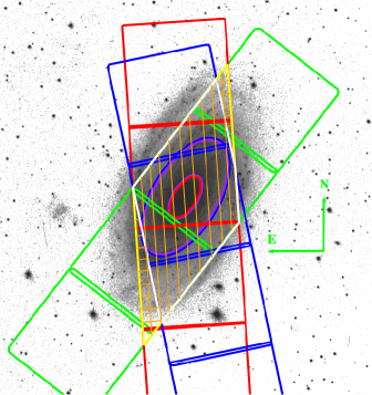
We analyze all of these observations using the CIAO software provided by the Chandra X-ray Center as well as the IDL-based ACIS Extract program version 2008-03-04 (AE; Broos et al. 2010). We ignore the ACIS-I chips for the entire analysis for three primary reasons: 1) the observations were purposely taken to line-up the galaxy on the ACIS-S chips so that any sources found on the ACIS-I chips are far less-likely to be associated with M81; 2) point source extractions for sources on chips I2 or I3 become very difficult because the CALDB PSF library that this version of AE uses for automated spectral extraction does not contain the appropriate PSFs; and 3) the PSF quickly becomes impractically large there. Our X-ray coverage of the galaxy is shown in Fig. 1.

Figure 1.— Overlaid on a blue POSS2 DSS image of M81 are the outlines of the positions of the ACIS-S chips to show where we have coverage in the 16 observations that we use. The blue boxes represent ObsID 735 and the red and green boxes represent ObsIDs 5935 and 5949 (the remainder of the 2005 observations were taken at intermediate roll angles). The overlapping sky coverage of the fifteen 2005 and all sixteen observations are represented by the yellow and white polygons (or regions of orange cross-hatch and vertical lines), respectively. The ellipses mark the separations between the bulge, inner disk, and outer disk regions (see § 4.1; the colors of the ellipses match the colors used for the sources in Fig. 5). The image is $\sim 30^{\prime}\times 30^{\prime}$.

Table 1Chandra Imaging Observations of M81

Start Date	Spacing†	Obs. ID	Exposure Time
	(days)		(s)
2000 May 7	——	735	50021
2005 May 26	1844.9	5935	10979
2005 May 28	2.7	5936	11406
2005 Jun 1	3.5	5937	12006
2005 Jun 3	2.6	5938	11807
2005 Jun 6	2.7	5939	11807
2005 Jun 9	2.7	5940	11974
2005 Jun 11	2.6	5941	11807
2005 Jun 15	3.2	5942	11952
2005 Jun 18	3.4	5943	12012
2005 Jun 21	2.7	5944	11807
2005 Jun 24	3.0	5945	11576
2005 Jun 26	2.7	5946	12019
2005 Jun 29	2.7	5947	10698
2005 Jul 3	3.5	5948	12028
2005 Jul 6	3.3	5949	12022

Note. — ($\dagger$) time since the prior observation

We checked the relative pointing of Chandra and found it to be quite good. We only found tiny relative, systematic offsets of not more than $0\farcs 05$ between the observations by comparing the positions (which were optimized with multiple iterations of AE’s CHECK_POSITIONS stage) of all of the point sources within 2^′ of the aimpoint at one time. We changed the WCS header information to account for these tiny offsets. Then, for all 16 observations, we reprocessed the level=1 event files with CIAO 4.0 following the threads on the Chandra X-ray Center website to apply the most-recent calibration updates available (CALDB version 3.5.0). We used all of the default “acis_process_events” parameters except the “rand_pix_size” keyword, which we set to 0. Monoenergetic exposure maps at 1.0 keV were created where needed for wavdetect and the AE analysis.

We inspected the total background for each observation and found background flares in ObsIDs 5936, 5945, 5946, and 5947. These flares will not affect our point source extractions (although they do affect our background model selection) because we always include a local background when fitting each source’s spectrum. Therefore, we did not exclude the time intervals of the flares in our observations.

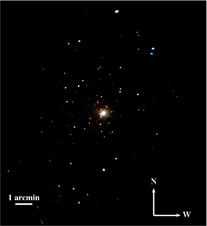
We also constructed a coadded observation of ObsIDs 5935–5949. We used the “merge_all” CIAO contributed script to coadd the event files and exposure maps for source detection and for the creation of Figure 2. Any other coadded source information was calculated for each observation with AE and then merged with AE’s MERGE_OBSERVATIONS step, which properly takes into account observation-to-observation instrumental details (i.e., weighting the data products appropriately). We refer to information gleaned from the combination of ObsIDs 5935–5949 as the “merged” observation information throughout this work.

Figure 2.— Three-color Chandra image of the merged observation. Photons in the 0.5–1 keV band (“soft”) are shown in red, those in the 1–2 keV band (“medium”) are shown in green, and those in the 2–8 keV band (“hard”) are shown in blue. The image is $12.4^{\prime}\times 14.4^{\prime}$.

3. Source Lists

3.1. Source Detection and Construction of the Master Source List

We used wavdetect (Freeman et al., 2002), CIAO’s wavelet source detection algorithm to search for sources in all of the individual observations as well our merged observation. It was not appropriate to include ObsID 735 in the merged observation for source detection because the aimpoint of this observation (very near to SN 1993J) is $\sim 2.8$ arcmin southwest of the aimpoint of ObsIDs 5935–5949 (very near the center of the galaxy). This means that the size and shape of the PSF is different in the same sections of the galaxy between ObsIDs 5935–5949 and 735, which would lead to less-efficient source detections.

We first filtered the ObsIDs to 0.5–6.0 keV to minimize noise. Then, we consistently searched for point sources on a chip-by-chip basis since the size and shape of the PSF changes as a function of off-axis angle. We used the default settings for the wavdetect parameters, where applicable (notably, the significance threshold, “sig_thresh”, was $10^{-6}$, which corresponds to approximately one spurious source per ACIS chip), except for the scales parameter. We searched a variety of spatial scales in a $\sqrt{2}$ series (as suggested in the wavdetect manual) using different upper and lower bounds for each chip. We searched scales of 2–8 pixels on S3, 2–16 pixels on S2, 6–34 pixels on S4, and 14-40 pixels on S1.

There were a number of complications that arose when constructing our master source list:

1. While matching sources between observations in crowded subfields at large off-axis angles, it was not always initially clear whether the apparently matched source was actually the same source or whether we were confusing multiple nearby sources. This is because the position uncertainty far off axis can be quite large, especially when the source is near the detection limit. Furthermore, source variability can cause some sources to become particularly dim or drop below the detection threshold in certain observations. As a remedy for most of the sources in this category, we considered two detected sources as one if their extraction regions, which enclose the inner 50% of the PSF, overlapped.

2. For a few sources at intermediate off-axis angles, PSF substructure also caused very close double source detections. Careful inspection of the PSFs for these few sources revealed that wavdetect finds two sources in one complicated PSF (see Kim et al. 2004, who provide details about this problem in their analysis for the ChaMP survey). While it is possible that, in these cases, the double sources are real, it is very unlikely and, following our rule in step 1., we would not be able to separate them anyway if they were real.

3. A considerable readout streak from M81*, the AGN in the low-ionization nuclear emission-line region (LINER) in the center of the galaxy, was present in all 16 observations, most significantly ObsID 735, causing wavdetect to find many false sources. We exclude M81* from our source lists. Sources on the readout streaks were considered real only if they were detected in multiple observations. We were able to make this cut since the read streak changed position on the sky with the changing roll angle of the telescope.

4. Obvious false detections, which include sources with only 1–2 counts were rejected. One false detection is expected per chip with the default wavdetect settings that we used.

5. The background in the center of M81 due to the wings of the PSF of M81*, unresolved galactic point sources, and diffuse galactic emission was non-uniform, quite high, and varied slightly in intensity in different positions on the chips, which made it difficult to detect sources. In this case, we used maximum likelihood reconstructions (constructed with multiple iterations of IDL’s “max_likelihood” routine–implemented with AE) of the region near M81*. Six additional sources and a severe surface brightness depression caused by pileup effects were detected in the neighborhood of M81*. Since these sources were embedded very near to this piled-up region and in a highly sloped background from a combination of wings of the PSF of M81* and M81’s galactic background, we do not include these sources in our master or borderline source lists (see below). Because of these complications, we were only able to reliably extract the wavdetect positions for these sources, which we list in Table 2.

Table 2Sources Near the Center of M81

Source	RA	Dec
number	(degrees)	(degrees)
ML1	148.88791	69.06654
ML2	148.88738	69.06575
ML3	148.89164	69.06485
ML4	148.89197	69.06385
ML5	148.88913	69.06377
ML6	148.88531	69.06648

Note. — Sources were found using maximum likelihood image reconstruction

In any of the source rejection steps above, if we were uncertain whether to keep the source or not, we kept it. Out of these first five source list refinement steps, most of the sources were removed in step 3.

1. We made one final cut on our preliminary source list using the AE’s PROB_NO_SOURCE statistic, which estimates whether a source is real by sampling the binomial probability distribution. We kept only sources at the 99.9% probability level of being real according to this statistic. Our final source list contains 265 sources which are listed in ancillary tables. We also include list of sources at the 99–99.9% probability level according to the PROB_NO_SOURCE statistic and deem these 11 sources “borderline sources” (referred to as B1-B11). Note that only coordinates are listed for three sources in the master source list and two sources in the borderline source list because they were only in the field of view (on chip) of ObsID 735: 234, 241, 262, B8, and B9.

Overall, this careful multiple-step approach to refining our master source list rejected $\sim 36\%$ of the original wavdetect sources as false detections.

Finally, we note that using the Chandra Point-Source Catalog (CSC) to construct source lists for M81 for simplicity is tempting, but would yield incomplete results. The current source list from the CSC contains $\lesssim 50\%$ of sources that we found in the galaxy through our more careful searching. Such a disparate result can be explained by the differences in how we and the CSC make use of wavdetect for the construction of our source lists (our numbered procedure above is very different than the CSC’s procedures). For example, the CSC uses different: wavelet scales, energy filtering, blocking, and significance thresholds. The most important difference to the overall process is that we have stacked our 15 new observations, revealing a multitude of additional, faint sources.

3.2. Point-Source Extraction with ACIS Extract

We used AE for the extraction of the source and background spectra. One of the primary reasons that we use AE (as opposed to other CIAO tools such as psextract) is that AE calculates the size, shape, and position of each extraction region, and it calculates the auxiliary response file (ARF) taking into account the PSF fraction enclosed in the region as a function of energy. We also use AE to refine the positions beyond the initial wavdetect estimates and calculate some useful statistics and photometry.

We briefly lay out the point source extraction process here. First, we constructed regions to match the PSF retreived from the CALDB library and that enclose a prescribed percentage of the PSF (90% default unless it needed to be adjusted to as low as 50% for nearby sources relative to the size of the PSF). Then for each point source, we extracted the source events within the PSF-matched region and a representative background in an annular region centered on the point source.

With this information, AE then provides new position estimates for each of the sources. We refined the positions of the sources according to the prescriptions in the AE manual. For sources that were $\leq 5^{\prime}$ from the aimpoint, we used the mean event position, and, for sources that were $>5^{\prime}$ from the aimpoint, we used the correlation position. The latter position is calculated automatically by AE, by correlating the neighborhood around the source (not just the extracted counts) with the source’s PSF. Since the positions of some of the sources (especially the fainter ones) take time to converge, we ran these first few steps a minimum of 5 times. This provides us with very accurate source positions, useful for comparing to observations taken with other telescopes and provides accurate flux estimates.

Lastly, we extracted the spectra for each source and its local background, which included the creation of the ARF and RMF (redistribution matrix file) files for fitting the spectra. AE implements rules so that the background is always well-constrained. At minimum, the background spectrum must always have at least 100 counts and a ratio of the photometric errors of the source to background of at least 4.0 (so that the error in the background does not dominate the total error). These constraints on the background extraction yielded a median background radius of 76 sky pixels with $>99\%$ of the sources having radii less than $\sim 200$ sky pixels and $<1\%$ of the sources farthest off-axis having radii of $\sim 200$–500 sky pixels.

3.3. Spectral Fitting and Source Properties

Figure 3.— Source hardness as a function of conversion factor from counts to ergs for sources in our merged master source list. The estimated source flux will be biased if a single conversion factor is used to convert counts to energy flux units. The vertical line of points near 3.3 represents the spectral fits where the photon index was frozen to 1.7 and N_H was frozen to or floated to the minimum value in the direction of M81. The points only extend $\sim 1$–11 on the x-axis because of the constraints imposed on the fit parameters, which are laid out in § 3.3. The hardness ratio for a photon index of 1.7 and a column density equal to the Galactic column density in the direction of M81 is $-0.39$ ((H$-$S)/T). H: 2–8 keV; S: 0.5–2 keV, T: 0.5–8 keV

Figure 4.— Distributions of the two key fit parameters for the fits of the merged spectra. The vertical line in the upper left plot is the weighted average photon index and the two curves are analytic fits to the $1\sigma$ uncertainties added to a natural width of the distribution. The natural width, 0.32, is calculated so that 68.3% of the points are within $1\sigma$ of the weighted average photon index.

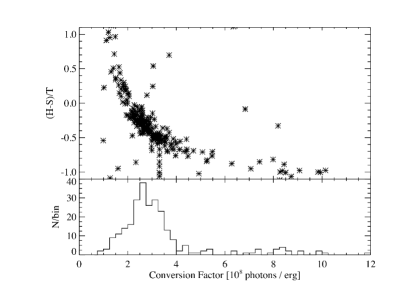
To estimate the energy fluxes and other source properties, we fit the source and background spectrum of each source in each observation ($\sim 4000$ spectra, most fit using automated methods detailed below). We tested an alternate method of estimating fluxes by using a single count-rate-to-flux conversion factor. We found that this would have led us to calculate different source fluxes by factors of order unity or less (see Fig. 3; see also § 7.2 for a brief discussion of this effect with regard to the XLFs). We jointly fit the unbinned source and background spectrum of each source in each observation in Sherpa (Freeman et al., 2001) using the C-statistic, which is similar to the Cash (1979) statistic but with an approximate goodness-of-fit measure, and the Powell minimization algorithm.

Since almost all of the sources have too few counts to constrain many of their source properties and since we are mainly interested in estimating accurate fluxes, we began by fitting the source and background spectra for each source in each observation with absorbed power-law models (xswabs $\times$ xspowerlaw). We initially used the default parameter boundaries (xswabs.nH=[0.01,10] ($10^{22}$ cm^-2), xspowerlaw.PhoIndx=[-3,10], xspowerlaw.norm is estimated from the data) in Sherpa in all cases except one. We always constrained the hydrogen column density to be at least that of the Milky Way in the direction of M81, $4.2\times 10^{20}$ cm^-2 (Dickey & Lockman, 1990).

Since degeneracies in the fit parameters will frequently arise for very faint sources, we followed a specialized scheme for these sources based on the number of counts in the source extraction region. If we extracted less than 5 counts (0.5-8 keV) for a source, the power-law index and the hydrogen column density for the fit were frozen to 1.7 and the Galactic value, respectively. If we extracted more than 5 but less than 26 counts (0.5-8 keV), we froze only the power-law index to 1.7 and let the hydrogen column density float, although, in this case, it was always poorly constrained. For all other sources with more than 26 counts (0.5-8 keV), we allowed all fit parameters to float.

Figure 5.— Hardness ratios for the merged observation plotted as in Prestwich et al. (2003) (H: 2–8 keV; M: 1–2 keV; S: 0.5–1 keV, T: 0.5–8 keV). The median Gehrels error bars for all of the sources are in the lower right corner of the plot. The dotted lines represent the physical boundaries, outside of which the number of net counts are negative. This can happen for very faint sources when the background is subtracted. Finally, note that a large percentage of the sources in this plot are likely background AGN (see Fig. 11), especially in the outer disk region, that usually cannot be separated from the other point sources in the galaxy using this classification scheme.

Following these rules, we obtained reasonable fits for most of the sources. However, some of the individual-observation source spectra ($\sim 17\%$), did not have acceptable fits using these rules alone. First, the background spectra were not always well-fit by a single absorbed power-law model. The merged spectra revealed that, when well-sampled, background spectra were always quite complicated. These complications exhibited themselves sometimes in the individual observation source spectra. For the cases where the reduced background goodness of fit statistic was $\geq 0.9$, a more complicated background model, two power laws and a blackbody (xswabs $\times$ (xspowerlaw $+$ xspowerlaw $+$ xsbbody)) was used to achieve a good fit. This ad hoc combination of models is only used to model the shape of the background spectra.

Second, there were some sources ($\lesssim 4$% of the fits) in which the best-fit hydrogen column density of the source was found at the maximum of the parameter space, $10^{23}$ cm^-2. Since the simple absorption model does not account for multiple photon scatterings through a Compton-thick medium and we did not consider other absorption models for our spectral fitting, we refit the spectra using a maximum hydrogen column density of $10^{24}$ cm^-2, which allowed for reasonable spectral fits for most of these sources. However, there were still a small subset of sources ($\lesssim 1$% of the fits) with 5–25 counts where the best-fit hydrogen column densities were at $10^{24}$ cm^-2. For these few sources, we allowed the power-law photon index, $\Gamma$, to float. This led to resonable fits for these sources.

Third, there were sources with best-fit power-law indices up to 10, the maximum parameter space boundary. For these soft sources with $\Gamma>3$ ($\lesssim 3$%), we changed the source model to a simple thermal (xsbbody) model and achieved good fits (C-statistic $\leq 1$ with kT $<$ 1 keV). Our change in spectral model here does not imply that there are not sources that could be well-fit by this model with temperatures in excess of 1 keV. Given the limited number of source counts for most sources, we expect that such sources were well-fit by the absorbed power-law model. This only implies that there were sources that could not be well-fit by the absorbed power-law model within a reasonable range of photon indices because their spectra were too soft. This result indicates that we cannot differentiate these models for most of our sources that are not very soft. This is acceptable since our goal is not to differentiate source models. These comments also apply to the merged spectra that are mentioned below.

Fourth, a very small number of sources ($\lesssim 1$%) had $\Gamma<0$ or had spectra such that Sherpa could not find a reasonable local minimum and frequently ran into parameter space boundaries. These were generally sources that had only a few counts, and were located in regions where the background spectrum was complicated. In these cases, the software had to be manually guided until a reasonable fit was found.

In summary, we allowed for fairly liberal upper and lower bounds for the fit parameters because there are a wide range of different types of sources in our sample (e.g., LMXBs, HMXBs, SNRs, SSSs, ULXs, background AGN, etc.). After considerable experimentation and iteration, the following constraints were imposed on our spectral fitting process:

1. We required the reduced goodness of fit statistic for the source to be better than 1.2.

2. We required the reduced goodness of fit statistic for the background to be better than 0.9 for sources within 7 arcmin of the aimpoint and better than 1.4 for sources farther off-axis than 7 arcmin.

3. The source absorption, N${}_{\text{H}}$, must be less than $10^{24}$ cm^-2 (the Compton-thick limit).

4. No sources can be very near to or stuck at parameter space boundaries.

5. The source power-law fits cannot have a photon index greater than 3 or less than 0.

6. The blackbody (thermal) fits were specifically implemented only for very soft sources and do not have kT greater than 1 keV.

At the end of the fitting process, all fits abided by these rules.

Out of all source fits in each of the 16 observations, two sources in ObsID 735 required special attention with the use of more complicated models. First, the brightest ULX (source 21) was the only source that suffered from significant pileup and, therefore, Sherpa’s JD pileup model (Davis, 2001) was used in addition to the power-law fit. The second source, SN1993J (the aim of ObsID 735), was fit by two low-temperature absorbed thermal emission-line (vmekal) components. Since care has already been taken in fitting these sources (Swartz et al., 2003), we used these models.

We also fit the source spectra of ObsIDs 5935–5949, the merged observation, to better understand the properties of each source. We did not include the ObsID 735 in the merged spectra because the ARF changes significantly and there appears to be spectral variability in at least a few sources (see § 5.2). We fit the merged source spectra with simple absorbed power-law models as above. We found that 219 of the 262 sources were well-fit by this method (CSTAT $\lesssim$ 1). Again, two sources (the brightest ULX and SN1993J) were fit with special models, as described in the previous paragraph. The remaining sources were better fit by simple blackbody (thermal) models. Almost all of the sources better fit with the simple thermal model also had hardness ratios indicative of thermal SNR or SSS populations (see § 4). In all cases, the background was poorly fit by a single absorbed power law. We used the more complicated background model expressed above, which achieved good fits.

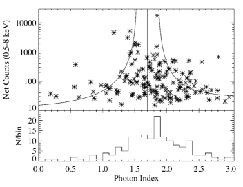
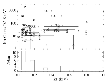
Fit parameter distributions are shown in Figure 4. There appears to be no correlation between the net counts and the blackbody temperature for the softest sources, although there is a lower cutoff in the blackbody temperature, which is likely due to the dropoff in sensitivity of Chandra at lower energies and foreground absorption. The distribution of photon indices can almost entirely be accounted for by the uncertainties in the photon indices ($\sim 68.3\%$ within $1\sigma$ of the mean) with a natural width of 0.32 to the distribution.

For each source in the master and borderline source lists, we compile one table for our merged source photometry and another for our merged spectral fits, which are both ancillary tables.

4. Hardness Ratios

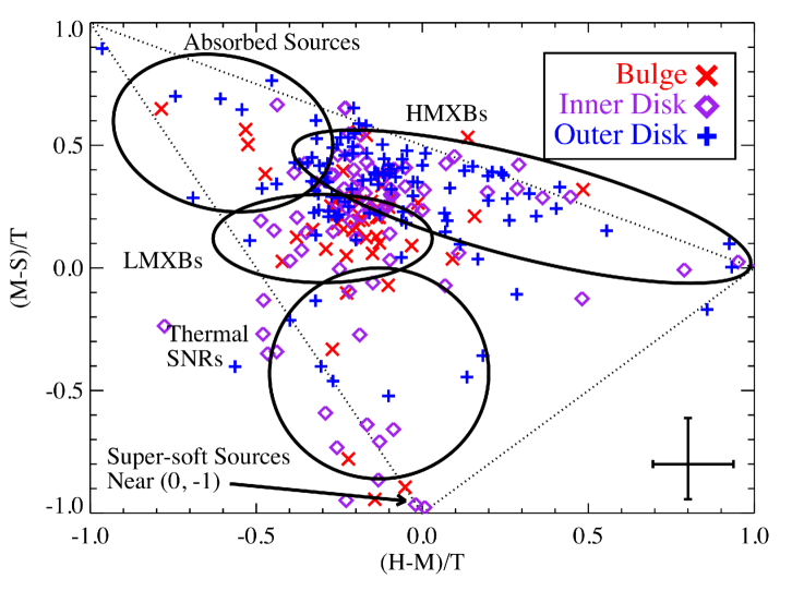
Following Prestwich et al. (2003), we calculate hardness ratios using the AE pipeline for the sources in our master source list (Fig. 5) from the background-subtracted counts of the merged observation in different bands (H: 2–8 keV; M: 1–2 keV; S: 0.5–1 keV, T: 0.5–8 keV). Since most of the sources have far too few counts to make significant statements about the source properties, we use these hardness ratios to estimate the spectral properties of the differing source populations in this dataset. The population of sources shows the full range of expected colors as seen in Fig. 5.

This classification is based on the general characteristics of the HMXB and LMXB populations in our Galaxy. The former are predominantly pulsar X-ray binaries and hence have hard spectra, while the latter host either black holes or low-magnetic field neutron stars resulting in softer spectra (at least at the luminosities that we are probing with these observations). HMXBs with black-holes could also be in the same locus but, in our Galaxy, these are substantially rarer than LMXBs. Given the similarity of M81 with our Galaxy, we would also expect that the vast majority of the objects in this locus are LMXBs. As was emphasized in Prestwich et al. (2003), the color of an individual source calculated in this fashion is not sufficient to determine the precise nature of the source. Instead, this color classification scheme is useful primarily for population studies, and we take advantage of this fact in the next section.

Further insight into the multi-wavelength properties of these sources requires detailed source matching with additional observations (e.g., optical observations), which is beyond the scope of this study. As a result, we cannot individually identify background AGN apart from galactic source populations in M81 at the present time. To varying degrees, this sometimes limits the interpretation of our: color-color analysis in this section, variability analysis in § 5, and interpretation and comparisons of the disk XLFs (mainly for the outer disk; § 6). Also, because of this and the fact that our monitoring observations mainly focus on the bulge and inner disk regions, we do not perform a spatial correlation analysis between the positions of the sources in M81 to the spiral arms of M81, which has been previously done (Swartz et al., 2003). Some of these tasks will be carried out in a future publication that will include detailed source matching with the deepest Hubble Space Telescope image to date (Zezas et al. in prep.). Despite these current limitations, we do carry out interesting spatial, variability, and XLF analysis in the later sections.

4.1. Separating the Bulge and Disk

Figure 6.— The number of observations that each source in the master source list in the field of view. There are a number of situations throughout this work where excluding sources not in the field of view of all 16 observations is appropriate for consistency.

In order to search for trends in the nature of X-ray point sources in nearby galaxies, it is common practice to divide them into two primary groups, bulge sources and disk sources. However, in any disk galaxy, such a clear division almost never exists because the stellar populations rarely are isolated from one another (e.g., Kormendy et al., 2010). M81 is an early-type, spiral galaxy with a considerable, predominantly old stellar population in the bulge that blends into the inner parts of the disk. The inclination of M81 ($\sim 35^{\circ}$; Boggess, 1959) exacerbates the blended appearance. Nevertheless, previous works have attempted to define a single separation between the bulge and the disk of this galaxy.

For example, in the analysis of ObsID 735, Tennant et al. (2001) defined the separation of the bulge and the disk roughly based on the morphology of the galaxy (a $4.7\times 2.35$ arcmin ellipse with a major axis position angle of 149 degrees). Later, in the more detailed study of this dataset, Swartz et al. (2003) chose a larger, physically-motivated separation between the bulge and disk of the galaxy using the inner Lindblad Resonance (a $7.64\times 3.94$ arcmin ellipse with the same position angle). However, these are just two examples of how one can separate these regions, and there are many other ways that this can be done. For instance, $R$-band or $H\alpha$ isophotal fits or $U-B$ color changes all yield different results (Jay Gallagher—private communication).

We propose to separate the bulge and disk in a different way than listed above by taking advantage of the classification scheme laid out by Prestwich et al. (2003). We can use this diagram as a guide to separate the bulge and disk of this galaxy since certain populations of sources tend to be more strongly-associated with different parts of the galaxy. For example, although we expect to find LMXBs in all regions of the galaxy, we expect a large fraction of the sources in the bulge region to be LMXBs since older stellar populations dominate here. Also, we expect to see very few or no HMXBs or SNRs in the bulge region since these sources should only be found in regions of active star formation, primarily the disk.

By taking different inclination-corrected radial cuts, we can find at which radius sources with colors consistent with LMXBs and HMXBs dominate or when they are hardly present at all. Following this technique, we define the “bulge” to include all sources inside a $4\times 2$ arcmin ellipse at a position angle of 149 degrees with respect to the major axis, which is slightly smaller than the morphology-based definition in Tennant et al. (2001). We define the “outer disk” to be all sources outside a $11\times 5.5$ arcmin ellipse with the same position angle, but within the hatched regions of Fig. 1 ($\sim 41$ arcmin²), which is closer to but considerably larger than the disk as defined in Swartz et al. (2003), based on the inner Lindblad Resonsance.

This method leaves an undetermined inclination-corrected annular region of the galaxy, which we refer to as the “inner disk” region. This region includes sources from all sections of the color-color plot and is consistent with the properties of both the bulge and the disk of the galaxy. The apparent properties of the incompleteness-corrected XLFs are also consistent with the properties of both the bulge and the disk of the galaxy, although the fits suggest that the XLF is very disk-like (§ 6).

5. Individual Source Variability

Figure 7.— Six sources with the most-significant variability. The most-significant variability, as parametrized by equation (1), always occurs on the 5-year timescale in these cases (comparing the weighted average luminosity and uncertainty of the merged observation, to the luminosity and uncertainty of ObsID 735) . Note the breaks in the time axes. The luminosities were calculated from each of the spectral fits. The errors in the luminosity were estimated from the Bayesian error in the counts (Kraft et al., 1991) and then scaled appropriately. We include labels that indicate the region of the galaxy in which each source is located and the “best guess” of the type each source from Fig. 5 (the color of an individual source is not sufficient to determine the precise nature of the source).

5.1. Flux Variability

Since one of the primary goals of this study is to test the significance of source variability on the XLFs, we need to first estimate the level of variability that we can detect in the individual source population. We parameterize individual source variability by comparing the difference in luminosity for each source in each observation with its corresponding uncertainties. Since we probe different timescales, we parameterize the variability in two ways.

First, for each source, we calculate the significance statistic between each of the individual ObsIDs 5935–5949, which probes the days–weeks timescales. We use the same variability parameterization as in Fridriksson et al. (2008):

$$S_{\mathrm{flux}}=\text{max}_{i,j}\frac{|F_{i}-F_{j}|}{\sqrt{\sigma^{2}_{F_{i}}+\sigma^{2}_{F_{j}}}},$$ (1)

where the fluxes ($F_{i},F_{j}$) were calculated as described in § 3.3. We estimate the uncertainty in the flux ($\sigma_{F_{i}},\sigma_{F_{j}}$) from the 90% confidence interval in the counts (Kraft et al., 1991), and then take the average of the uneven Poisson uncertainties to form a single uncertainty as required by equation (1). Second, we calculate the significance statistic on the 5-year timescale by comparing the weighted average fluxes and appropriately propagated uncertainties of the merged observation to the fluxes in ObsID 735 using equation (1).

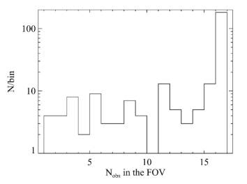
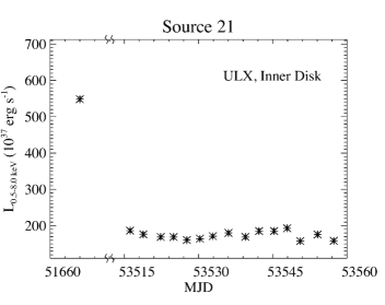
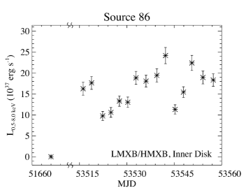
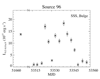
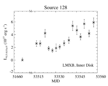
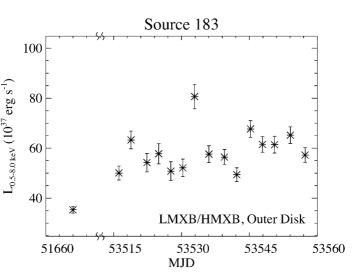
We consider sources with $S_{\mathrm{flux}}>3$ to have significant variability. For sources that are in the field of view of all observations (see Fig. 6), we find that 16% of them exhibit significant variability on the days–weeks timescales and 25% of the sources exhibit significant variability on the 5-year timescale. For some sources, we find considerable variability as much as approximately an order of magnitude in luminosity. However, we likely have missed substantial variations in some sources, especially some of the fainter ones, because of limited signal-to-noise and how we search for variability. Thus, the fraction of the population that we measure as variable is a lower limit.

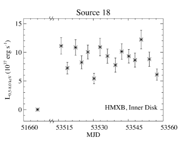
We plot light curves of the 6 sources with the strongest variability in either of the two different timescales ($S_{\mathrm{flux}}>11$; Fig. 7). In these 6 most extreme cases, the most significant variability always occurs on the 5-year timescale (at least in part due to the smaller errors in the luminosities associated with this timescale comparison). In addition, all of these sources have colors in Fig. 5 consistent with LMXBs and HMXBs ((H-M)/T$=-0.5$–0.0 and (M-S)/T = 0.0–0.5) except for source number 96, which is consistent with a SSS.

For the remainder of the variable sources, we see a wide range in the level and timescale of variability. However, there appear to be groups of sources with similar variability characteristics. For instance, there is a group of sources ($\sim 20$) that have luminosities on the order of a few times 10³⁶ erg s^-1 or less for most of the observations, but that brighten by about an order of magnitude over 1-3 observations or a timescale of a few days. In particular, six of these sources, which all have colors consistent with HMXBs, brighten by a factor of 5–30 over one of ObsIDs 5935-5949 ($\sim 2.5\sigma$). One of these sources is in the outer disk region and five are in the inner disk region. Sources undergoing an outburst like these could be population of massive star transient sources (e.g., Be star binaries) like those in the Magellanic Clouds and our Galaxy (e.g., Liu et al., 2006; Meurs & van den Heuvel, 1989).

5.2. Spectral Variability

We also tested for spectral variability by constructing the same variability statistic as in equation (1) for the column density and power-law index or blackbody temperature. The fluxes in this equation are replaced by the best-fit values of these parameters and the flux uncertainties are replaced by the uncertainties from the spectral fits.

In the master source list, significant spectral variability based on the column density was found for only one source, number 21 (the brightest source and ULX). The variability was found only for the comparison of the merged observation and ObsID 735 for the 5-year timescale. Significant spectral variability based on the power-law index was found for only four sources: 5, 6, 19, 22. The most significant variability for sources 5 and 22 occurs on the days–weeks timescale and, for sources 6 and 19, occurs on the 5-year timescale between single observations. There were no sources with significant variability in the blackbody temperature.

All of these sources have colors consistent with LMXBs and HMXBs ((H-M)/T$=-0.4$–0.0 and (M-S)/T = 0.1–0.6). Detecting significant spectral variability in only a few cases is not unexpected given the very low signal-to-noise ratio for most sources in the individual observations. Finally, as was the case for the flux variability, we note that the amount of spectral variability only represents a lower limit to the spectral variability.

6. Luminosity Functions

Table 3Lower Luminosity Cutoffs for the XLF Comparisons

Comparison	Luminosity Cutoff ($10^{37}$ erg s-1)
Type	Entire Galaxy	Bulge	Inner Disk	Outer Disk
ObsIDs 5935–5949 (days–weeks)	2.9	1.3	2.6	2.9
ObsIDs 5935–5949 to 735 (5-year)	5.1	1.7	5.1	3.8
Merged to ObsID 735 (5-year)	1.8	0.33	1.5	1.3
ObsIDs 5935–5949 to Merged	1.5	0.80	1.5	1.5

Note. — We include the comparison of the merged to ObsID 735 XLF because it goes considerably deeper.

Figure 8.— Example cumulative XLFs for ObsID 5948 for sources that are in the field of view of all 16 observations. Each plot represents a different region of M81.

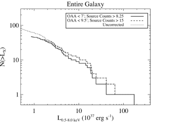
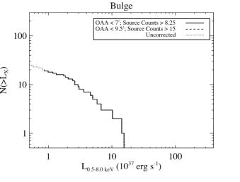
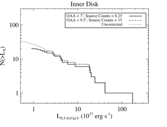
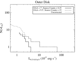
We construct XLFs of each region of the galaxy (all regions, bulge, inner disk, and outer disk; see § 4) for each observation (ObsIDs: 5935–5949, 735; Fig. 8) and for the merged observation (Fig. 11). Because of non-uniform coverage in the disk fields and because we test for variability from observation to observation, we carefully selected sources in the field of view of all 16 observations (see Figs. 1 and 6). As noted in § 4, we do not remove contaminating foreground/background sources in our fields on a source-by-source basis, since we cannot differentiate such sources based on the X-ray observations alone. We only make a global correction to the XLFs for the expected AGN luminosity function, which we detail below. Detailed source matching, which will be completed in a future publication, will help to mitigate the contamination of foreground/background sources and enable us to separate populations of sources in more detail (Zezas et al. in prep.).

6.1. Incompleteness Correction

The source detection threshold is not consistent over the entire field of view of each of the observations or the merged observation because of a variety of instrumental and statistical effects (e.g., varying PSF size and shape, effective detector area, etc.). This leads us to detect only a fraction of sources at lower luminosities, and, as a result, any XLF that we construct near the detection threshold of our observations will be shallower due to incompleteness. Therefore, we correct all of our XLFs for incompleteness using the methods in Zezas et al. (2007) before any comparisons and fits are attempted.

In brief, the detection probability of a source is calculated for multiple background levels and off-axis angles from grids of MARX simulations (Wise et al., 2003). Then, on a source-by-source basis, we interpolate between these grids to estimate the detection probability and, hence, the incompleteness correction factor to be applied to each source in each XLF.

We apply incompleteness corrections for each XLF based on one of two sets of cutoffs, each set having two cutoffs: a source count cutoff and an off-axis angle cutoff. A source count cutoff is important because we do not correct for Eddington bias (Eddington, 1913) and an off-axis angle cutoff is important because the detection threshold grows considerably toward large off-axis angles. Each source must to have either more than 8.25 source counts and an off-axis angle less than 7 arcminutes or more than 15 source counts and an off-axis angle less than 9.5 arcminutes, depending on which region of the galaxy it resides. Beyond 9.5 arcminutes, the incompleteness correction for almost any luminosity included in our source list is exceedingly large. At count cutoffs greater than 15 counts, we reject too many sources to construct useful XLFs.

For all of the XLF comparisons and fitting, we always used the largest off-axis angle cutoff for the entire galaxy, inner disk, and outer disk regions, and the smaller off-axis angle cutoff for the bulge. We took care to uniformly impose our off-axis angle and count limits across all observations, so that if a source fails to meet our criteria in one observation, the same source was rejected in all other observations. This is very important so that when we compare our XLFs, any differences in the XLFs are from source variability alone, not source rejection. Finally, for the XLF tests for variability in the next section, we only compared the XLFs above certain luminosities where the completeness of the XLFs is greater than $\sim 20\%$ (Table 3).

6.2. Testing for XLF Variability

A large percentage of the individual sources included in the XLFs exhibit variability: 58% (entire galaxy), 36% (bulge), 60% (inner disk), 43% (outer disk). Can this individual source variability impart significant varibility to the XLFs? We directly test this hypothesis.

When comparing our corrected XLFs, we used a non-parametric statistical test, the Kolmogorov-Smirnov (K-S) test (Kolmogorov, 1941). We also arrived at the same conclusions as below for the K-S test when testing the uncorrected XLFs with the Kruskall-Wallis (K-W) (Kruskal, 1952) and Mann-Whitney (M-W) tests (Mann & Whitney, 1947). Helpful detailed explanations of these and other similar statistical tests can be found in Siegel (1956).

The K-S test is useful because it could be applied to the incompleteness-corrected XLFs. We tested our XLFs for consistency by making pairwise comparisons of the XLFs using a two-sided K-S test, which indicates how likely it is that the two XLFs were drawn from the same parent distribution. A K-S statistic near 0 indicates that two data sets were not drawn from the same parent distribution.

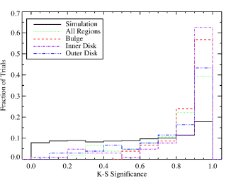
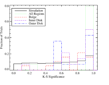
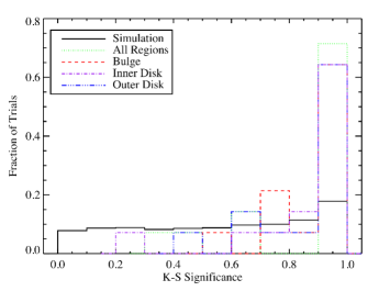
To test the XLFs for consistency, we considered two different timescale comparisons separately, a timescale of days–weeks (ObsIDs 5935–5949) and a timescale of $\sim 5$ years (ObsIDs 5935–5949 to 735 and merged to ObsID 735). In doing so, we also compared the XLFs in each of our different fields of view separately (entire galaxy, bulge, inner disk and outer disk regions). In addition, we test for the possibility that differences in the merged and individual XLFs arise because of differences in individual source luminosities in a snapshot versus the average luminosity (see section 4.1 of Zezas et al., 2007). Upon inspecting the distributions of these K-S significance statistics (Figs. 9 and 10), we find that, although most of the K-S statistics are near 1 for all regions of the galaxy, some of them are near 0.

To explore the possible significance of this, we randomly generated 10000 XLFs by drawing 100 sources from a power-law distribution with index $-1.5$ (the exact number of sources and slope does not matter). Then, we performed the same pairwise K-S analysis on the generated XLFs and plotted the distribution of K-S statistics (Figs. 9 and 10). Thi Monte Carlo simulation shows that having a non-neglible number of K-S values near 0 is expected for random samples drawn from the same parent distribution. Futhermore, from the comparison of the merged XLF to the ObsID 735 XLF, we found KS statistics: 0.98 (entire galaxy), 0.76 (bulge), 0.99 (inner disk) and 0.91 (outer disk). Therefore, we conclude that the observed M81 XLFs for either timescale are consistent with being drawn from the same distribution. The intrinsic variability of the individual M81 sources on these timescales does not make the XLFs inconsistent with each other, suggesting that a snapshot survey provides a reliable indicator of the XLF.

6.3. XLF Fitting

Figure 9.— The measured and simulated distribution of the K-S statistics between ObsIDs 5935–5949 (days–weeks timescale; left) and of ObsIDs 5935–5949 to ObsID 735 (5-year timescale; right). The measured distributions are constructed from XLFs from sources in the field of view of all observations included in the comparison, taking into account the off-axis angle, count, and completeness thresholds discussed in § 6.1 and § 6.2.

Figure 10.— The measured and simulated distribution of the K-S statistics for comparing each of the individual ObsIDs 5935–5949 to their merged observation. The measured distributions are constructed from XLFs from sources in the field of view of all observations included in the comparison, taking into account the off-axis angle, count, and completeness thresholds discussed in § 6.1 and § 6.2.

Figure 11.— Merged cumulative XLFs for sources that are in the field of view of the merged ObsIDs. Each plot represents a different region. The best-fit power-law models are plotted as listed in Table 4 (see § 6.3). We compare our entire galaxy XLF to the total disk XLF of M31 (Shaw Greening et al., 2009) by normalizing it to the M81 models at $10^{37}$ erg s^-1 and plotting it as dim dash-dotted line on our entire galaxy XLF. We also compare our bulge XLF to the LMXBs for the Milky Way (Grimm et al., 2002) and the inner $17^{\prime}\times 17^{\prime}$ (bulge) of M31 (the cutoff power-law model Kong et al., 2003) as above. Note that all of these studies use different energy ranges and methods for calculating the luminosities, which contributes to systematic differences in the XLFs that are not accounted for here. Also, the XLF fits are affected by the contribution of AGN to varying degrees, depending on the region of the galaxy considered. The expected contribution of AGN to the low-luminosity end of the XLFs, in particular, appears to be too large for the M81 field. The correction for AGN and its limitations are discussed in more detail in § 6.3.

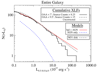
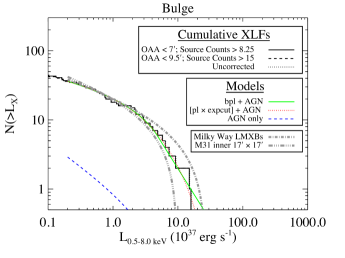
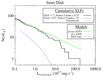
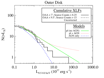
Parameterizing the XLFs is useful for comparing our XLFs to XLFs in other galaxies and those created by synthesis models. Therefore, we fit the differential XLFs with simple and modified power-law functions. There are a number of methods that can be used to fit a differential number of points in an unbiased way: maximum likelihood methods (Clauset et al. 2007, Zezas et al. 2007), a method using the K-S test (Johnston & Verbunt, 1996), or methods using X-ray spectral fitting software (Kenter & Murray 2003, Zezas et al. 2007).

6.3.1 Our XLF Fitting Method and Models

We choose to use the method utilizing X-ray spectral fitting software because it is convenient and has been shown to yield consistent results with a maximum likelihood method (see Zezas et al., 2007). Furthermore, we can implement the incompleteness correction through an ARF that scales the differential number of sources for the fitting.

Because of our large dynamic range for fitting ($2\times 10^{36}$–$2\times 10^{39}$ erg s^-1), we rebin the XLF and ARF in counts space to six-count bins as opposed to a “natural” binning scheme of one-count bins. This prevents the ARFs from becoming too large, which results in the fits taking a very long time to run or Sherpa crashing. Over a smaller dynamic range, we verified that the best-fit parameters do not change significantly when we use this variation of the “natural” binning scheme.

Both the ARF and XLF are read into Sherpa 3.4 and fit just like a typical X-ray spectrum with the C-Statistic since the number of counts in each bin are very small. We first tried fitting the differential merged XLFs for each of the four regions (entire galaxy, bulge, inner disk, outer disk) with a single power law of the form:

$$\frac{dN}{dL}=A\left(\frac{L}{L_{ref}}\right)^{-\alpha_{1}}$$ (2)

where the reference luminosity, L${}_{\text{ref}}$, is always set to $10^{37}$ erg s^-1 and A is the amplitude at the reference luminosity (cumulative slope = $\alpha_{1}-1$). We also considered a broken power law of the form:

$$\frac{dN}{dL}=\left\{\begin{matrix}A\left(\dfrac{L}{L_{b}}\right)^{-\alpha_{1}}\quad\text{for}\ L\leq L_{b}\\ A\left(\dfrac{L}{L_{b}}\right)^{-\alpha_{2}}\quad\text{for}\ L\geq L_{b}\end{matrix}\right.$$ (3)

so that the amplitudes and reference luminosities of the two power laws match and the reference luminosity is defined as the break luminosity, L_b. In addition, given that the bulge XLF appears truncated, we also fit a power law with an exponential cutoff to it of the form:

$$\frac{dN}{dL}=A\left(\frac{L}{L_{ref}}\right)^{-\alpha_{1}}e^{C(L-L_{b})}$$ (4)

where C is a constant and L_b is the offset or break luminosity.

Lastly, AGN number counts (Rosati et al. 2002, Bauer et al. 2004, and Kim et al. 2007) suggest that background AGN make up a non-negligible fraction of the sources in our XLFs. We attempt to compensate for the AGN contribution in our model fits by adding a fixed flux distribution of AGN to all of the models in equations (2)–(4) before fitting. As is clear from work on the number counts of AGN mentioned above, we can describe the distribution by a broken power law with differential indices $\sim 1.6$ and 2.5 (Euclidean) below and above the break. We use the broken power-law model (different in functional form to ours above) and fit parameters exactly as given in the number count results of the CHAMP survey (see equations (3)-(5) and Table 3 of Kim et al., 2007). We use the row of parameters in Table 3 of Kim et al. 2007 derived using a photon index of 1.7 and that match our energy range (0.5–8.0 keV).

We report all of our fit results excluding and including the AGN contribution in Table 4.

Table 4Merged XLF Fits

	Without the AGN Model				With the AGN Model
	$\alpha_{1}$	$\alpha_{2}$ or	Amplitude†	Lb	$\alpha_{1}$	$\alpha_{2}$ or	Amplitude†	Lb
Region (Model)		Coeff.‡		($10^{37}$ erg s-1)		Coeff.‡		($10^{37}$ erg s-1)
All	1.00${{}_{-0.19}^{+0.12}}$	1.67${{}_{-0.08}^{+0.10}}$	29.43${{}_{-3.44}^{+3.32}}$	1.21${{}_{-0.09}^{+0.23}}$	0.26${{}_{-0.60}^{+0.35}}$	1.60${{}_{-0.08}^{+0.12}}$	21.49${{}_{-3.36}^{+4.50}}$	1.20${{}_{-0.22}^{+0.14}}$
Bulge (bpl)	1.06${{}_{-0.18}^{+0.09}}$	2.49${{}_{-0.40}^{+0.54}}$	1.77${{}_{-0.44}^{+0.32}}$	4.87${{}_{\mathrm{NA}}^{\mathrm{NA}}}$	1.01${{}_{-0.20}^{+0.11}}$	2.50${{}_{-0.41}^{+0.56}}$	1.75${{}_{-0.45}^{+0.35}}$	4.87${{}_{\mathrm{NA}}^{\mathrm{NA}}}$
Bulge (pl $\times$ expcut)	0.92${{}_{-0.25}^{+0.23}}$	-0.12${{}_{-0.08}^{+0.06}}$	4.20${{}_{-3.80}^{\mathrm{NA}}}$	8.00${{}_{\mathrm{NA}}^{\mathrm{NA}}}$	0.86${{}_{-0.27}^{+0.25}}$	-0.13${{}_{-0.08}^{+0.06}}$	2.87${{}_{-2.82}^{\mathrm{NA}}}$	9.90${{}_{\mathrm{NA}}^{\mathrm{NA}}}$
Inner Disk	1.44${{}_{-0.08}^{+0.09}}$	NA	11.91${{}_{-1.59}^{+1.75}}$	NA	1.31${{}_{-0.11}^{+0.11}}$	NA	7.21${{}_{-1.68}^{+1.82}}$	NA
Outer Disk	1.58${{}_{-0.12}^{+0.13}}$	NA	6.99${{}_{-1.22}^{+1.38}}$	NA	1.16${{}_{-1.07}^{+0.37}}$	NA	0.76${{}_{-0.84}^{+1.32}}$	NA

Note. — Best XLF model fit parameters as defined in equations (2)–(4) with and without the background AGN broken power-law model contribution (based on AGN number counts). We fit and report the fit information for the differential XLFs. All of the XLFs were fit over the range $2\times 10^{36}$–$2\times 10^{39}$ erg s^-1, where the completeness is greater than $\sim 50\%$. The slopes are systematically shallower with the AGN model included and shallower than expected compared to XLF slopes of similar galaxies. This suggests that the expected contribution of AGN to the low-luminosity end of the XLFs, in particular, could be too large for the M81 field. See § 6.3 for model definitions and further background AGN discussion. In various places throughout the table, NA = “Not Applicable/Available” is used because there is either no slope, coefficient, or break luminosity for a straight powerlaw or because the Sherpa uncertainty estimates did not converge.

($\dagger$) The power-law reference points for the amplitude (number of sources at the reference luminosity in the differential XLF) are always equal to $10^{37}$ erg s^-1 for the single power-law model or the exponential cutoff model for the bulge and equal to the break luminosity for the broken power-law model.

($\ddagger$) In the case of the bulge power law with an exponential cutoff, the exponential coefficient, “C”, as in equation (4).

6.3.2 Discussion of XLF Fit Results by Region

First, the contribution from AGN is a serious issue in most of our fields. The AGN contribution increases at smaller fluxes because it appears that the LogN–LogS slope is steeper than the slope of the M81 XLF. At face value, including the AGN distribution forces the best-fit power-law slopes for M81 to be shallower in all of the XLFs. However, foreground absorption of M81 brings about an uncertainty in the AGN flux distribution. The foreground absorption is difficult to quantify because the clumpiness of the disk suggests a highly variable column density. A disk scale height of a few hundred parsecs for a typical ISM density of $\sim 1$ cm^-3 at the inclination of M81 ($\sim 35^{\circ}$; Boggess, 1959) produces an average column density $\sim 10^{21}$ cm^-2 measured perpendicular to the disk. This could decrease the flux of a typical AGN by $\sim 10\%$, flattening the faint-end slope of logN–LogS for AGN in this region.

The uncertainty from foreground absorption together with galactic foreground diffuse emission from M81, standard errors in the survey measurements, and cosmic variance make interpreting our XLFs very difficult, especially at the faint ends. For example, an uncertainty of $\sim 20\%$ due to cosmic variance and an equally sizable shift brought about by the foreground emission and absorption of M81 changes the best-fit slope of the outer disk by $\sim 0.1$ and the amplitude by $\sim 70\%$. Note that the AGN contamination varies with the galactic source density (see Table 4 and Figure 11) so that the bulge XLF is least affected and the outer disk XLF is most affected. In light of these complications, we are still able to make some concrete statements regarding our XLFs.

In order to interpret our XLF fits, we need to compare the significance of the fits between the single and broken power-law models. Since the C-Statistic, a maximum likelihood statistic, is used, it is appropriate to compare the quality of the fits using a likelihood ratio test (e.g., Zezas et al., 2007). We simulate 1000 XLFs from a single power-law model and then fit them with the single and the broken power-law model in the same way that we fit the observed XLFs. We then calculate the ratio of the single to the broken power-law best-fit C-statistics for each XLF. The confidence level corresponding to the amount of improvement of the fit from the single to the broken power-law model is the fraction of times that the simulated ratio of statistics is greater than the measured ratio of the statistics. One should not judge the quality of the fits from the best-fit cumulative distribution functions on the logarithmically-scaled plots because they can be misleading. For instance, uncertainties in the XLFs at the high-luminosity end are much larger than those at the low-lumionsity end. In addition, unexpected statistical effects frequently caused by the skewness in the probability distribution of sources comprising the XLFs have been documented previously (Gilfanov et al. 2004; Clauset et al. 2007).

In the bulge, we find that the broken power-law model and the power-law model with an exponential cutoff provide a highly-significant improvement in the fit versus a single power law ($>99.9\%$ confidence, $\gg 3\sigma$). The break luminosity is poorly constrained but is within a factor of a few of the Eddington luminosity of a neutron star and is consistent with the values derived from other previous work for elliptical and S0 galaxies, the bulges of other galaxies, and the LMXBs of our Galaxy (Sarazin et al., 2000; Blanton et al., 2001; Kundu et al., 2002; Grimm et al., 2002; Kim et al., 2006; Voss et al., 2009). We also see evidence of the flattening of the LMXB XLF below $\sim 10^{37}$ erg s^-1 that has been seen by many of these previous studies. The best fit functions with the AGN model are

$$\frac{dN}{dL}=\left\{\begin{matrix}1.75\left(\dfrac{L}{L_{b}}\right)^{-1.01}\quad\text{for}\ L\leq L_{b}\\ 1.75\left(\dfrac{L}{L_{b}}\right)^{-2.50}\quad\text{for}\ L\geq L_{b}\end{matrix}\right.$$ (5)

for the broken power law, where L${}_{\text{b}}=4.87\times 10^{37}~{}\mathrm{erg~{}s}^{-1}$ and

$$\frac{dN}{dL}=2.87\left(\frac{L}{10^{37}\,{\rm erg\,s^{-1}}}\right)^{-0.86}e^{-0.13\left(L-L_{b}\right)}$$ (6)

for the power law with an exponential cutoff, where L${}_{\text{b}}=9.9\times 10^{37}~{}\mathrm{erg~{}s}^{-1}$.

The shape of this XLF together with the locations of the sources in the color-color plot (Fig. 5) suggests a very old population of stars dominates the innermost part of M81 and that we are probing a population of mostly LMXBs. The shape of the XLF is also consistent with the overall shape of the average LMXB XLF, which has a flat cumulative distribution below a few times $10^{37}$ erg s^-1 with a cutoff near a few times $10^{38}$ erg s^-1 (Gilfanov, 2004). The AGN do not strongly bias these results as they are expected to comprise $\lesssim 10\%$ of the sources in the XLF above the cutoff luminosity, $2\times 10^{36}$ erg s^-1.

Next, because of the very large percentage of AGN expected in the outer disk XLF ($\sim 80\%$ of the sources above the cutoff luminosity and $\sim 60\%$ of the sources above $10^{37}$ erg s^-1), this region is the most difficult to interpret. This region also has the fewest total number of sources, and brief inspection of some all-sky optical surveys suggests that there are also a few foreground stars, which we have not attempted to remove. While there appears to be a break near $10^{37}$ erg s^-1, it does not bring about a significant improvement in the fit when the AGN contribution is taken into account (94% confidence, $1.9\sigma$).

Therefore, we fit this XLF with a single, unbroken power law as is typically seen in disk-like regions of ongoing star formation as in the disk XLF of our Galaxy (Grimm et al., 2002), the Antennae (Zezas et al., 2007), and NGC 6946 (Fridriksson et al., 2008), for examples. The best-fit function with the AGN model is

$$\frac{dN}{dL}=0.76\left(\frac{L}{10^{37}~{}\mathrm{erg~{}s}^{-1}}\right)^{-1.16}$$ (7)

with a much shallower slope than what has been found in the studies above and which produces an unusual-looking fit (Fig. 11). However, the best-fit function without the AGN model is

$$\frac{dN}{dL}=6.99\left(\frac{L}{10^{37}~{}\mathrm{erg~{}s}^{-1}}\right)^{-1.58}$$ (8)

with a slope that is more consistent with the other disk studies above. The slope cannot be well-constrained and, given the large fit uncertainties (the errors for the slopes are on the order of the range of slopes found with or without the AGN model), we do not attempt to interpret this XLF further.

Our inner disk region XLF is consistent with a single, unbroken power law and a broken power law does not result in a significant improvement in the fit (44% confidence, $<1\sigma$). The best-fit function with the AGN model is

$$\frac{dN}{dL}=7.21\left(\frac{L}{10^{37}~{}\mathrm{erg~{}s}^{-1}}\right)^{-1.31}$$ (9)

Inspection of the color-color plot (Fig. 5) indicates that there are a population of LMXBs in this region (or HMXBs with black holes that have very similar colors) that are embedded with the HMXBs and other sources (this is also where the ULXs and a few SNRs are). While visual inspection of Figure 11 may suggest that this XLF has a break, the fits indicate that it is not significant. Furthermore, the best-fit power-law slope and the fact that well-pronounced spiral arms are present, combined with an inspection of Fig. 5, supports the notion that this XLF appears very disk-like and that a large fraction of the sources in this region are HMXBs. The AGN make a moderate contribution to the sources in the XLF here ($\sim 30\%$ of the sources above the cutoff luminosity) and do change the slope and normalization of the best-fit model when taken into account. However, whether we take into account the AGN contribution or not, a single power law is strongly favored and the best-fit slopes in either case are consistent with each other.

A global view of X-ray point source population is revealed in the total XLF. There is a marginal improvement in the fit from the single to the broken power law (97% confidence, $2.2\sigma$) with a break near $10^{37}$ erg s^-1, which could be the break in the bulge manifesting itself at a slightly lower luminosity than measured in the bulge. The best-fit function with the AGN model is

$$\frac{dN}{dL}=\left\{\begin{matrix}21.49\left(\dfrac{L}{L_{b}}\right)^{-0.26}\quad\text{for}\ L\leq L_{b}\\ 21.49\left(\dfrac{L}{L_{b}}\right)^{-1.60}\quad\text{for}\ L\geq L_{b}\end{matrix}\right.$$ (10)

where L${}_{\text{b}}=1.20\times 10^{37}~{}\mathrm{erg~{}s}^{-1}$ and without the AGN model is

$$\frac{dN}{dL}=\left\{\begin{matrix}29.43\left(\dfrac{L}{L_{b}}\right)^{-1.00}\quad\text{for}\ L\leq L_{b}\\ 29.43\left(\dfrac{L}{L_{b}}\right)^{-1.67}\quad\text{for}\ L\geq L_{b}\end{matrix}\right.$$ (11)

where L${}_{\text{b}}=1.20\times 10^{37}~{}\mathrm{erg~{}s}^{-1}$. The slopes with or without the AGN model are fairly shallow and resemble the XLF slope of the inner disk region of M81 and disk regions in other galaxies where there is considerable star formation occurring. However, because this XLF does also have a significant break and the color-color plot (Fig. 5) suggests contributions from many different populations of sources, we conclude that this XLF is neither disk- nor bulge-dominated, but is a fairly even mixture of both types.

Finally, we can use our XLFs to estimate two interesting galactic properties: the stellar mass and the SFR, using relationships in Gilfanov (2004) and Grimm et al. (2003), respectively.

First, to estimate the total stellar mass of M81, we need to estimate the number of LMXBs in M81 with L${}_{\text{X}}>10^{37}$ erg s^-1. Since we have found that the bulge is likely almost exclusively composed of LMXBs, we use our bulge XLF to estimate that there are $\sim 20$ LMXBs in this range. As we have stated above, we also expect there to be a population of LMXBs in the disk regions as well, especially in the inner disk region. The fraction of LMXBs can be estimated from our color-color plot (Fig. 5) but is very uncertain. Taking this fraction and applying it to our XLF in this luminosity range, we estimate that there are $\sim 10$ LMXBs in this region. The outer disk region appears to contribute only a very small amount of LMXBs with L${}_{\text{X}}>10^{37}$ erg s^-1 when the expected AGN fraction is taken into account, so we do not include it here.

Then using these numbers together with equation 20 in Gilfanov (2004), we estimate that the total stellar mass of M81 is $>2.1\times 10^{10}$ M_☉. This is a fairly robust lower limit to the number LMXBs in M81 because: we have neglected the outer disk contribution, the K-band light is measured out to larger radii than our X-ray data, there are some sources superimposed against the LINER nucleus that we are unable to detect or classify (some of these are the ML sources in Table 2), and equation 21 suggests a larger mass.

We also estimate the total stellar mass of M81 using the total 2MASS K-band magnitude, $\sim 3.9$ mag. This corresponds to a solar K-band luminosity of $7.7\times 10^{10}$ L_☉. Using M_∗/L${}_{\text{K}}\approx 1.1$ from GALEV models for an SAab-type galaxy (Kotulla et al., 2009), we estimate a total stellar mass of $8.5\times 10^{10}$ M_☉. Reversing the calculation, this stellar mass suggests that M81 has $\sim 70$–120 LMXBs with L${}_{\text{X}}>10^{37}$ erg s^-1. Part of this discrepancy can be attributed to the reasons listed at the end of the previous paragraph. Other reasons include uncertainties in the M_∗/L${}_{\text{K}}$ ratio of M81 and of the values assumed by Gilfanov (2004), which, together, could contribute deviations of factors of approximately two to three. For these reasons, caution should be taken in estimating the number of LMXBs and stellar mass using this method for M81 and other galaxies with similar issues.

Second, to estimate the SFR, we need to estimate the total number of HMXBs and their total luminosity for L${}_{\text{2--10 keV}}>2\times 10^{38}$ erg s^-1. There are four sources with L${}_{\text{2--10 keV}}>2\times 10^{38}$ erg s^-1. Inspection of the locations of these sources in Fig. 5 suggests that at least one of these sources is likely to be a HMXB. The other three sources all lie on the boundary between HMXBs and LMXBs. This, combined with the knowledge that the color of an individual source is not sufficient to determine the precise nature of the source (§ 4), and the fact that we are subject to large Poisson errors at the high-luminosity end of the XLF, only allows us to place approximate limits on the SFR estimated with this method. Equation 20 of Grimm et al. (2003) suggests a range of SFRs of 0.34–1.38 M_☉ yr^-1 for 1–4 sources with L${}_{\text{2--10 keV}}>2\times 10^{38}$ erg s^-1, and equation 22 of Grimm et al. (2003) suggests a range of SFRs of 0.52–1.02 M_☉ yr^-1 for the range of luminosities of these sources, 1.34–$2.64\times 10^{39}$ erg s^-1. These estimates are comparable to the SFR that has been estimated for M81 based on a combination of ultraviolet, H$\alpha$, and infrared observations (0.3–0.9 M_☉ yr^-1; e.g., Gordon et al., 2004).

7. Comparing the XLFs of M81 with Those of Two Other Nearby Similar Spiral Galaxies

M81, M31, and our Milky Way are all Sb-type galaxies with similar SFRs near 1 M_☉ yr^-1. Below, we make comparisons of the global properties of their X-ray binary populations using their XLFs.

7.1. Comparisons With the Milky Way

First, the XLFs of both the inner and outer disk regions of M81 are systematically shallower than the HMXB slope of the Milky Way, but, given the statistical uncertainties and uncertainties in the AGN contribution, are fairly consistent with one another. While the M81 inner and outer disk regions do appear to be dominated by HMXBs, they also contain other types of sources (e.g., AGN, SNRs) that we are unable to separate conclusively on an individual basis at the present time.

Second, the near match of the M81 bulge and the normalized LMXB population in the Milky Way is striking (Fig. 11). We find that the low-luminosity LMXB slope of the Milky Way is similar to the low-luminosity slope found for the M81 bulge within the uncertainties. Also, the cutoffs in the LMXB XLFs are within a factor of $\sim 2$ of one another, supporting the notion that the bulge of M81 is dominated by LMXBs as seen in the color-color plot (Fig. 5).

7.2. Comparisons With M31

We find that the normalized XLF of the inner $17^{\prime}\times 17^{\prime}$ region of M31 as measured with Chandra by Kong et al. (2003) is quite similar to the bulge XLF of M81 (Fig. 11). These data also match well to the bulge region observations measured with XMM-Newton (r$<15^{\prime}$) by Trudolyubov et al. (2002).

The disk XLFs of M31 are more difficult to compare as studies of the M31 disk return different results (Kong et al. 2003, Shaw Greening et al. 2009). Although the XLFs in each of the disk regions are consistent with single, unbroken power law, as expected, the power-law slopes measured by each group are significantly different. We examine some of the reasons for these differences below.

The disk XLFs of Kong et al. (2003) do not include ULXs or any sources brighter than $\sim 3\times 10^{37}$ erg s^-1 (unlike the disk XLFs in M81 and the HMXB XLF of the Milky Way). However, the field of view of Chandra is much smaller than M31 and all of the Chandra fields in Kong et al. (2003) together still only cover a fraction of the disk of M31. As noted in Shaw Greening et al. (2009), there are much brighter sources seen in their fields, which cover most of the M31 disk that are being missed in small-area surveys. Missing these brighter sources could truncate the high-luminosity end of Kong et al. (2003)’s disk XLFs, and could make these XLFs steeper. However, the effect that a few bright sources have on the best-fit slope is not obvious without further detailed analysis, which is beyond the scope of this paper.

Second, (as pointed out in Shaw Greening et al., 2009, see their Figure 5), model bias in the spectral fitting of each of the point sources that comprise the XLF could affect the best-fit normalization and slope of the XLF. For instance, Kong et al. (2003) fit all of their sources with a fixed, absorbed power law, which could be biasing their XLFs. We could also be slightly biased by choosing a power law as our initial fitting model, but we expect this to have a smaller effect because we have allowed for the possibility of a model that better describes softer sources (blackbody). In addition, we float our photon index or blackbody temperature for all sources with more than 25 counts and always float our column densities for all sources with more than 5 counts.

Thoroughly assessing the impact of a single versus a variable conversion factor on the XLFs directly is beyond the scope of this paper. However, we can make some simple statistical comparisons for the merged luminosities of the sources in the master source list. We compare the error that would arise from using a single conversion factor to calculate the luminosities (Fig. 3) and the statistical error in the luminosity scaled from the Bayesian error in the counts. We find that the shape of both distributions is very similar, but that the median and the width of the distribution of the statistical percent error is greater than the median (by approximately a factor of 1.5) and the width of the distribution of the percent error that would arise from using a single conversion factor. Because the conversion factor errors are typically smaller than the statistical errors in the luminosity, we suspect that the effect on the XLFs would probably be fairly small, but maybe non-negligible.

In light of these issues, we only compare our disk and entire galaxy XLF results to the disk XLFs constructed by Shaw Greening et al. (2009). The total disk XLF that these authors construct surprisingly seems to better match the M81 XLF of the entire galaxy rather than the inner or outer disk XLFs. First, they claim a break in their total disk XLF, which happens to coincide with the measured break in the M81 XLF of the entire galaxy. Also, the power-law slopes are in good agreement with the slopes that we measure for M81’s entire galaxy XLF. These results suggest that the disk of M31 has a high-luminosity component similar to what is seen in the inner and outer disks of M81, but it also seems to have a more considerable population of LMXBs there that produce at least a marginally significant break near $10^{37}$ erg s^-1.

8. Summary

We have presented an in-depth analysis of multiple aspects of the X-ray source population of M81 from the perspective of the X-ray observations alone. We conducted our source detection procedure carefully, producing a master source list of 265 sources. We then extracted and individually fit the spectra for each of these sources in each of the 16 observations of M81 included in our analysis. With the spectral information, we calculated hardness ratios and used the aid of a color-color plot to classify different populations of sources. From the population study, we devised an alternate conservative method of separating the bulge and the disk of the galaxy. Then, we quantified the variability of the individual sources and considered their possible effect on the luminosity function of the galaxy. We find that, despite detecting significant variability in $\sim 36$–60% of the sources included in the XLFs, the XLF of M81 remains stable at luminosities greater than $\sim 2\times 10^{37}$ erg s^-1. Finally, we plotted and fit the XLFs, analyzed them with regard to their point source populations, and compared them to the XLFs of M31 and the Milky Way.

References

- Angelini et al. (2001) Angelini, L., Loewenstein, M., & Mushotzky, R. F. 2001, ApJ, 557, L35
- Bauer et al. (2004) Bauer, F. E., Alexander, D. M., Brandt, W. N., Schneider, D. P., Treister, E., Hornschemeier, A. E., & Garmire, G. P. 2004, AJ, 128, 2048
- Belczynski et al. (2008) Belczynski, K., Kalogera, V., Rasio, F. A., Taam, R. E., Zezas, A., Bulik, T., Maccarone, T. J., & Ivanova, N. 2008, ApJS, 174, 223
- Blanton et al. (2001) Blanton, E. L., Sarazin, C. L., & Irwin, J. A. 2001, ApJ, 552, 106
- Boggess (1959) Boggess, N. W. 1959, PASP, 71, 534
- Broos et al. (2010) Broos, P. S., Townsley, L. K., Feigelson, E. D., Getman, K. V., Bauer, F. E., & Garmire, G. P. 2010, ApJ, 714, 1582
- Cash (1979) Cash, W. 1979, ApJ, 228, 939
- Clauset et al. (2007) Clauset, A., Rohilla Shalizi, C., & Newman, M. E. J. 2007, ArXiv e-prints
- Colbert et al. (2004) Colbert, E. J. M., Heckman, T. M., Ptak, A. F., Strickland, D. K., & Weaver, K. A. 2004, ApJ, 602, 231
- Davis (2001) Davis, J. E. 2001, ApJ, 562, 575
- Dickey & Lockman (1990) Dickey, J. M., & Lockman, F. J. 1990, ARA&A, 28, 215
- Eddington (1913) Eddington, A. S. 1913, MNRAS, 73, 359
- Fabbiano (1988) Fabbiano, G. 1988, ApJ, 325, 544
- Fabbiano & White (2006) Fabbiano, G., & White, N. E. 2006, in Compact stellar X-ray sources, ed. Lewin, W. H. G. & van der Klis, M. (University of Chicago Press), 475–506
- Fabbiano et al. (2010) Fabbiano, G., et al. 2010, ApJ, 725, 1824
- Fragos et al. (2008) Fragos, T., et al. 2008, ApJ, 683, 346
- Freedman et al. (1994) Freedman, W. L., et al. 1994, ApJ, 427, 628
- Freeman et al. (2001) Freeman, P., Doe, S., & Siemiginowska, A. 2001, in Society of Photo-Optical Instrumentation Engineers (SPIE) Conference Series, Vol. 4477, Society of Photo-Optical Instrumentation Engineers (SPIE) Conference Series, ed. J.-L. Starck & F. D. Murtagh, 76–87
- Freeman et al. (2002) Freeman, P. E., Kashyap, V., Rosner, R., & Lamb, D. Q. 2002, ApJS, 138, 185
- Fridriksson et al. (2008) Fridriksson, J. K., Homan, J., Lewin, W. H. G., Kong, A. K. H., & Pooley, D. 2008, ApJS, 177, 465
- Garmire et al. (2003) Garmire, G. P., Bautz, M. W., Ford, P. G., Nousek, J. A., & Ricker, Jr., G. R. 2003, in Society of Photo-Optical Instrumentation Engineers (SPIE) Conference Series, Vol. 4851, Society of Photo-Optical Instrumentation Engineers (SPIE) Conference Series, ed. J. E. Truemper & H. D. Tananbaum, 28–44
- Gehrels (1986) Gehrels, N. 1986, ApJ, 303, 336
- Gilfanov (2004) Gilfanov, M. 2004, MNRAS, 349, 146
- Gilfanov et al. (2004) Gilfanov, M., Grimm, H., & Sunyaev, R. 2004, MNRAS, 351, 1365
- Gordon et al. (2004) Gordon, K. D., et al. 2004, ApJS, 154, 215
- Grimm et al. (2002) Grimm, H., Gilfanov, M., & Sunyaev, R. 2002, A&A, 391, 923
- Grimm et al. (2003) —. 2003, MNRAS, 339, 793
- Immler & Wang (2001) Immler, S., & Wang, Q. D. 2001, ApJ, 554, 202
- Johnston & Verbunt (1996) Johnston, H. M., & Verbunt, F. 1996, A&A, 312, 80
- Kenter & Murray (2003) Kenter, A. T., & Murray, S. S. 2003, ApJ, 584, 1016
- Kilgard et al. (2002) Kilgard, R. E., Kaaret, P., Krauss, M. I., Prestwich, A. H., Raley, M. T., & Zezas, A. 2002, ApJ, 573, 138
- Kim & Fabbiano (2004) Kim, D., & Fabbiano, G. 2004, ApJ, 611, 846
- Kim & Fabbiano (2010) —. 2010, ApJ, 721, 1523
- Kim et al. (2004) Kim, D., et al. 2004, ApJS, 150, 19
- Kim et al. (2006) —. 2006, ApJ, 652, 1090
- Kim et al. (2007) Kim, M., Wilkes, B. J., Kim, D., Green, P. J., Barkhouse, W. A., Lee, M. G., Silverman, J. D., & Tananbaum, H. D. 2007, ApJ, 659, 29
- Kolmogorov (1941) Kolmogorov, A. 1941, Ann. Math. Statist., 12, 461
- Kong et al. (2003) Kong, A. K. H., DiStefano, R., Garcia, M. R., & Greiner, J. 2003, ApJ, 585, 298
- Kormendy et al. (2010) Kormendy, J., Drory, N., Bender, R., & Cornell, M. E. 2010, ApJ, 723, 54
- Kotulla et al. (2009) Kotulla, R., Fritze, U., Weilbacher, P., & Anders, P. 2009, MNRAS, 396, 462
- Kraft et al. (1991) Kraft, R. P., Burrows, D. N., & Nousek, J. A. 1991, ApJ, 374, 344
- Kruskal (1952) Kruskal, W. H. 1952, Ann. Math. Statist., 23, 525
- Kundu et al. (2002) Kundu, A., Maccarone, T. J., & Zepf, S. E. 2002, ApJ, 574, L5
- Liu et al. (2006) Liu, Q. Z., van Paradijs, J., & van den Heuvel, E. P. J. 2006, A&A, 455, 1165
- Maccarone et al. (2003) Maccarone, T. J., Kundu, A., & Zepf, S. E. 2003, ApJ, 586, 814
- Mann & Whitney (1947) Mann, H. B., & Whitney, D. R. 1947, Ann. Math. Statist., 18, 50
- Meurs & van den Heuvel (1989) Meurs, E. J. A., & van den Heuvel, E. P. J. 1989, A&A, 226, 88
- Pence et al. (2001) Pence, W. D., Snowden, S. L., Mukai, K., & Kuntz, K. D. 2001, ApJ, 561, 189
- Plucinsky et al. (2008) Plucinsky, P. P., et al. 2008, ApJS, 174, 366
- Prestwich et al. (2003) Prestwich, A. H., Irwin, J. A., Kilgard, R. E., Krauss, M. I., Zezas, A., Primini, F., Kaaret, P., & Boroson, B. 2003, ApJ, 595, 719
- Primini et al. (1993) Primini, F. A., Forman, W., & Jones, C. 1993, ApJ, 410, 615
- Rosati et al. (2002) Rosati, P., et al. 2002, ApJ, 566, 667
- Sarazin et al. (2000) Sarazin, C. L., Irwin, J. A., & Bregman, J. N. 2000, ApJ, 544, L101
- Shaw Greening et al. (2009) Shaw Greening, L., Barnard, R., Kolb, U., Tonkin, C., & Osborne, J. P. 2009, A&A, 495, 733
- Siegel (1956) Siegel, S. 1956, Nonparametric Statistics for the Behavioral Sciences (McGraw-Hill)
- Soria & Kong (2002) Soria, R., & Kong, A. K. H. 2002, ApJ, 572, L33
- Soria & Wu (2002) Soria, R., & Wu, K. 2002, A&A, 384, 99
- Supper et al. (1997) Supper, R., Hasinger, G., Pietsch, W., Truemper, J., Jain, A., Magnier, E. A., Lewin, W. H. G., & van Paradijs, J. 1997, A&A, 317, 328
- Swartz et al. (2003) Swartz, D. A., Ghosh, K. K., McCollough, M. L., Pannuti, T. G., Tennant, A. F., & Wu, K. 2003, ApJS, 144, 213
- Tennant et al. (2001) Tennant, A. F., Wu, K., Ghosh, K. K., Kolodziejczak, J. J., & Swartz, D. A. 2001, ApJ, 549, L43
- Trinchieri & Fabbiano (1991) Trinchieri, G., & Fabbiano, G. 1991, ApJ, 382, 82
- Trinchieri et al. (1999) Trinchieri, G., Israel, G. L., Chiappetti, L., Belloni, T., Stella, L., Primini, F., Fabbiano, P., & Pietsch, W. 1999, A&A, 348, 43
- Trudolyubov et al. (2002) Trudolyubov, S. P., Borozdin, K. N., Priedhorsky, W. C., Mason, K. O., & Cordova, F. A. 2002, ApJ, 571, L17
- Voss et al. (2009) Voss, R., et al. 2009, ApJ, 701, 471
- White & Ghosh (1998) White, N. E., & Ghosh, P. 1998, ApJ, 504, L31+
- Williams et al. (2008) Williams, B. F., et al. 2008, ApJ, 680, 1120
- Wise et al. (2003) Wise, M. W., Davis, J. E., Huenemoerder, D. P., Houck, J. C., & Dewey, D. 2003, MARX 4.0 Technical Manual, (Cambridge: MIT ), ftp://space.mit.edu/pub/CXC/MARX/v4.0/marx_4.0_manual.pdf
- Wu et al. (2003) Wu, K., Tennant, A. F., Swartz, D. A., Ghosh, K. K., & Hunstead, R. W. 2003, ArXiv Astrophysics e-prints
- Zezas & Fabbiano (2002) Zezas, A., & Fabbiano, G. 2002, ApJ, 577, 726
- Zezas et al. (2006) Zezas, A., Fabbiano, G., Baldi, A., Schweizer, F., King, A. R., Ponman, T. J., & Rots, A. H. 2006, ApJS, 166, 211
- Zezas et al. (2007) Zezas, A., Fabbiano, G., Baldi, A., Schweizer, F., King, A. R., Rots, A. H., & Ponman, T. J. 2007, ApJ, 661, 135
- Zezas et al. (2002) Zezas, A., Fabbiano, G., Rots, A. H., & Murray, S. S. 2002, ApJ, 577, 710