Change of Scaling and Appearance of Scale-Free Size Distribution in Aggregation Kinetics by Additive Rules
Abstract
The idealized general model of aggregate growth is considered on the basis of the simple additive rules that correspond to one-step aggregation process. The two idealized cases were analytically investigated and simulated by Monte Carlo method in the Desktop Grid distributed computing environment to analyze “pile-up” and “wall” cluster distributions in different aggregation scenarios. Several aspects of aggregation kinetics (change of scaling, change of size distribution type, and appearance of scale-free size distribution) driven by “zero cluster size” boundary condition were determined by analysis of evolving cumulative distribution functions. The “pile-up” case with a minimum active surface (singularity) could imitate piling up aggregations of dislocations, and the case with a maximum active surface could imitate arrangements of dislocations in walls. The change of scaling law (for pile-ups and walls) and availability of scale-free distributions (for walls) were analytically shown and confirmed by scaling, fitting, moment, and bootstrapping analyses of simulated probability density and cumulative distribution functions. The initial “singular” symmetric distribution of pile-ups evolves by the “infinite” diffusive scaling law and later it is replaced by the other “semi-infinite” diffusive scaling law with asymmetric distribution of pile-ups. In contrast, the initial “singular” symmetric distributions of walls initially evolve by the diffusive scaling law and later it is replaced by the other ballistic (linear) scaling law with scale-free exponential distributions without distinctive peaks. The conclusion was made as to possible applications of such approach for scaling, fitting, moment, and bootstrapping analyses of distributions in simulated and experimental data.
keywords:
aggregation kinetics , stochastic process , one-step process , Fokker-Planck equation , scaling , fitting , moment analysis , bootstrapping , scale-free distributions , crystal lattice defects , desktop grid1 Introduction
Many aggregation phenomena in natural processes take place by exchange of solitary agents (monomers) between their aggregates (clusters): phase ordering [1], atom deposition [2], stellar evolution [3], growth and distribution of assets [4], and city population even [5]. In materials science the hierarchical defect substructures that were observed experimentally in deformed metals and alloys appear as a result of some aggregation processes among solitary crystal defects. As a result, the hierarchical defect substructures can demonstrate the self-affine geometry on many scales. In fact, the fractal analysis of fractured surfaces by projective covering and box-counting method shows that the fractured surface can be depicted not only by one fractal dimension, but also by multifractal spectrum [6, 7, 8]. At the same time, surface roughness profiles of periodically deformed Al [9, 10, 11], slip line morphology in Cu [12, 13], and dislocation patterns in Cu after tensile [14] also demonstrate the self-similar features on many scales. Recently, transition from homogeneous dislocation arrangement to scale-invariant structure was described by the statistical model of noise-induced transition [15]. Several other models and theories were proposed to explain the scale-invariant behavior of crystal defect aggregations [16] that possibly lead to self-affine geometry of fractured surfaces [17].
The general model of aggregate growth on the basis of the simple additive rules that correspond to one-step aggregation process and its scaling properties are of great interest in this physical context. In such one-step aggregation processes monomers can leave one cluster and attach to another. Usually these exchange processes are described by an exchange rate kernel , i.e. by the rate of transfer of monomers from a cluster of size (detaching event) to a cluster of size (attaching event). Generally, the rate of monomer exchange between two clusters depends on their active interface surfaces that are dependent on their sizes, morphology (line, plane, disk, sphere, fractal, etc), probability of detaching and attaching events, etc.
Sometimes there is the preferable direction for exchanges, i.e. with asymmetric exchange kernels, , like in coalescence processes in Lifshitz-Slyozov-Wagner theory [1], where big clusters “eat” smaller ones. The exchange rate kernel is defined by the product of the rate at which monomer detach from a cluster of size and the rate at which this monomer reach another cluster of size .
In Leyvraz-Redner scaling theory of aggregate growth [5] cities of size evolve according to the following rule:
| (1) |
where is the exchange rate. That is, monomer (one person) leaves some of cities of population and arrive to some of cities of population . This can be considered as the generalized rule for the theory of growth and distribution of assets [4], if one can assume that are persons with asset volume of .
Below the idealized general model of aggregate growth is proposed on the basis of this approach. The main aim of the work is to use the most profound features of aggregation kinetics and to find the simplest factors that can cause the observed self-affine properties of the aggregating system of solitary agents (monomers) and their aggregates (clusters). In this context, the numerous complex details of the real crystal defect aggregation processes will be hidden behind the idealized and simplified conditions only to emphasize the most general precursors of scale-invariant behavior of such complex systems.
2 Model
Here detaching and attaching processes are considered separately that in the general case could be characterized by different rates. The proposed model significantly differs by this aspect from the other well-known aggregation models in Leyvraz-Redner scaling theory of aggregate growth [5], Ben-Naim-Krapivsky theory for exchange driven growth [18], Lin-Ke theory for migration-driven aggregation [19, 20, 21], where detaching and attaching processes are considered together in the formalism of the linked Smolukhovski nonlinear equations [22]. Consequently, the different detach product kernel and attach product kernel are taken into account, where and are the measures of activation of detaching and attaching processes, is the number of monomers in a cluster. In natural processes is usually determined by energy barrier for detachment from cluster and — by probability for attachment of migrating monomer to another cluster which in turn determined by kind of migration (instant hops from cluster to cluster, ballistic motion, random walking, or their combinations). and are the active surfaces of clusters, where and — exponents depending on the morphology of cluster (for example for linear clusters and for spherical clusters, and in the simplest case of clusters with the same morphology), and — the constants depending on the morphology of cluster and geometry of neighborhood (for example for linear aggregates and for spherical aggregates, and in the simplest case of clusters with the same morphology and neighborhood). The portion of clusters with monomers at time evolves according to the following equation:
| (2) |
Actually this is the well-known master equation for so-called “one-step process”, i.e. a continuous time stochastic Markov process, which range consists of integer , and where transitions allowed only between adjacent integers [23].
The general model is based on the assumption that the migration time (movement of a monomer from one cluster to other) is much lower than the detachment (or attachment) time of a monomer from (to) a cluster. That is why there are no free monomers, and range of is half-infinite (). At the same time the total number of monomers is assumed to be constant and no generation sources exist. It should be taken into account that the more consistent system of evolution equations and more realistic coupling between migration and detachment (attachment) times should be used for rigorous comparison of this general model and each case of the aforementioned natural processes.
In an asymptotic regime of high values of equation (2) goes to:
| (3) |
which is the one-variable Fokker-Planck equation (FPE) [24, 25] in general form with time-independent drift and diffusion coefficients in the proposed model in a general case, when (, ).
The main difference between this formulation and the other aforementioned models [5, 18, 19, 20, 21] is the more general scenario with detaching and attaching as separate events is taken into account here. In contrast to them the proposed model allows us:
-
1.
to express explicitly the availability of drift and diffusion components of migration-driven aggregation through the terms of the same name in FPE (3),
-
2.
to emphasize conditions of symmetric/asymmetric migration-driven aggregation, namely, for asymmetric (biased) one with , i.e. when and , for symmetric (unbiased) one with , i.e. when and ;
-
3.
to find the exact asymptotic non-stationary solutions for unbiased migration-driven aggregation [26];
- 4.
The case corresponds to the clusters with the minimum active surface (“singularity”’ of the active surface), namely for clusters with constant numbers of active monomers independent of the whole number of monomers in it. For example, the ends of a line cluster can be its 2 active points for detaching and attaching. Such configurations take place in dequeues, queues (2 active points), stacks (1 active point), etc. that are well-known in computer science, especially in queuing and waiting theories [29, 30]. In the context of plastic deformation of metals, “pile-up” aggregations of dislocations of a regular crystalline structure can be depicted by this scenario (see Fig. 1a). The similar case was considered also in Ke-Lin theory for migration-driven aggregation [19], but on the basis of the linked Smolukhovski nonlinear equations [22].


a) b)
The case corresponds to the clusters with the maximum active surface, namely for clusters where any monomer could be detached and free monomer could attached to any place. Again, in plastically deformed metals, “wall” aggregations of dislocations of a regular crystalline structure can be depicted by this scenario (see Fig. 1b). In Leyvraz-Redner scaling theory of aggregate growth of city population [5] it can correspond to linear dependence of arrival or departure rates as a function of city population. Again, the similar case was considered also in Lin-Ke theory for migration-driven aggregation [20], but on the basis of the linked Smolukhovski nonlinear equations [22].
The case corresponds to the clusters with the bulk volume of monomers shielded by active surface. For example, circumference of disk, perimeter of fractal, outer layer of sphere can be the correspondent active surfaces for detaching and attaching. In solid state physics, such configurations take place in regular arrangements (compact like voids and spare like fractals) of point-like defects of a crystalline structure. This case was investigated in the other work [26], where the exact non-stationary solutions were found under conditions of unbiased migration-driven aggregation with the conserved number of monomers.
Below the symmetric case is considered, which corresponds to unbiased migration-driven aggregation with the equiprobable activation of detaching and attaching processes. For example, for periodic tensile deformation it can correspond to the equiprobable activation of detaching and attaching dislocations from opposite sides of wall. Finally, it means the absence of the drift term in (3).
Pile-up - minimum active surface
For the case clusters have the minimum active surface and under condition one can get the well-known heat equation, where ,
| (4) |
which has numerous particular solutions that are dependent on the initial and boundary conditions. In the reality , and the aggregation process is described by the homogeneous heat equation with space-independent drift and diffusion coefficients. It is well-known fact that it leads to “a diffusive-like kinetic universality class”.
Below for illustrative purpose we consider the time evolution of the initial singular distribution of clusters of the same size ( that exchange the monomers. It is actually the first boundary value problem for domain , , , where is a Dirac delta function. This problem has the well-known solution:
| (5) |
In practice, could be experimentally determined for high values of and . That is why is of interest for large values of and :
| (6) |
The essential point is that on the initial stage of this one-step aggregation process the probability distribution function does not “feel” the boundary condition . From the physical point of view the cluster size cannot reach the 0-boundary (zero cluster size) and equation cannot “feel” the boundary condition immediately, but only after some time , when the first cluster disappear due to detaching monomers. It means that on the initial stage the aforementioned problem formulated as the classic Cauchy problem for infinite domain with the same initial condition and the well-known solution:
| (7) |
Thus, in the context of the same process we have change of size distribution (from (7) to (5)) and scaling law (from (8) to (9)) driven by 0-boundary condition for the probability distribution functions for pile-ups for high values of :
-
1.
from “infinite” diffusive scaling law for
(8) -
2.
to “semi-infinite” diffusive scaling law for
(9)
a) b)
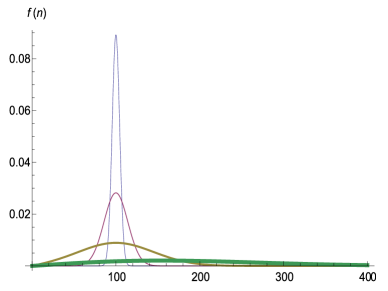
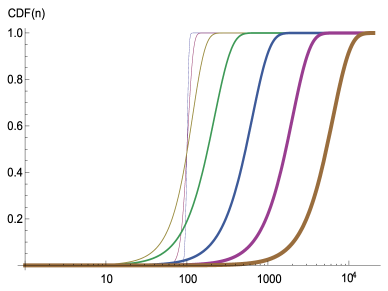
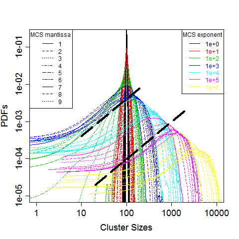
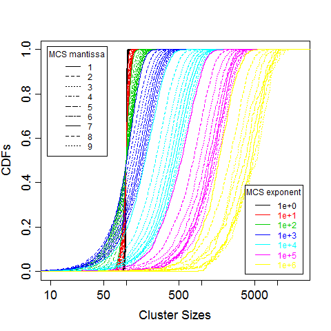
From practical point of view it is not easy to distinguish scaling laws (8) and (9) and difference between them by analysis of probability density functions (PDFs) for various moments of time (Fig. 2a), especially from scarce and noisy experimental data. But it is much more easier to observe the scaling laws by analysis of the cumulative distribution functions. For example, the visual comprehension of scaling law (9) can be easily obtained by viewing the steady shift of the correspondent cumulative distribution functions (CDFs) to the right side in Fig. 2b. The shift becomes diffusive (i.e. proportional to ) after , when the first cluster will reach the 0-boundary, i.e. by continuous detachments some cluster will decrease its size to 0 and disappear.
It means that one can determine the qualitatively different scaling regimes — “infinite” (8) and “semi-infinite” (9) — in this aggregation model with additive rules by the scaling analysis of the probability distribution function for high values of . As it will be shown below in section 4.1, scaling analysis of cumulative density functions is more efficient for practical purposes. The unbounded case (Cauchy problem for infinite domain corresponds to a situation with the constant number of clusters (monomers only redistribute between them), and the bounded one (first boundary value problem for domain — to a situation with irreversible decrease of the number of clusters.
Wall - maximum active surface
For the case clusters have the maximum active surface and under condition one can get:
| (10) |
which has numerous particular solutions that are dependent on the initial and boundary conditions. Again for illustrative purpose we consider the time evolution of the initial singular distribution of clusters of the same size ( that exchange the monomers. It is actually the first boundary value problem for domain , , with the following solution:
| (11) |
Again, on the initial stage of this one-step aggregation process the probability distribution function does not “feel” the boundary condition , because from the physical point of view the cluster size cannot reach the boundary immediately, but only after some time , when the first cluster disappear due to detaching monomers. When all clusters have nearly the same size , and the solution of (10) has not influenced by differences in significantly and that is why it has approximate solution, which is close to solution of the heat equation (7):
| (12) |
| (13) |
Thus, again in the same process we have change of size distribution (from (12) to (13)) and scaling law (from (14) to (15)) driven by 0-boundary condition for the probability distribution function of walls for :
-
1.
from “infinite” diffusive scaling law for
(14) -
2.
to “semi-infinite” ballistic (linear) scaling law for and
(15)
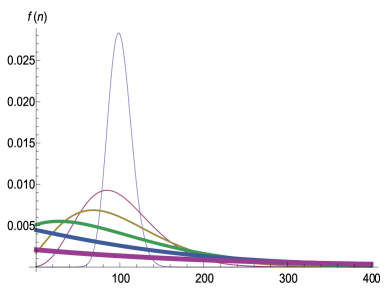
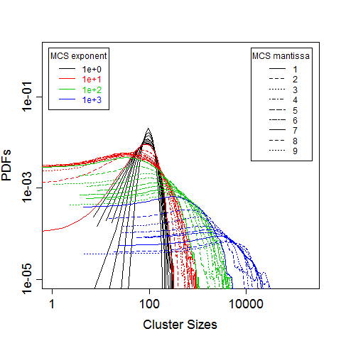
Again, as in the case with pile-ups, it is not easy to distinguish scaling laws (14) and (15) and difference between them by analysis of PDFs for various times (Fig. 3a), especially from experimental data.
a) b)
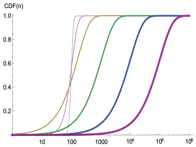
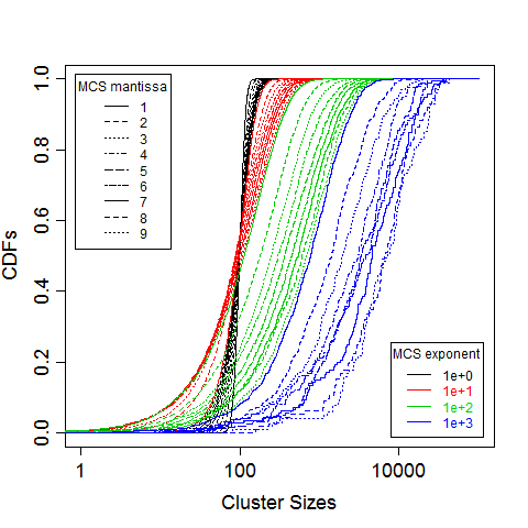
And it is much more easier to observe the scaling laws by analysis of the cumulative distribution functions (Fig. 3b). The visual comprehension of scaling law (15) can be easily obtained by viewing the steady shift of the cumulative distribution functions (CDFs) to the right side in Fig. 3b. The shift becomes linear (i.e. proportional to ) after (but not after , like it was for pile-ups!), when the first cluster will reach the 0-boundary, i.e. when some cluster by continuous detachments will decrease its size to 0 and disappear. But the most essential point is that shortly after the size distribution for wall configuration becomes exponential (13), that is scale-free one and without any “apparent” peak value.
The assumption as to the better scaling analysis of CFDs in comparison to PDFs is related to the following simple property: if PDF is scaled by some law like , than its CDF is scaled by the following law:
| (16) |
This means that if PDF can be scaled by stretching its ordinates () and abscissas (), then its CDFs can be scaled by stretching abscissas () only, but not by ordinates (), which will be preserved.
Thus, change of scaling for pile-up CDF should be:
-
1.
from “infinite” diffusive scaling law for
(17) -
2.
to “semi-infinite” diffusive scaling law for
(18)
Similarly, change of scaling for wall CDF should be:
-
1.
for (“infinite” diffusive scaling law)
(19) -
2.
for and (“semi-infinite” ballistic (linear) scaling law)
(20)
In comparison, nonlinear Leyvraz–Redner approach [5] on the basis of the linked Smolukhovski nonlinear equations [22] becomes linear (under conditions of the product kernel and conserved number of all monomers ) after rescaling the time variable by moments of the size distribution , as it was shown in similar Ben-Naim-Krapivsky theory for exchange driven growth [18] and Lin-Ke theory for migration-driven aggregation [19, 20, 21], which were also formulated on the basis of the linked Smolukhovski nonlinear equations [22]. The one-step model proposed here is in agreement with results of scaling analysis on the basis of the approximate ansatz function in Ben-Naim-Krapivsky theory for exchange driven growth, namely with Eq.(8) and Eq.(10) in their work [18] taking into account the rescaled time variable. Moreover, the rescaled time variable in Eq.(3) in Ref.[18] expresses the essential difference between the one-step formulation of aggregation process proposed here (where single transitions allowed and between adjacent integers only [23], which manifests itself in linearity and ) and the multi-step formulation of aggregation process [5, 19, 20, 21] (where multiple transitions allowed and between any integers, which manifests itself in non-linearity, , and time dependence on the available cumulative active surface expressed by multiplier in Eq.(3) in Ref.[18]).
One of drawbacks of the simplified model is that the equations (4) and (10) and their solutions (5) and (11) give the idealized and rough representation of the aggregation kinetics. In fact, solutions (5) and (11) allows the “long-tails” of distribution, i.e. non-zero density of clusters for arbitrary high or low values of in the ranges and for any stage of evolution. For example, any initial cluster of size will need at least detachment steps to disappear. But the analytical solution (5) gives the non-zero values of cluster distribution for any small , i.e. does not prohibit immediate disappearance of this initial cluster even at the first step after start of the aggregation process. In a real physical process it is impossible due to physical limitations of diffusive character of the one-step aggregation process among clusters with pile-up morphology. This situation is well-known and actively investigated in the class of so-called ”first-passage problems” [23]. That is why, the analytical solutions and predictions of the model cannot be directly applied to the correspondent practical situations without taking into account the limits of their physical counterparts. Below, the aforementioned change of size distribution and scaling law driven by 0-boundary condition is investigated by the following simulations.
3 Simulation
The two aforementioned primitive cases of cluster aggregation were simulated by Monte Carlo method to illustrate the different cluster distributions in different aggregation kinetics. The numerous initial configurations of clusters with various numbers of monomers in each of them were used in simulations with a conserved number of aggregating monomers as a whole. Below the results on initial configurations of clusters with monomers are considered (and the other vast configurations will be reported later [26]). Further the analytical calculations in section 2 will be compared with the results of simulation and for this purpose the number of Monte Carlo sweeps (MCSs) will be assumed to equal to the number of time steps . All simulation runs were performed in the distributed computing infrastructure (DCI) “SLinCA@Home” (Scaling Law in Cluster Aggregation) (http://dg.imp.kiev.ua/slinca) on the basis of BOINC SZTAKI Desktop Grid (DG) technology [31, 32] through the linked science gateway portal on the basis of WS-PGRADE technology [33].
Pile-up — minimum active surface
a) b)
The “pile-up” aggregation of monomers (see Fig. 1a) has a minimum active surface and it was simulated for unbiased migration-driven aggregation. The kinetics of rearrangements from the initial configuration is shown in Fig.4. After some MCSs of the initial configuration the broad peak appears, which corresponds to the average cluster size. The size distributions of pile-ups (Fig. 4a) become asymmetric, but they preserve their one-peak shapes. And their CDFs (Fig. 4b) demonstrate the “diffusive” scaling law, which becomes evident after some number of MCSs, namely after . It can be seen visually by the shift of the simulated CDFs to the right side (proportionally to ) on the log-linear plot in (Fig. 4b) and can be compared with the same shift of the analytically calculated CDFs in Fig. 3b. The two straight thick dash lines are given in Fig. 4a as a guide for eyes to emphasize that for and , that is follows from (6).
Wall — maximum active surface
a) b)
The “wall” aggregation of monomers (see Fig. 1b) has a maximum active surface and it was simulated for unbiased migration-driven aggregation. The kinetics of rearrangements from initial configurations is shown in Fig. 5. It can be seen that size distributions of walls (Fig. 5a,b) become asymmetric also. Moreover, they do not preserve their one-peak shapes after some number of MCSs and become scale-free, as it was predicted by the analytical solution (13) for . After some Monte Carlo sweeps (MCSs) the initial peak, that corresponds to the initial cluster size , disappear and the scale-free distribution without distinctive peak appears. This transition is much more evident in the log-log representation of cluster size distributions on Fig. 5a, where availability of peak (after ) is apparent, such “peak” cannot be distinguished from error limits, and its position is highly dependent on the selected bin size. Their CDFs (Fig. 5b) also demonstrate the “semi-infinite” ballistic (linear) scaling law (15), which becomes evident after some number of MCSs, when the shift of CDFs to the right side of the plot in Fig. 5b becomes linearly proportional to after . One can easily compare it with the similar shift of CDFs in Fig. 3b).
To avoid the subjective estimations (like visual examination) of PDF/CDF curves, the simulation results were analyzed by the scaling, fitting, moment, and bootstrapping analysis in the next sections.
4 Change of scaling and distribution type
4.1 Scaling analysis
Comparison of analytical and simulation results shows that monomer aggregation (at least, in pile-up and wall configurations of clusters) can be satisfactorily described by the proposed theoretical model of one-step aggregation processes. The important thing is that some scaling laws can be determined experimentally by scaling analysis of size distributions (PDFs and CDFs) of the real aggregating ensembles. Below some attempts of such analysis for 63 different pile-up PDF/CDF pairs and for 36 different wall PDF/CDF pairs are shown on the basis of aforementioned simulation results and with usage of R language and environment for statistical computing [34].
Pile-up — minimum active surface
a) b)
c) d)
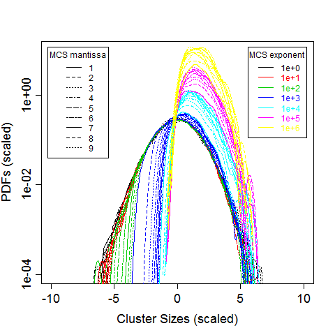
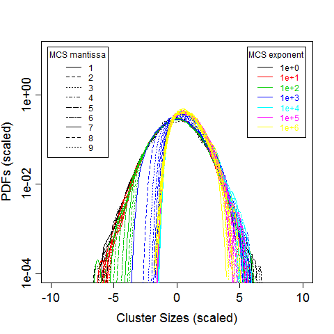
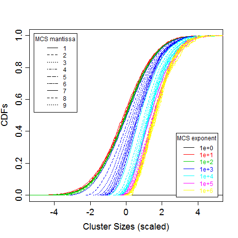
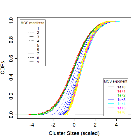
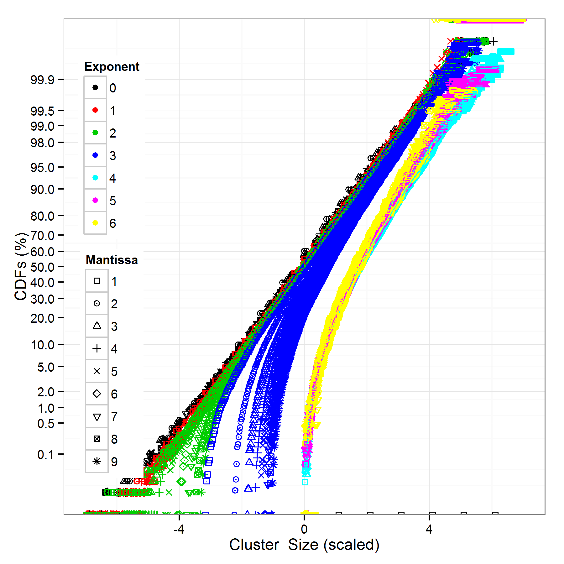
Application of two scaling laws (“infinite” (8) for and “semi-infinite” (9) for ) to simulated PDFs (Fig. 6a), and scaling laws (“infinite” (17) for and “semi-infinite” (18) for ) — to simulated CDFs (Fig. 6c) of pile-ups shows the clear difference between these two scaling regimes. The “infinite” diffusive scaling law (8) corresponds to the initial stage (in the range of MCS steps ), i.e. the 18 scaled PDFs (Fig. 6a) and CDFs (Fig. 6c) curves collapse to the initial symmetric size distribution. Some inclinations from perfect collapse are related to influence of the boundary condition and slow transition to the different scaling law (for the left tail), and worse precision, because of the low number of biggest cluster (for the right tail). The same collapse of the scaled CDF curves to the initial straight line can be seen on the probability plot (Fig. 7a). The straight dashed line on the probability plot corresponds to CDF of normal distribution, i.e. this collapse demonstrates good correspondence to solution (7).
a) b)
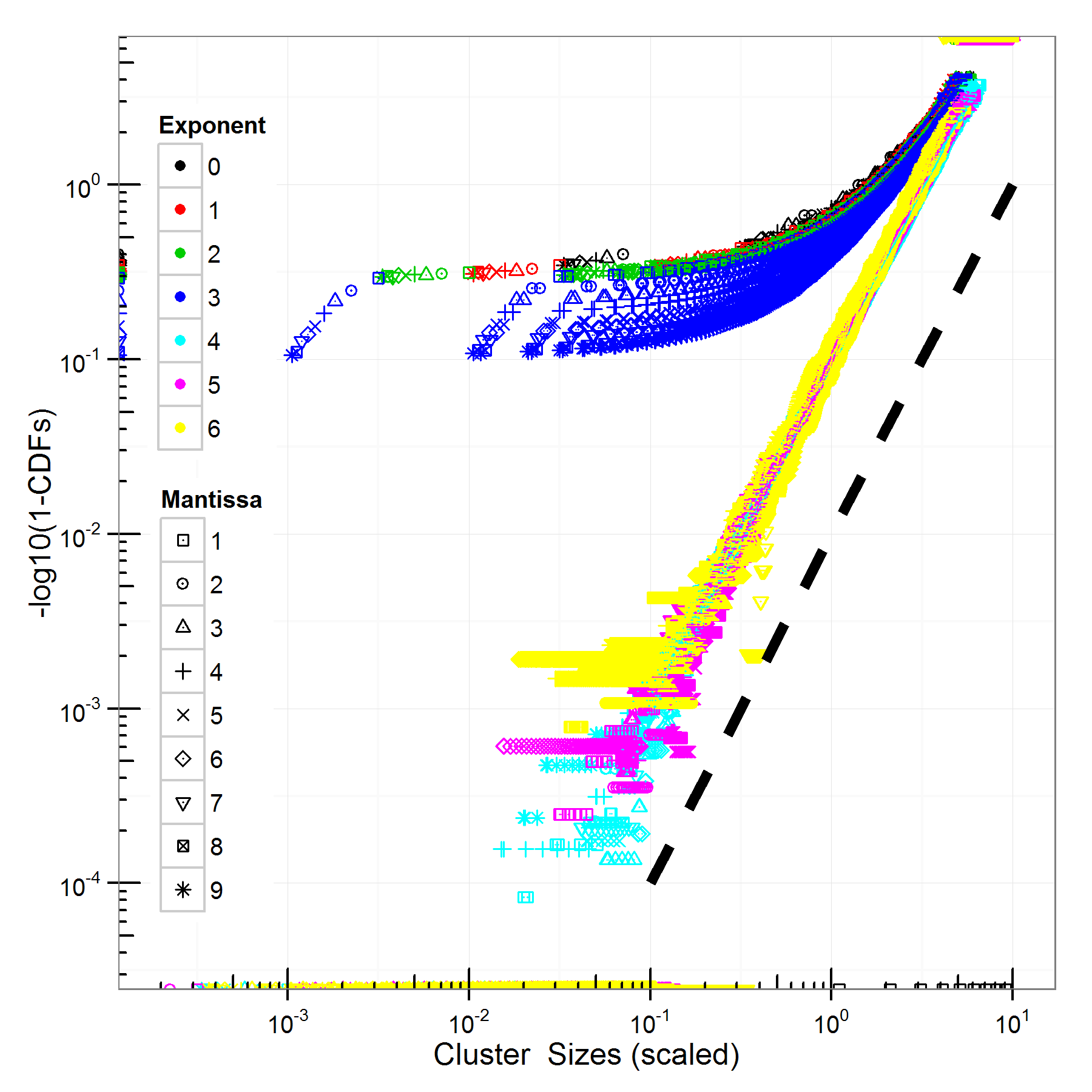
The “semi-infinite” diffusive scaling law (9) takes place later (in the range of MCS steps ), i.e. the scaled PDFs (Fig. 6a) and CDFs (Fig. 6c) curves collapse to the asymptotic asymmetric size distribution. The same collapse of the scaled CDF curves to the asymptotic straight line can be seen on the plot (Fig. 7b) with the scaled ordinate axis (see the label near this axis). The straight dashed line on such plot corresponds to CDF of Weibull distribution, which slope ( in Fig. 7b) should correspond to the power of under exponent in (6) (see the details in [26], namely, Eq.(5) and Eq.(6)). This collapse demonstrates good correspondence to solution (6), and the detailed comparison of Weibull distribution and solution (6) will be given below in section 4.2.
The approximate transition region () between these two scaling laws can be observed in Fig. 6a,c and Fig. 7 as the 15-20 shifting to right curves (denoted by blue color in electronic version), i.e. near the moment of the first-passage of a cluster through the point of disappearance (). The matter is after reaching the 0-boundary () the number of clusters decreases and the mean of the cluster distribution increases like . Thus, the PDFs and CDFs (mostly corresponding to solution (5) with taking into account ) can be scaled to the better collapse near peaks (Fig. 6b,d) by the other “diffusive scaling law with moving mean”:
| (21) |
It should be emphasized that this “diffusive scaling law with moving mean” is good for the regions near peak of distribution () and bad for the right tail () (see Fig. 6b).
Wall — maximum active surface
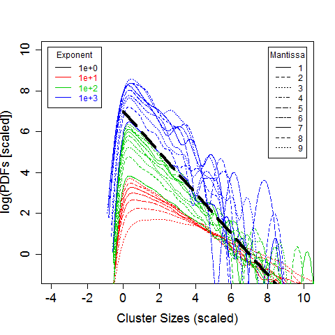
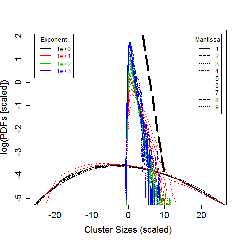
Similarly, application of of two scaling laws (“infinite” diffusive (14) for and “semi-infinite” ballistic (linear) (15) for to simulated PDFs (Fig. 8) and CDFs (Fig. 9) of walls shows the other clear difference between two scaling regimes. The “infinite” diffusive scaling law (14) corresponds to the initial stage , i.e. the 9 scaled PDFs collapse to the initial symmetric size distribution in Fig. 8b; and the 9 scaled CDFs — to the initial straight line on the probability plot in Fig. 9a. The “semi-infinite” ballistic (linear) scaling law (15) takes place later (for after some transient period. The 18 scaled PDFs are attracted to the other asymmetric and scale-free size distribution, which is actually the exponential one (see tendency for the right tails in Fig. 8); and the 18 scaled CDFs — to the asymptotic straight line on the plot (Fig. 9b) with the Weibull-scaled ordinate axis (see the label near this axis). The straight dashed lines in Fig. 8 corresponds to PDF of exponential distribution, which slope ( in Fig. 8) should correspond to the power of under exponent in (13).
a) b)
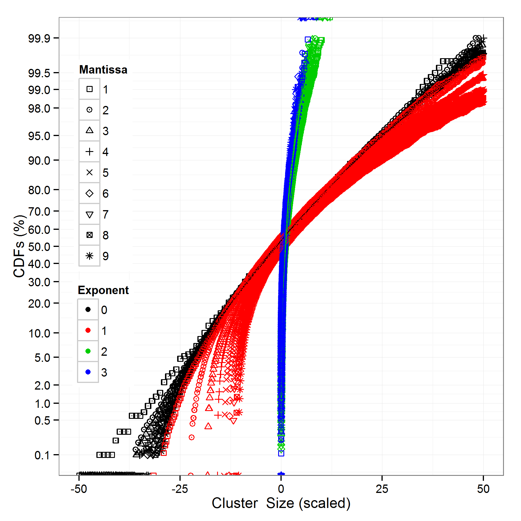
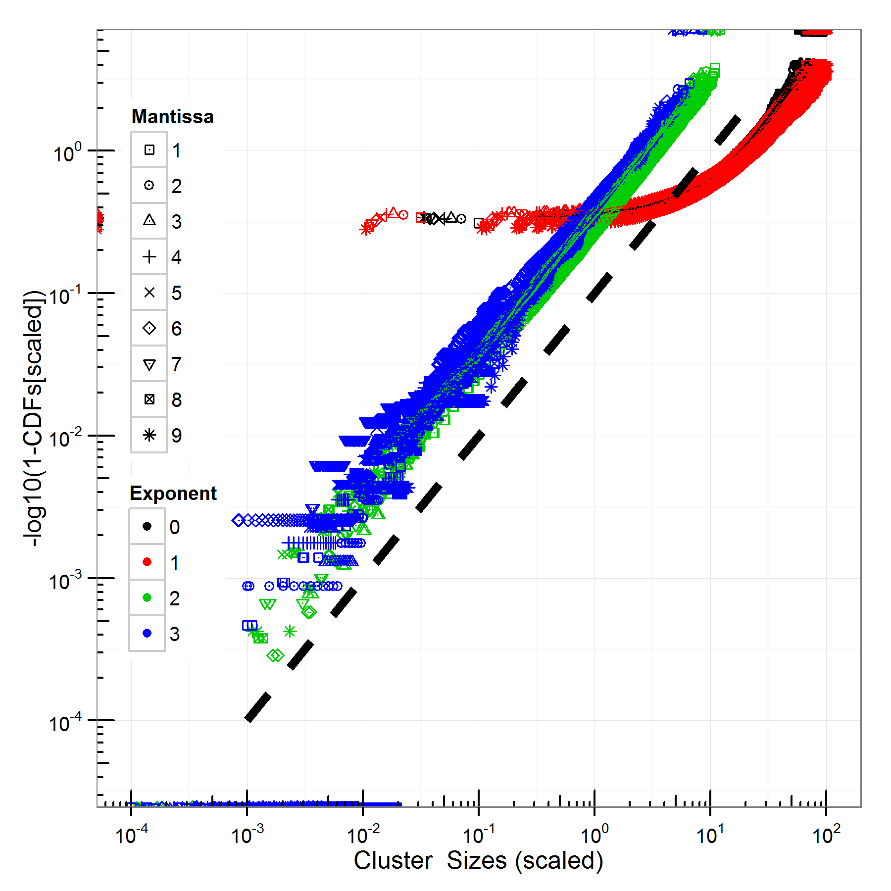
a) b)
It should be noted that scaling laws (14) and (15) are not universal for all and , because they were derived from the approximate solutions (12) and (13). Moreover, the exact solution (11) of equation (10) contains several combinations of and (like , , ), that will not allow for simple scaling transformation for all and . As a result some limiting cases can be emphasized, for example, collapse of scaled curves in Fig. 8a is not good enough, because for the Bessel function for and asymptotic version of solution (2) will be close to:
| (22) |
And PDFs should be better scaled by the other scaling law:
| (23) |
The PDF curves scaled by this law (Fig. 8b) demonstrates a good collapse and correspondence to the asymptotic solution (18). It should be noted that PDF is sensitive to the shape (type) of the distribution and CDF is not, which allows us to find the change of scaling by analysis of CDFs with a higher precision and reliability, than by analysis of PDFs.
Really, the collapse of the scaled CDF curves to the initial straight line can be seen on the probability plot (Fig. 9a). The straight dashed line on the probability plot corresponds to CDF of normal distribution, i.e. this not-perfect collapse demonstrates very rough correspondence to the approximate solution (12) and for the initial stage only (). This unsatisfactory scaling is explained by the appearing difference in the cluster sizes, when the initial approximation becomes not accurate. That is why (10) becomes influenced by differences in significantly and that is why its approximate solution (12), which is close to solution of the heat equation (7) becomes more inaccurate with time, especially for tails, where difference in is bigger. The same collapse of the scaled CDF curves to the asymptotic straight line can be seen on the plot (Fig. 9b) with the Weibull-scaled ordinate axis (see the label near this axis). The straight dashed line on such plot corresponds to CDF of Weibull (actually exponential one) distribution, which slope ( in Fig. 9b) should correspond to the power of under exponent in (13). This collapse of 20 scaled CDF curves (in the range of 2 decades of MCSs) demonstrates a good correspondence to solution (13), and the detailed comparison of Weibull distribution and solution (13) will be given below in section 4.2.
On practice, when the actual analytic solutions, scaling laws, and availability of such boundary are not known, such scaling analysis (even for CDFs) can be a very hard and unproductive task. It is exacerbated by the everlasting problem, because visual examination of data collapse on the same scaling curve has the subjective nature. Below, some other useful tools are proposed to determine the boundary-driven change of scaling and type of distribution.
4.2 Analysis of fitting distributions
According to scaling analysis of asymptotic behavior of pile-ups and walls, their PDF/CDF pairs should change crucially after transition period and , respectively.
Pile-up — minimum active surface
| (24) |
where is a Weibull distribution (where is a shape parameter and is a scale one), and its CDF will be:
| (25) |
which is the exact CDF for a Weibull distribution with .
Wall — maximum active surface
Similarly, after substitution the PDF from (13) will be:
| (26) |
where is a Weibull distribution, actually the exponential distribution for (where is a shape parameter and is a scale one), and its CDF will be:
| (27) |
which is the exact CDF for a Weibull distribution with .
This means that the change of scaling could be determined by the change: from the initial normal distribution for pile-ups (or close to normal for walls) to Weibull distributions with the different constant shape parameters and the scale parameters for pile-ups ( for walls), which should differently change with time after transition period for pile-ups (and for walls).
a) b)
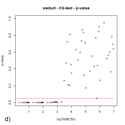
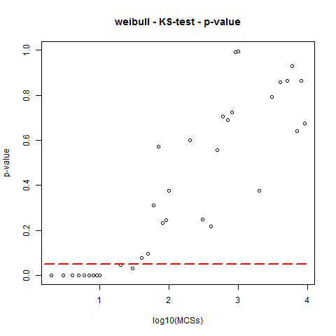
Despite the visually good collapse of CDF curves in Fig.7b and Fig.9b, where the ordinate axes are fitted so, that the straight dashed lines correspond to Weibull distributions, the goodness of fits (25) and (27) was checked in the following statistical test. The null and alternative hypotheses were:
-
1.
: Data come from the Weibull distributions,
-
2.
: Data do not come from the Weibull distributions.
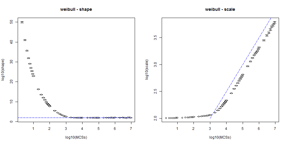
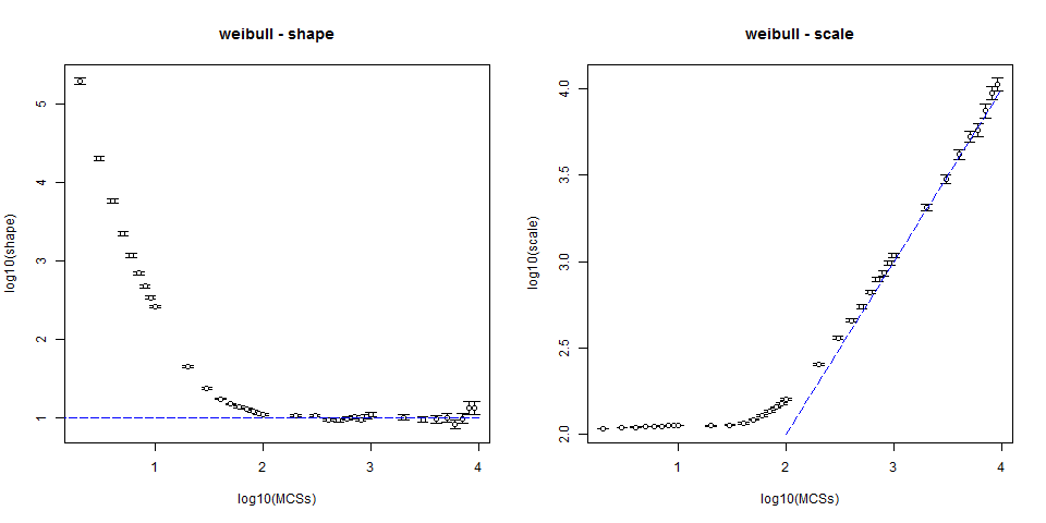
The Kolmogorov-Smirnov (KS) test [35, 36, 37] was used to decide if simulated data comes from a population with Weibull distributions, which is based on a comparison between the simulated CDFs in Fig.4b and Fig.5b and theoretical Weibull CDFs from (25) and (27). From Fig.10 one can see that p-values are higher than significance level of 0.05 (noted by dash line) usually referred in statistical literature. The higher values of p-value in the KS-tests mean the higher probabilities of wrong rejection of the fitting -hypothesis. But the p-values higher that the typical significance level () do not obligatory mean that the hypothesis is absolutely true. Rather, the higher p-value for the hypothesis of the Weibull distribution means the higher probability of wrong rejection of -hypothesis that the estimated distribution follows the Weibull distribution. It means that -hypothesis for the Weibull distribution, i.e. for pile-ups the simulated data (Fig.4b) come from the Weibull distribution, can be accepted in the range of MCSs, where , and for walls the simulated data (Fig.5b) come from the Weibull distribution, can be accepted in the range of MCSs, where . Namely, CDFs of pile-ups (Fig.4b) could be Weibull ones for , that agrees with the stated Weibull-like asymptotic (25) for . And, CDFs of walls (Fig.5b) could be Weibull ones for , that agrees with the stated Weibull-like asymptotic (27) for .
According to (24) fitting pile-up PDFs to Weibull distribution for should give the constant shape parameter, i.e. equal to , and the following dependency for scale parameter . This assumption is supported by the pile-up simulated data (Fig.11) for , where (the horizontal dashed line in Fig.11a denotes 2 on the ordinate axis) and (the slope of the dashed line in Fig.11b is 1/2).
a) b)
a) b)
According to (26) fitting wall PDFs to Weibull distribution for should give the constant shape parameter, i.e. equal to 1, and the following dependency for scale parameter . This assumption is supported by the wall simulated data (Fig.12) for , where (the horizontal dashed line in Fig.12a denotes 1 on the ordinate axis) and (the slope of the dashed line in Fig.12b is 1).
In general sense, this means that fitting analysis (with KS-test and analysis of evolving distribution parameters like shape-scale for the Weibull distributions) can be used as an additional useful tool for investigation of any changes of distribution type and related scaling law (like the boundary-driven change presented here).
4.3 Moment analysis
The moments like mean , variance (square of standard deviation ), excess , and kurtosis are of great interest, because they are measurable in experiments, are not so vulnerable to fluctuations in empirically constructed PDFs, follow the general scaling law, and have the clear physical sense.
Pile-up — minimum active surface
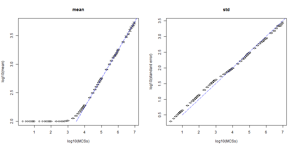
For pile-ups, from (7) for the mean cluster size is constant and its standard deviation grows like , and it is true for the pile-up simulated data (Fig.13), where and for . But after transition region it follows from (24) that the mean cluster size is and its standard deviation grows like , and it is true for the pile-up simulated data (Fig.13), where and for .
a) b)
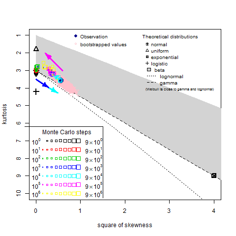
The higher standardized moments of pile-up size distributions, namely skewness and kurtosis , have the following forms for (24) for :
| (28) |
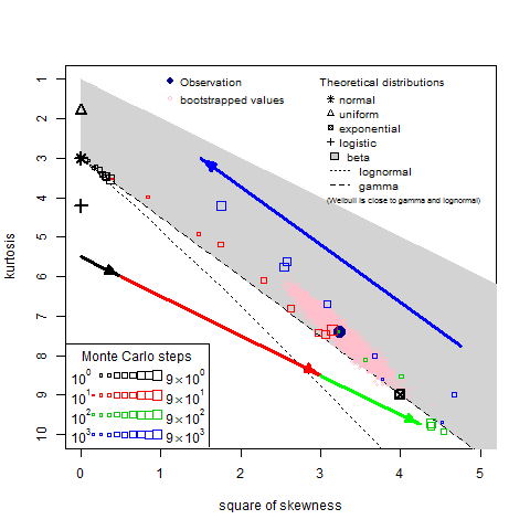
After simple calculations the square of skewness is equal to , and kurtosis is equal to . On the Pearson diagram (Fig. 14) [38, 40, 39] each data point (square) represents moments (kurtosis and square of skewness ) of the certain simulated PDF for some stage of the aggregation process. The color of square (in electronic version) denotes exponent, and the relative size of square (see legend) — mantissa of MCSs in decimal logarithmic notation. For example, the smallest red square corresponds to PDF for and the biggest red square — to PDF for . The data on the Pearson diagram clearly demonstrate the change of the distribution type: for more than 30 pile-up PDFs collapse to the initial normal distribution (near point with coordinates: kurtosis and square of skewness ) and after pile-up PDFs migrate to the zone of Weibull distributions (near point with coordinates: kurtosis and square of skewness ).
Wall — maximum active surface
For walls, from (14) for the mean cluster size is constant and its standard deviation grows like , and it is true for the wall simulated data (Fig.15) for . But after transition region from (26) follows that the mean cluster size and its standard deviation should grow like , and it is true for the wall simulated data (Fig.15) where and for .
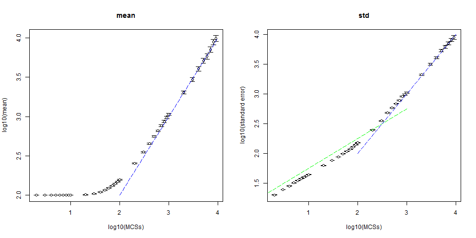
a) b)
The higher standardized moments of wall size distributions, namely skewness and kurtosis , have the similar forms as in (4.3). And after simple calculations the square of skewness is equal to , and kurtosis is equal to . They are presented on the Pearson diagram (Fig. 16) and demonstrate the change of the distribution type: for distributions are collapsed to the initial normal distribution (near point with coordinates: kurtosis and square of skewness ) and after they quickly migrate through the zone of Weibull distributions to the location of exponential distribution denoted by black square with circle and cross inside (near point with coordinates: kurtosis and square of skewness ).
The other interesting aspect is the reverse migration of distributions denoted by the backward arrows on the Pearson diagrams: the magenta arrow for pile-ups in Fig.14 and the blue arrow for walls in Fig.16. They correspond to the very late behavior of the simulated systems with the limited quantity of particles , when the most part of time the ensemble of large clusters exchange by particles without total disappearance of any cluster. This means clusters do not “feel” the 0-boundary and the third problem with “infinite” boundary conditions should be considered for equations (4) and (10). As a result these PDFs become more symmetric (lower skewness) and with quasi-normal peaks (lower kurtosis). But the whole consideration of this third problem is beyond the scope of this article and will be considered elsewhere.
In total, the moment analysis allow to identify the 0-boundary driven changes of distribution type and related scaling law by the crucial changes of moments, like mean , variance (square of standard deviation ), excess , and kurtosis after transition times and .
4.4 Bootstrapping analysis
To check the stability of the simulated distributions shown on the Pearson diagram the bootstrapping analysis [39] was applied in order to simulate the exclusion of some clusters from the cluster distribution. The results of the bootstrapping analysis for some PDF is plotted on the Pearson diagram (Fig. 14 and Fig. 16) as a pink area of scattered dots. Each pink dot corresponds to pair of skewness and kurtosis values, which is calculated for each of many bootstrap samples.
For example, for the pile-up PDF on the Pearson diagram in Fig. 14 the results of the bootstrapping analysis for are plotted as a pink ellipse of scattered dots. Each pink dot corresponds to pair of skewness and kurtosis values, which is calculated for each of bootstrap samples. It is important to note that the bootstrapping area for the initial stage has the equiaxial circular shape (it is not shown here) and it is located near the point of the normal distribution: kurtosis and square of skewness . While the bootstrapping area for is stretched and located in the zone of Weibull distributions near the point with coordinates: kurtosis and square of skewness .
Similarly, for the wall PDF on the Pearson diagram in Fig. 16 the results of the bootstrapping analysis for are plotted as a more elongated pink ellipse of scattered dots. It is important to note that the bootstrapping area for the initial stage has the equiaxial circular shape (it is not shown here) and it is located near the point of the normal distribution: kurtosis and square of skewness . And the bootstrapping area for is stretched to the location of exponential distribution (black square with circle and cross inside) near point with coordinates: kurtosis and square of skewness .
Finally, this means that bootstrapping analysis allow to estimate the stability of the estimated moments for the simulated distributions, determine the areas of their possible locations on the Pearson diagram, and identify the 0-boundary driven changes of distribution type and related scaling law by crucial change of the positions and shape of the bootstrapped sample areas in coordinates on the Pearson diagram.
5 Discussion
| Example | Parameter | Value for | No. | |
| Scaling analysis (section 4.1) | ||||
| Pile-ups | (1) | |||
| — | 18 | 30 | (2) | |
| — | (3) | |||
| — | 18 | 30 | (4) | |
| Walls | (5) | |||
| — | 9 | 18 | (6) | |
| — | (7) | |||
| — | 9 | 18 | (8) | |
| Fitting analysis (section 4.2) | ||||
| Pile-ups | (9) | |||
| Walls | (10) | |||
| Moment analysis (section 4.3) | ||||
| Pile-ups | (11) | |||
| — | (12) | |||
| — | 0 | 0.632 | (13) | |
| — | 3 | 3.25 | (14) | |
| Walls | (15) | |||
| — | (16) | |||
| — | 0 | 2 | (17) | |
| — | 3 | 9 | (18) | |
| Bootstrapping analysis (section 4.4) | ||||
| Pile-ups | normal | Weibull | (19) | |
| Walls | normal | exp Weibull | (20) | |
Scaling analysis of simulated (or experimentally obtained) size distributions and histograms (PDFs) is very hard and prone to errors task, because of the some uncertainty related to proper and optimal binning procedures for preparation of histograms. In contrast, the scaling analysis of experimental and simulated CDFs has much higher stability to statistical deviations and outliers among data. It is partially explained by the absence of shape scaling (2). The better collapse of scaled CDF curves could be seen even by visual comparison of scaled simulated histograms (PDFs) (Fig. 6a,b and Fig. 8) with their scaled CDFs (Fig. 6c,d, Fig. 7, and Fig. 9).
The initial “singular” configurations of walls after some time sweeps evolve to scale-free distributions (Fig. 8), that is different from pile-up distributions with broad peaks for the same time (Fig. 6a). That is why in practical sense the notion of “average cluster size” seems to be meaningless for this kind of cluster size distributions (i.e. for exponential-like wall arrangements) without distinctive peaks. This observations can give some insights as to possible roots for self-affine arrangements of defects and their manifestations at the surface of plastically deformed metals.
In general, the boundary driven change of scaling and distribution type at can be identified by more than 10 parameters summarized in Table 1 for 2 examples of aggregation kinetics for clusters with pile-up and wall morphology. That is why in practice to estimate scale invariant characteristics of systems and their changes (e.g. the level of hierarchy of defect substructures and related scale of damage) it is necessary to measure and analyze not only the integral “averaged” characteristics of defect ensembles (density per area, average size, etc.), but also to define more specific characteristics, related with their size distributions, like PFDs/CDFs and their parameters [41]. Moreover, scaling, fitting, moment, and bootstrapping analysis can be very informative and useful for the more detailed and precise analysis of evolving distributions. One of the examples of such scaling analysis applied for CDFs was demonstrated for statistical analysis of features observed on surfaces of plastically deformed Al single crystals under real-time video monitoring and processing [42], Another example of such scaling and statistical analysis (Kolmogorov-Smirnov test of fitting, moment analysis, and bootstrapping analysis) was proposed for the defect density distribution over the ensemble of nanocrystals. And it had shown that change of plastic deformation mode is followed by the qualitative change of defect density distribution type over ensemble of nanocrystals [43].
It should be noted that the mean cluster size grows in agreement with conclusions of nonlinear Leyvraz-Redner scaling theory [5] about average aggregate growth like . Also conclusions for the partial cases (pile-ups and walls) considered here are in agreement with conclusions on an average cluster size in Lin-Ke theory for migration-driven aggregation, namely pile-ups () grow as (diffusive growth [19]) and walls () grow as (ballistic growth [20]). Also the results stated here are in agreement with scaling estimations of the typical scale growth for diffusive and ballistic regimes in Ben-Naim-Krapivsky theory for exchange driven growth [18] taking into account the rescaled time variable.
In the more general sense, scaling, fitting, moment, and bootstrapping analysis of experimental distributions could allow us to determine their intrinsic symmetry and bring to light the corresponding aggregation scenario for many other applications related with aggregation phenomena, for example for investigation of city population dynamics [27].
At the moment some outliers and unsatisfactory scaling in the simulation data cannot be compared directly with the theoretical results for large and because simulations were carried out for relatively low number of aggregating monomers (10 and in the limited time range ( MCSs for pile-ups and MCSs for walls). That is why to check the exact solutions and make more reliable conclusions the bigger simulations are under way now in the DG DCI “SLinCA@Home” and the science gateway portal on the basis of WS-PGRADE technology[44].
6 Conclusions
The idealized general model of one-step processes to characterize aggregate growth was proposed that allowed us to find the scaling characteristics of some aggregation scenarios. Some factors that can cause scaling transition and appearance of the self-affine size distribution of the aggregating system of solitary agents (monomers) and their aggregates (clusters) were brought to light: the rate of monomer exchange between clusters, cluster geometry, and initial cluster size. It was shown that the simplified aggregate growth can be described by the one-variable Fokker-Planck equation in general form with time-independent drift and diffusion coefficients. In some aggregation scenarios it could be transformed to the equivalent equations, from which the non-stationary analytical solutions with some initial and boundary conditions can be obtained.
Two primitive cases of cluster aggregation were considered analytically and simulated by Monte Carlo method to illustrate the different cluster distributions in different aggregation kinetics: model with minimum active surface (singularity) that corresponds to “pile-up” aggregation of dislocations, and model with maximum active surface that corresponds to “wall” aggregation of dislocations. It was shown that initial “singular” symmetric distribution of pile-ups evolves according to “infinite” diffusive scaling law and later it is replaced by the other “semi-infinite” diffusive scaling law with asymmetric distribution of pile-ups. In contrast, the initial “singular” symmetric distributions of walls initially evolve according to the diffusive scaling law and later it is replaced by the other linear scaling law with scale-free exponential distributions without distinctive peaks.
The scaling, fitting, moment, and bootstrapping analysis were proposed for the simulated data to identify the 0-boundary driven change of scaling and distribution type at by the abrupt change of parameters: PDF scaling law (No.1,5 in Table 1), PDF shape (1,5), number and time range of collapsed PDFs (2,6), CDF scaling law (3,7), CDF shape (3,7), number and time range of collapsed PDFs (4,8), p-value in KS-test of fitting CDFs (9,10), mean (11,15), standard deviation, which does not change for pile-ups (12,16), skewness (13,17), kurtosis (14,18), locations of the bootstrapped samples in coordinates on the Pearson diagram (19,20).
From the practical point of view and in the more general sense, scaling, fitting, moment, and bootstrapping analyses of experimental distributions of aggregating monomers and clusters will allow to determine their intrinsic symmetry, bring to light the corresponding aggregation scenario, and influence of aforementioned parameters (rate of monomer exchange between clusters, cluster geometry, and initial cluster size).
7 Acknowledgements
The work presented here was partially funded by the EU FP7 DEGISCO (Desktop Grids for International Scientific Collaboration) (http://degisco.eu) project, which is supported by the FP7 Capacities Programme under grant agreement number RI-261561; EU FP7 SCI-BUS (SCIentific gateway Based User Support) project, contract no. RI-283481; and partially supported in the framework of the research theme “Introduction and Use of Grid Technology in Scientific Research of IMP NASU” under the State Targeted Scientific and Technical Program to Implement Grid Technology in 2009-2013. The special thanks should be expressed to the community of volunteer supporter of the the DG DCI “SLinCA@Home”, and especially “Distributed Computing team “Ukraine”” (http://distributed.org.ua) for their computing resources generously donated for calculation of some of these results.
References
- [1] I. Lifshitz and V. Slyozov, Zh. Eksp. Teor. Fiz. 35, 479 (1958) (in Russian); The kinetics of precipitation from supersaturated solid solutions, J. Phys. Chem. Solids 19 (1961) 35–50.
- [2] A. Zangwill, Physics at Surfaces, Cambridge University Press, New York, 1988.
- [3] S. Chandrasekhar, Stochastic problems in physics and astronomy, Rev. Mod. Phys. 15 (1) (1943) 1–89.
- [4] S. Ispolatov, P. Krapivsky, S. Redner, Wealth distributions in asset exchange models, Eur. Phys. J. B 2 (1998) 267–276.
- [5] F. Leyvraz, S. Redner, Scaling theory for migration-driven aggregate growth, Phys. Rev. Lett. 88 (6) (2002) 68301.
- [6] B. Mandelbrot, D.E. Passoja, A.J. Paullay, Fractal character of fracture surfaces of metals, Nature 308 (1984) 721–722.
- [7] S. Stach, J. Cybo, Multifractal description of fracture morphology: theoretical basis, Mater. Charact. 51 (2003) 79–86.
- [8] S. Stach, S. Roskosz, J. Cybo, J. Cwajna, Multifractal description of fracture morphology: investigation of the fractures of sintered carbides, Mater. Charact. 51 (2003) 87–93.
- [9] Y. Gordienko, E. Zasimchuk, Single-crystal indicators of fatigue and plastic deformation damage, Proc. SPIE 2361, Second European Conference on Smart Structures and Materials, (1994) 312–315.
- [10] Y. Gordienko, E. Zasimchuk, T. Turchak, Scaling of structural parameters and mechanical properties of metals and alloys, Physical Mesomechanics 10 (3-4) (2007) 129–133.
- [11] Y. Gordienko, P. Kuznetsov, E. Zasimchuk, R. Gontareva, J. Schreiber, V. Karbovsky, Multiscale 2D Rectangular and 3D Rhombic Gratings Created by Self-Organization of Crystal Structure Defects under Constrained Cyclic Deformation and Fracture, Materials Science Forum 567 (2008) 421–424.
- [12] T. Kleiser, B. Bocek, The fractal nature of slip in crystals, Z. Metallkd. 77 (9) (1986) 582–587.
- [13] H. Neuhäuser, Slip propagation and fine structure, Solid State Phenomena 3 & 4 (1988) 407–415.
- [14] M. Zaiser, F. Grasset, V. Koutsos, E. Aifantis, Self-affine surface morphology of plastically deformed metals, Phys. Rev. Lett. 93 (19) (2004) 195507.
- [15] P. Hähner, K. Bay, M. Zaiser, Fractal dislocation patterning during plastic deformation, Phys. Rev. Lett. 81 (12) (1998) 2470–2473.
- [16] Y. Gordienko, E. Zasimchuk, Synergetic model of structure formation during plastic deformation of crystals, Philosophical Magazine A 70 (1) (1994) 99–107.
- [17] G. Ananthakrishna, Current theoretical approaches to collective behavior of dislocations, Physics Reports, 440 (4) (2007) 113–259.
- [18] E. Ben-Naim, P. Krapivsky, Exchange-driven growth, Physical Review E 68 (3) (2003) 031104.
- [19] J. Ke, Z. Lin, Kinetics of migration-driven aggregation processes, Physical Review E 66 (5) (2002) 050102.
- [20] Z. Lin, J. Ke, Kinetics of a migration-driven aggregation process with birth and death, Physical Review E 67 (3) (2003) 031103.
- [21] Z. Lin, J. Ke, G. Ye, Exchange-Driven Growth with Birth Rate Less Than Death, Communications in Theoretical Physics 43 (5) (2005) 837–840.
- [22] M. Smoluchowski, Drei vortrage uber diffusion, brownsche bewegung und koagulation von kolloidteilchen, Zeitschrift fur Physik 17 (1916) 557–585.
- [23] N. G. van Kampen, Stochastic processes in physics and chemistry, North-Holland, Amsterdam, 1981.
- [24] A.D. Fokker, Die mittlere Energie rotierender elektrischer Dipole im Strahlungsfeld, Ann. Phys. 348 (4. Folge 43) (1914) 810 820 .
- [25] M.Planck, Ueber einen Satz der statistichen Dynamik und eine Erweiterung in der Quantumtheorie, Sitzungberichte der Preussischen Akadademie der Wissenschaften (1917) 324-341.
- [26] Y. Gordienko, Generalized Model of Migration-Driven Aggregate Growth Asymptotic Distributions, Power Laws and Apparent Fractality, Int. J. of Mod. Phys. B 26 (1) (2012) 1250010.
- [27] O. Gatsenko, O. Baskova, Y. Gordienko, Simulation of City Population Dynamics and Sustainable Growth in Desktop Grid Distributed Computing Infrastructure, Proc. of Cracow Grid Workshop’10, Cracow, Poland, 2011, pp. 244–253.
- [28] Y. Gordienko, Migration-Driven Hierarchical Crystal Defect Aggregation-Symmetry and Scaling Analysis, Proc. 17th Eur. Conf. on Fracture, 2-5 September 2008, Brno, Czech Republic (2008) 249–256.
- [29] D. Knuth, The Art of Computer Programming, vol. 2, Seminumerical Algorithms, Addison-Wesley, Reading, Mass, 1969.
- [30] U. Bhat, An introduction to queueing theory: modeling and analysis in applications, Birkhäuser, Boston, 2008.
- [31] P. Kacsuk, J. Kovács, Z. Farkas, A. Marosi, G. Gombás, Z. Balaton, SZTAKI desktop grid (SZDG): a flexible and scalable desktop grid system, Journal of Grid Computing 7 (4) (2009) 439–461.
- [32] E. Urbach, P. Kacsuk, Z. Farkas, G. Fedak, G. Kecskeméti, O. Lodygensky, A. Marosi, Z. B. G. Caillat, G. Gombás, A. Kornafeld, J. Kovács, H. He, R. Lovas, EDGeS: Bridging EGEE to BOINC and XtremWeb, Journal of Grid Computing 7 (3) (2009) 335–354.
- [33] P. Kacsuk, Z. Farkas, M. Kozlovszky, G. Hermann, A. Balasko, K. Karoczkai, I. Marton, WS-PGRADE/gUSE Generic DCI Gateway Framework for a Large Variety of User Communities, Journal of Grid Computing 10 (4) (2012) 601–630.
- [34] R Development Core Team (2008). R: A language and environment for statistical computing. R Foundation for Statistical Computing, Vienna, Austria. ISBN 3-900051-07-0, URL http://www.R-project.org.
- [35] A.N. Kolmogorov, Sulla determinazione empirica di una legge di distribuzione, G. Inst. Ital. Attuari, 4 (1933) 83–91.
- [36] N.V. Smirnov, Ann. Math. Statist., 19 (2) (1948) 279–281.
- [37] G.W. Corder, D.I. Foreman, Nonparametric Statistics for Non-Statisticians: A Step-by-Step Approach, Wiley, 2009.
- [38] H. Cramer, Mathematical methods of statistics, vol. 9, Princeton University Press, Princeton, 1999.
- [39] A. Cullen, H. Frey, Probabilistic techniques in exposure assessment: a handbook for dealing with variability and uncertainty in models and inputs, Springer, 1999.
- [40] M. L. Delignette-Muller, R. Pouillot, J.-B. Denis and C. Dutang, “fitdistrplus” package for R (2012).
- [41] O. Gatsenko, O. Baskova, Y. Gordienko, Desktop Grid Computing in Materials Science Lab - Example of Development and Execution of Application for Defect Aggregation Simulations, Proc. of Cracow Grid Workshop’09, Cracow, Poland, 2010, pp. 264–272.
- [42] O. Gatsenko, O. Baskova, O. Lodygensky, G. Fedak, Y. Gordienko, Statistical Properties of Deformed Single-Crystal Surface under Real-Time Video Monitoring and Processing in the Desktop Grid Distributed Computing Environment, Key Engineering Materials 465 (2011) 306–309.
- [43] O. Gatsenko, L. Bekenev, E. Pavlov, Y. Gordienko, From Quantity To Quality: Massive Molecular Dynamics Simulation of Nanostructures under Plastic Deformation in Desktop and Service Grid Distributed Computing Infrastructure, Computer Science 14(1) (2013) 27–44; doi:10.7494/csci.2013.14.1.27.
- [44] O. Baskova, O. Gatsenko, L. Bekenev, E. Zasimchuk, Y. Gordienko, Application of the Science Gateway Portal on the Basis of WS-PGRADE Technology for Simulation of Aggregation Kinetics and Molecular Dynamics Simulations of Metal-Organic Nanostructures, Proc. of 5th International Workshop on Science Gateways, IWSG 2013, Zurich, Switzerland, 2013.