A Principal Component Analysis of quasar UV spectra at $z\sim 3$

From a Principal Component Analysis (PCA) of 78 $z\sim 3$ high quality quasar spectra in the SDSS-DR7, we derive the principal components characterizing the QSO continuum over the full wavelength range available. The shape of the mean continuum, is similar to that measured at low-$z$ ($z\sim 1$), but the equivalent width of the emission lines are larger at low redshift. We calculate the correlation between fluxes at different wavelengths and find that the emission line fluxes in the red part of the spectrum are correlated with that in the blue part. We construct a projection matrix to predict the continuum in the Lyman-$\alpha$ forest from the red part of the spectrum. We apply this matrix to quasars in the SDSS-DR7 to derive the evolution with redshift of the mean flux in the Lyman-$\alpha$ forest due to the absorption by the intergalactic neutral hydrogen. A change in the evolution of the mean flux is apparent around $z\sim 3$ in the sense of a steeper decrease of the mean flux at higher redshifts. The same evolution is found when the continuum is estimated from the extrapolation of a power-law continuum fitted in the red part of the quasar spectrum if a correction, derived from simple simulations, is applied. Our findings are consistent with previous determinations using high spectral resolution data. We provide the PCA eigenvectors over the wavelength range 1020$-$2000 Å and the distribution of their weights that can be used to simulate QSO mock spectra.

1 Introduction

At high redshift, most of the baryons are located in the intergalactic medium (IGM; e.g. Petitjean et al., 1993) where they are highly ionized by the UV-background produced by galaxies and QSOs (Gunn & Peterson, 1965), at least since $z\sim 6$ (Fan et al., 2006; Becker et al., 2007). The large absorption cross section of the H i Lyman-$\alpha$ transition implies that the small fraction of neutral hydrogen in the IGM produces the so-called Lyman-$\alpha$ forest composed of numerous absorption lines detected in the spectra of high redshift quasars (see Lynds, 1971; Rauch, 1998, for a review).

Analytical models Bi et al. (1992) and numerical $N$-body simulations (Cen et al., 1994; Petitjean et al., 1995; Zhang et al., 1995; Hernquist et al., 1996; Theuns et al., 1998; Riediger et al., 1998) have been very successful at reproducing the properties of the Lyman-$\alpha$ forest as measured from high spectral resolution, high SNR data obtained with the Ultraviolet and Visual Echelle Spectrograph (UVES) on the Very Large Telescope (VLT, e.g. Bergeron et al., 2004; Kim et al., 2007) and HIRES on the Keck telescope ( e.g. Hu et al., 1995). The overwhole picture tells that lower column-density H i absorption lines trace the filaments of the ‘cosmic web’, and higher column-density absorption lines trace the surroundings of galaxies. Detailed studies of absorption line properties and of their clustering properties along one or several adjacent lines of sight give additional constraints on the ionization history, correlation length, matter power spectrum etc… (see e.g. Petitjean et al., 1998; Croft et al., 1998; McDonald et al., 2005; Theuns & Srianand, 2006). The next generation of quasar surveys, from BOSS (SDSS-III, Schlegel et al., 2007; Eisenstein et al., 2011) to Big-BOSS (Schlegel et al., 2009) should provide the first detection of Baryonic Acoustic Oscillations in the IGM at $z\sim 2-3$ (Slosar et al., 2009; White et al., 2010).

An important quantity to measure in a quasar spectrum is the mean amount of absorption in the Lyman-$\alpha$ forest, $D_{\rm A}$, defined as: $D_{\rm A}\leavevmode\nobreak\ =\leavevmode\nobreak\ 1-$$<$$F$$>$ (Oke & Korycansky, 1982), where $F$ is the quasar normalized flux, $F=F_{\rm obs}/F_{\rm cont}$, $F_{\rm obs}$ is the observed flux and $F_{\rm cont}$ is the estimated unabsorbed continuum flux. The absorption can be defined as well by the mean effective optical depth, $\tau_{\rm eff}\leavevmode\nobreak\ =\leavevmode\nobreak\ -\ln$$<$$F$$>$. These quantities are sensitive to the physical properties of the IGM and have been used to constrain $\Omega_{\rm b}$ (Rauch, 1998; Tytler et al., 2004), the ionization history (Rauch et al., 1997; Kirkman et al., 2005; Bolton et al., 2005; Bolton & Haehnelt, 2007; Prochaska et al., 2009) and in particular the He ii reionization (Bernardi et al., 2003; Theuns et al., 2002). The latter could possibly induce a dip in the evolution with redshift of $\tau_{\rm eff}$ at $z\sim 3.2$ (Schaye et al., 2000).

Bernardi et al. (2003) first discovered such a dip in the evolution of the effective optical depth in the Lyman-$\alpha$ forest using SDSS spectra. The existence of a feature has then been confirmed from high-resolution studies (Faucher-Giguère et al., 2008; Dall’Aglio et al., 2008), at a more modest statistical significance but at a coincident redshift.

Intermediate resolution data have been used as well (McDonald et al., 2005; Dall’Aglio et al., 2009) and the feature is not detected. However, the methods used may not be totally appropriate and in the present paper, we come back to this point. Note that Faucher-Giguère et al. (2008) cautioned that (i) the dip interpretation is only valid if one insists on fitting a single power law to the background evolution, and there is no clear physical motivation for doing so and (ii) this feature is not necessarily due to He ii reionization and other interpretations are also possible.

The definition of the unabsorbed quasar continuum over the Lyman-$\alpha$ forest is a critical issue (e.g. Tytler et al., 2004; Kim et al., 2007). For low resolution spectra, most analysis define first a continuum redwards to the QSO Lyman-$\alpha$ emission, where there are only few absorption lines, and extrapolate the shape of the continuum in the Lyman-$\alpha$ forest region (see Section 2.1 for more details). It is most commonly assumed that the QSO continuum in regions where there is no emission line is a power-law that can be extrapolated easily. However, this assumption usually neglects weak emission lines both in the red and, more importantly, within the Lyman-$\alpha$ forest region. Because of this, Suzuki et al. (2005, S05) have applied a Principal Component Analysis (PCA) to HST spectra of quasars at $z\leq 1$. Quasar continua are described with a limited set of eigenvectors and a controlled sample is used to define a projection matrix allowing to recover the continuum in the Lyman-$\alpha$ forest from the shape of the continuum in the red part.

The shape of quasar continuum can evolve from $z\leq 1$ to $z\sim 3$. In such a case, a PCA at $z\leq 1$ would not give a fair representation of quasar continuum at $z\sim 2-3$. In this paper, after describing the procedures in Section 2, we take advantage of the large database provided by SDSS-DR7 to define a large enough sample of quasars at $z\sim 3$ on which we can apply the same procedure as in S05 (Section 3). New eigenvectors and projection matrix are generated and then used to predict the continuum of all SDSS-DR7 spectra. We apply the method to the determination of the evolution with redshift of the mean flux in the Lyman-$\alpha$ forest (Section 4) and discuss the significance of the bump at $z\sim 3.2-3.4$ before drawing our conclusions in Section 5.

2 Procedures

2.1 Different methods to estimate the QSO continuum in low resolution spectra

The methods used to estimate the continuum in low resolution spectra can be broadly classified as below:

1. A direct estimate of the continuum in the Lyman-$\alpha$ region:

   • Using a spline interpolation: A cubic spline is interpolated on adaptative intervals between observed data points in the forest to construct a local continuum. A correction is then applied to take into account the fact that these data points can be affected by some absorption. Dall’Aglio et al. (2008, 2009) apply a systematic correction which accounts for resolution effects and line blending and is estimated from idealized Monte-Carlo simulated spectra. This approach however neglects the possibility of continuous absorption from the smooth IGM (rather than discrete absorbers) as well as correlations from large-scale structure. At high redshift, continuous absorption can be important and cause the true continuum to be underestimated even after applying the Monte-Carlo method to high-resolution data. Faucher-Giguère et al. (2008) developped an alternative method to correct the continuum placement using cosmological simulations and showed that this effect is actually important at the $>$10% level at $z=4$.

   • Taking into account the difference between the continuum and absorption wavelength dependencies (e.g. Bernardi et al., 2003; Prochaska et al., 2009): The continuum is a property of the quasar and depends only, to first order, on the restframe wavelength ($\lambda_{\rm r}=\lambda/(1+z_{\rm em})$); while the absorption depends on the redshift ($z_{\rm abs}=\lambda/1215.6701-1$) only. Thus, if one separates the dependencies in the flux, $F(\lambda_{\rm r},z)=C(\lambda_{\rm r})\exp(-\tau(z))$, both quantities can be recovered in principle.

2. Using the red part of the QSO spectrum to predict the blue part,

   • A power law is adjusted to the red part of the spectrum in regions free of emission and absorption lines (see Section 2.2). The power law is then simply extrapolated over the Lyman-$\alpha$ forest wavelength range. This procedure does not account for the presence of weak emission lines in the Lyman-$\alpha$ forest region.

   • A Principal Component Analysis applied to a reference sample describes the continuum of a quasar spectrum as a linear combination of eigenvectors. A projection matrix is generated and used to translate the weights of the eigenvectors describing the red side of the spectrum into the weights of the eigenvectors for the whole spectrum.

In this paper, we focus on the two last methods in which information provided by absorption-free regions redwards to the Lyman-$\alpha$ emission line are used to predict the continuum in the forest. Both methods require first to estimate the quasar emission redshift. Our procedure to estimate this redshift and to provide a power-law continuum is described in the next sub-section. We then describe in Section 2.3 the PCA method.

2.2 Determination of the position of the emission lines and the power-law continuum

Figure 1: Illustration of the method used to estimate the emission redshift and power-law continuum of quasars (the quasar shown is SDSS J012156.03+144823.9). Grey areas indicate the regions used to fit the power-law and the red line is the estimate of the continuum (power-law + C iv and C iii] emission lines). Vertical dashed lines indicate the position of emission lines.

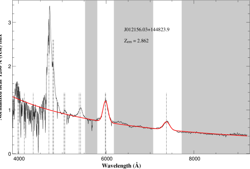
We derive a redshift of the quasar using C iv and C iii]  emission lines in order to be able to estimate the position of these lines and to avoid them when fitting the power-law. This is therefore not an attempt to derive the exact systemic quasar redshift which is known to be shifted compared to the C iv-C iii] redshift (e.g. Vanden Berk et al., 2001; Hennawi & Prochaska, 2007).

Here we assume that the continuum redwards to the Lyman-$\alpha$ emission line can be described as the sum of a power-law component and a gaussian function for each of C iv and C iii]  emission lines. The redshift and the power-law component are estimated as follows (see Fig. 1 for a typical example at $z_{em}=2.862$):

1. After convolving the whole spectrum with a gaussian filter of fixed FWHM = $250\ {\rm km}\,{\rm s}^{-1}$, the position where the flux is maximum is associated to the QSO Lyman-$\alpha$ emission line. This gives a first rough estimate of the redshift, $z_{1}$.

2. The average of the positions of the maximum flux within a window of 100 Å in the rest frame of the quasar (at $z=z_{1}$) around C iv and C iii] emission lines provides a second redshift estimate, $z_{2}$. This redshift should be more accurate than $z_{1}$ because the peak of the Lyman-$\alpha$ emission is a poor estimate of the redshift due to the presence of the Lyman-$\alpha$ forest and the blending with N v$\lambda$1240.

3. A power-law component of the continuum is fitted using windows devoided of emission lines between 1430-1500 Å, 1600-1830 Å and 2000-2500 Å  in the rest-frame (see grey windows in Fig. 1). This component is subtracted from the spectrum.

4. Finally, C iv and C iii] emission lines are simultaneously fitted with gaussian functions. The width and amplitude are independant parameters, but the two gaussian functions are bound to have the same redshift, $z_{3}$.

The red line in Fig. 1 is the sum of the power law and the two emission lines. The extrapolation of the power-law component bluewards to the Lyman-$\alpha$ emission provides a first estimate of the quasar continuum (red line in Fig. 1).

2.3 Principal Component Analysis

We summarize here the main steps of the method as described in Francis et al. (1992) and Suzuki et al. (2005).

2.3.1 Reconstructed continuum

A representative sample of quasar spectra at the redshift of interest must be gathered for which it is possible to define a true continuum, $q(\lambda)$, e.g. unspoiled by intervening absorption. S05 used HST spectra at $z\ \leq 1$ because the IGM is sparse at these redshift and thus the continuum can be easily interpolated above absorption lines. The sample of SDSS-DR7 quasars we used has a mean emission redshift of $z\sim 2.9$ and is defined in Section 3. We derived the true continuum, $q(\lambda)$, by eye and used these fitted quasar continua in the following.

A covariance matrix $V$ is first calculated for the N QSOs in the sample as:

$$\mbox{\boldmath$V$}(\lambda_{\rm m},\lambda_{\rm n})=\frac{1}{N-1}\sum_{\rm i=1}^{\rm N}\left(q_{\rm i}(\lambda_{\rm m})-\mu(\lambda_{\rm m})\right)\left(q_{\rm i}(\lambda_{\rm n})-\mu(\lambda_{\rm n})\right).$$ (1)

where $\mu(\lambda)=1/N\sum_{\rm i=1}^{\rm N}q_{\rm i}(\lambda)$ is the mean quasar continuum.

The principal components are found by decomposing the covariance matrix $V$ into the product of the orthonormal matrix $P$ which is composed of eigenvectors, and the diagonal matrix $\Lambda$ containing the eigenvalues:

$$\mbox{\boldmath$V$}=\mbox{\boldmath$P$}^{-1}\times\mbox{\boldmath$\Lambda$}\times\mbox{\boldmath$P$}.$$ (2)

We call the eigenvectors (i.e. the columns of the matrix $P$) the principal components, $\xi_{\rm j}$. The principal components are ordered according to the amount of variance in the training set they can accommodate, such that the first principal component is the eigenvector which has the largest eigenvalue.

The distribution of the weights, $c_{\rm j}$, of the jth principal component in Eq. 4 is found from the distribution of the $c_{\rm ij}$ for all $i=1..N$ QSOs of the sample:

$$c_{\rm ij}=\int_{1020{\rm\AA}}^{2000{\rm\AA}}(q_{\rm i}(\lambda)-\mu(\lambda))\;\xi_{\rm j}(\lambda)\;d\lambda.$$ (3)

Note that the upper limit of the integration is larger here compared to S05. This is discussed further in Section 3. A mock continuum can now be constructed using Eq. 4 over the rest frame wavelength range of the spectra in the sample.

$$q(\lambda)\sim\mu(\lambda)+\sum_{\rm j=1}^{\rm m}c_{\rm j}\;\xi_{\rm j}(\lambda),$$ (4)

2.3.2 Predicted continuum

The goal is to quantify the relationship between the red and blue sides of the spectra in the sample. The first $m$ principal components $\xi_{\rm j}(\lambda)$ and their weights, $c_{\rm ij}$, are derived as described above, using the whole rest wavelength range, 1020 to 2000 Å. Another set of $m$ principal components, $\zeta_{\rm j}(\lambda)$ and their weights, $d_{\rm ij}$, are defined using only the red rest wavelength range, 1216 to 2000 Å. Finally, we solve linear equations to find a projection matrix relating $c_{\rm ij}$ and $d_{\rm ij}$. Weights can be written in the $N\times m$ matrix form $C$ $=c_{\rm ij}$ and similarly for $D$. We then use singular value decomposition techniques (Press et al., 1992) to derive the $m\times m$ projection matrix $X$ $=x_{\rm ij}$ translating weights found with the red side only into the weights for the whole spectrum:

$$\mbox{\boldmath$C$}=\mbox{\boldmath$D$}\cdot\mbox{\boldmath$X$}.$$ (5)

Once matrix $X$ is known, we can estimate the continuum over the Lyman-$\alpha$ forest for any quasar spectrum from the red part of the spectrum. We proceed in three steps. The weights for the red spectrum are found,

$$b_{\rm j}=\int_{1216{\rm\AA}}^{2000{\rm\AA}}(q(\lambda)-\mu(\lambda))\;\zeta_{\rm j}(\lambda)\;d\lambda.$$ (6)

The weights from the red side $b_{\rm j}$ are translated to weights for the whole spectrum, using

$$a_{\rm j}=\sum_{\rm k=1}^{\rm m}b_{\rm k}\;x_{\rm kj}.$$ (7)

Then the continuum for the whole spectrum is built as:

$$p(\lambda)=\mu(\lambda)+\sum_{\rm j=1}^{\rm m}a_{\rm j}\;\xi_{\rm j}(\lambda).$$ (8)

3 New PCA continuum at $z\sim 3$

The eigenvectors and coefficients as derived by S05, at low redshift, have been used to generate mock spectra in order to test different analysis at high redshift (Dall’Aglio et al., 2008; Kirkman et al., 2005). To our knowledge, one attempt has also been made to derive a similar decomposition at high redshift using SDSS spectra (McDonald et al., 2005). The latter authors comment that this continuum determination is robust enough to infer the mean flux evolution, but unstable as far as the Lyman-$\alpha$ power spectrum is concerned. However the decomposition is not performed on a well controlled training sample as in S05 and in the present work (see below), therefore, they do not provide a projection matrix. The analysis performed by Yip et al. (2004) is closer to our purpose. They applied a PCA to the 16,707 Sloan Digital Sky Survey DR1 quasar spectra (0.08 $<z<$ 5.41) and reported that the spectral classification depends on redshift and luminosity. No compact set of eigenspectra succeeds in describing the variations observed over the whole redshift range. Besides, it seems that there is a differential evolution with redshift of the coefficients. Since these authors are interested in the quasar continuum only, they do not try to recover the exact continuum over the Lyman-$\alpha$ forest, and consider only the observed flux (that is continuum plus absorption).

Due to the large difference of redshift between the quasars used in S05 and those involved in any Lyman-$\alpha$ forest study using SDSS spectra, one may wonder if there is any evolution in the continuum of quasars or any change in the correlation between the shapes of the continuum over the forest and redwards to the Lyman-$\alpha$ emission compared to what is found by S05. Deriving new components at redshift 3 should answer this question.

The other motivation for this work is to provide principal components and distributions of coefficients over a larger wavelength coverage than in previous studies: the S05 matrix allows to generate continua from Lyman-$\beta$ to C iv emission lines while in the present work we will extend the wavelength coverage beyond the C iii]  emission line (until 2000 Å in the restframe). This should in principle facilitate the extrapolation in the blue.

3.1 Deriving new principal components from a sub-sample of $z\sim 3$ SDSS-DR7 quasar spectra

The difficulty of this analysis is to estimate the continuum in the Lyman-$\alpha$ forest, where absorption can be neither neglected nor easily removed because of the low resolution of SDSS spectra. In particular it would be very difficult to define the true continuum automatically.

We first selected spectra with a signal-to-noise ratio per pixel greater than 14 redwards to the Lyman-$\alpha$ emission (the SNR is computed around 1280 Å in the restframe). We require the redshift of the quasars to be greater than 2.82 and lower than 3.00. The lower limit is chosen as such for two reasons: the Lyman-$\alpha$ forest has to be complete ($z>2.7$) and we noticed that there is some issues with the flux calibration at the very blue end of the SDSS spectra so that we would like to avoid this part of the spectrum. To illustrate these problems and estimate the exact wavelength at which to start the study, we have selected spectra where a damped Lyman-$\alpha$ system (DLA) is observed with aborption redshift greater than 3.7 and with a column density $N$(H i) $\geq 10^{20.5}{\rm cm}^{-2}$ (the list is available in Noterdaeme et al., 2009). 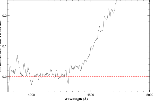In these spectra, and due to the presence of the DLA, the flux is expected to be equal to zero for $\lambda_{\rm obs}\leq 4280$ Å. When stacking the selected lines of sight (Fig. 2), we note instead that the flux increases for wavelength lower than 4000 Å. The difference with zero is as high as 0.05 for a normalized spectrum, meaning that this part of the spectrum should probably not be used for the analysis. Since the study of the forest is usually limited to beyond the O vi emission line ($\lambda_{\rm rest}>1050$ Å), the minimum emission redshift will be 2.82. The upper limit is a compromise between the number of spectra needed for the analysis and our ability to estimate confidently a continuum by eye: it has been set to $z=3$. BAL quasars, lines of sight containing a DLA or any spectrum for which fitting a continuum is too risky because of missing pixels or reduction issues are removed from the analysis. The SDSS spectra are observed with two cameras, one for the blue and one for the red part of the spectrum and we were concerned about the presence of a possible discontinuity or break at the merging point. We have avoided any spectra possibly affected by this. When applying all those constraints, 78 spectra remain in the training set (Table 1).

QSO	$z_{\rm em}$	$m_{\rm g}$	SNR	SNR	QSO	$z_{\rm em}$	$m_{\rm g}$	SNR	SNR
			(forest)	(red)				(forest)	(red)
J090439.50+221050.3	2.823	18.23	12.14	17.62	J134826.65+290623.0	2.822	19.21	13.71	18.16
J123549.46+591027.0	2.820	17.05	21.16	28.86	J221936.37+002434.0	2.850	18.98	10.73	17.04
J020950.71-000506.4	2.848	17.03	19.00	29.13	J103249.88+054118.3	2.841	17.37	19.05	28.40
J121723.67+254910.5	2.834	18.50	10.55	14.09	J143455.38+035030.9	2.845	18.35	9.38	14.94
J093434.74+543109.4	2.836	18.81	9.22	14.75	J143823.51+083128.6	2.834	18.39	10.82	17.35
J113429.70-011153.6	2.860	19.37	8.10	14.09	J162331.14+481842.1	2.830	17.99	12.94	19.75
J102734.13+183427.5	2.832	18.03	28.31	34.12	J125251.95+202405.0	2.877	18.80	10.47	15.03
J084948.98+275638.7	2.845	17.96	14.99	21.35	J131114.90-023045.5	2.860	18.51	13.07	16.97
J123503.01+441118.2	2.845	18.54	8.18	14.25	J124652.81-081312.9	2.854	18.27	18.04	30.13
J094152.90+621705.5	2.862	19.48	11.07	15.44	J012156.03+144823.9	2.869	17.22	25.65	31.14
J134450.86+191843.4	2.860	19.68	11.20	14.92	J102832.09-004607.0	2.867	18.14	9.91	15.25
J160843.90+071508.6	2.877	16.80	25.54	35.30	J103000.37+440010.7	2.870	18.99	11.72	16.81
J031522.09-080043.7	2.895	18.42	11.68	18.74	J114218.85+572824.4	2.897	18.82	9.86	15.14
J105236.34+253956.1	2.896	17.85	18.08	23.63	J093207.46+365745.5	2.878	17.70	22.55	27.03
J111033.39-113259.9	2.895	18.17	11.38	17.02	J112857.85+362250.2	2.885	18.04	15.51	20.37
J085733.39+370045.6	2.946	18.94	15.53	22.39	J135044.66+571642.9	2.893	17.45	19.79	27.28
J170144.31+284234.2	2.913	19.28	11.54	18.79	J003311.34-171041.5	2.905	17.97	12.08	20.60
J124754.78+492758.2	2.935	19.13	15.06	22.02	J131440.18+271449.5	2.935	18.68	10.86	14.69
J101539.35+111815.9	2.905	18.57	12.10	16.10	J094442.31+255443.3	2.901	18.59	11.60	16.48
J142950.91+260750.2	2.910	18.40	11.57	16.77	J093643.51+292713.6	2.922	18.10	13.79	17.98
J163842.52+360213.8	2.910	19.36	13.18	19.67	J120322.71+403310.1	2.915	19.14	11.10	15.88
J012305.58+063047.2	2.923	19.07	11.99	16.07	J135225.88+293830.4	2.915	18.43	9.32	14.35
J102807.74+172956.8	2.926	18.11	30.59	41.45	J100808.27+285214.6	2.921	18.53	10.11	14.56
J130554.81+184904.9	2.925	18.27	13.79	21.28	J152119.68-004818.7	2.934	17.93	19.39	25.50
J075326.11+403038.6	2.929	17.92	13.80	20.90	J103928.63+253345.4	2.933	18.69	11.40	14.90
J004129.80+241702.1	2.934	19.32	12.94	18.51	J223927.69+230018.0	2.928	18.41	14.47	19.71
J160441.47+164538.3	2.932	16.91	29.71	38.00	J102025.27+334633.4	2.930	18.21	13.54	18.48
J120753.79+325747.4	2.945	18.89	9.92	14.25	J141442.96+193523.5	2.946	18.32	11.46	15.61
J131212.60+001129.7	2.945	19.27	9.76	16.18	J082257.04+070104.3	2.940	18.65	11.05	15.02
J111038.63+483115.6	2.953	16.79	26.22	33.02	J130337.21+194926.7	2.953	17.84	16.79	22.49
J104253.44-001300.8	2.953	18.87	11.98	17.11	J134811.76+281801.8	2.966	17.57	26.29	39.35
J091546.67+054942.7	2.967	18.40	9.35	14.37	J125708.23+191857.2	2.970	18.61	19.54	27.02
J113559.41+422004.4	2.953	18.57	9.35	14.38	J090423.37+130920.7	2.968	17.59	22.46	30.62
J120331.29+152254.7	2.976	16.99	24.55	32.71	J142807.87+162634.3	2.977	18.32	12.90	18.00
J013829.75+224558.9	2.987	19.11	10.03	14.84	J085959.14+020519.7	2.970	18.45	10.52	15.43
J132255.66+391207.9	2.984	17.76	19.45	25.44	J120006.25+312630.8	2.978	16.62	29.81	34.04
J132321.24+250027.4	2.980	18.00	11.72	15.97	J125419.07+362750.4	2.980	18.51	13.68	17.43
J074313.86+28442.3	2.975	19.45	12.31	14.84	J143912.34+295448.0	2.992	17.65	17.65	24.10
J075710.36+362301.5	2.990	18.79	11.63	15.36	J224154.38+000102.1	2.998	19.12	9.57	14.26

Table 1: List of SDSS-DR7 quasars used to define the correlation matrix and the eigenvectors at $z\sim 3$

Figure 2: Result of the stacking of SDSS-DR7 spectra with a damped Lyman-$\alpha$ system at an absorption redshift larger than 3.7 and a column density $N$(H i) $\geq 10^{20.5}{\rm cm}^{2}$. The spectra are normalized to 1 near 1280 Å (in the quasar restframe). Due to the presence of the DLA, the flux is expected to be equal to zero at observed wavelength smaller than 4280 Å. It can be seen from the figure that this is not the case in the very blue of the spectrum ($\lambda_{\rm obs}\leq$ 4000 Å ) where the mean flux is increasing. Consequently, pixels at wavelengths below 4000Å are not used in this analysis.

Figure 3: Spectrum and continuum of the quasar SDSS J134826.65+290623.0. This quasar belongs to the sample of SDSS $z\sim 3$ quasars that is used to derive the Principal Component Analysis eigenvectors (Section 3). Our estimate of the continuum is shown with the thick red line and a zoom in the Lyman-$\alpha$ forest region is shown in the inset.

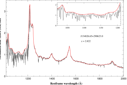
Once the training set is defined, spectra are smoothed and the continuum is ”hand-fitted”. Redwards to the Lyman-$\alpha$ emission line, we follow the different emission lines and ignore isolated absorption lines. In the Lyman-$\alpha$ forest, the continuum cannot be uniquely defined. We assume that the continuum has a smooth shape, that it roughly follows the peaks of the spectrum, and that the blending of lines at the SDSS resolution is large. Points are placed around the peaks of the flux, and a spline interpolation is used to connect them. After a first try, we minimize the number of points used and we check that the continuum is indeed located above blends of lines, but at about the level of ’flat’ regions. A typical example is given in Fig. 3. Note that with this procedure, we de facto take into account that the chosen points can be affected by some absorption. 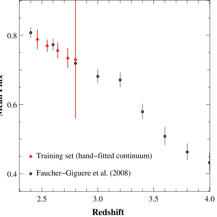To check that this is indeed the case, the spectra are then rebinned with 0.5 Å restframe pixels and the mean flux evolution is computed and compared to Faucher-Giguère et al. (2008) measurements from high and medium resolution and high signal-to-noise spectra. Both estimates are in agreement giving us confidence in our hand-fitted continua (Fig. 4).

Figure 4: The mean flux evolution in the training set (with redshift bins of size $\Delta z=0.1$; red triangles) is compared to FG08 measurements from high resolution and high signal-to-noise spectra (black circles). The continuum of the 78 SDSS spectra in the training set have been fitted by hand using spline interpolation. Error bars from our measurements have been computed by bootstrapping pixels of our sample. Both measurements are consistent, making us confident in our continuum estimate.

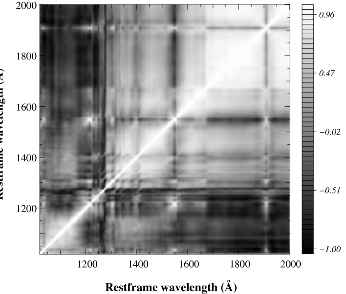
The procedure described in Section 2.3 is then performed and the correlation matrix is computed and displayed in Fig. 5. In agreement with S05, a moderate correlation (0.3-0.6) is found between the shape of the continuum in the forest and the region between Lyman-$\alpha$ and C iv emission lines. Thanks to the larger restframe wavelength coverage of this study, a moderate anti-correlation (from -0.6 to -0.4) between the shape of the continuum in the forest and in the region between C iv and C iii] emission lines is found. S05 noticed that a PCA continuum has the good shape in the forest but that the amplitude of the power-law component is unstable. The anti-correlation in that extra-part of the continuum may improve the stability of the prediction of the amplitude of the continuum in the forest. This is discussed in more details in Section 3.2.1.

Figure 5: Correlation matrix computed with the training set. A moderate correlation (0.3-0.6) is found between the shape of the continuum in the Lyman-$\alpha$ forest (1020 $\leq\lambda\leq$1210 Å) and in the region between Lyman-$\alpha$ and C iv emission lines (1216 $\leq\lambda\leq$1600 Å), in agreement with S05. We note also a moderate anti-correlation (from -0.6 to -0.4) between the continuum in the Lyman-$\alpha$ forest and the region further to C iv emission line.

Figure 6: The solid black (resp. dashed red) line is the mean continuum of quasars at $z=3$ (resp. $z\leq 1$, S05). The wavelength coverage at $z=3$ corresponds to SDSS spectra and is larger than at $z\leq 1$. The main difference between the two mean spectra is seen in the amplitude of emission lines. The composite spectrum from Vanden Berk et al. (2001) computed from 2,200 SDSS spectra (dash-dot blue line) is in good agreement with our mean continuum. The difference in the Lyman-$\alpha$ forest is due to the fact that Vanden Berk et al. (2001) did not try to avoid the absorption from the IGM. A small shift in the position of emission lines can be noticed: this is because Vanden Berk et al. (2001) have used the Mg ii line as a reference to compute the redshift whereas we have used the C iv and C iii] lines.

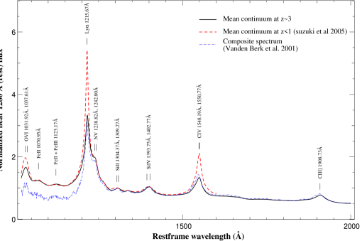
The mean continuum is shown in Fig. 6 together with the mean continuum of S05 ($z\leq 1$) and the composite spectrum derived by Vanden Berk et al. (2001). In the wavelength range of interest here, quasars contributing to the Vanden Berk et al. (2001) composite cover a redshift range from 2.13 to 4.789 for the Lyman-$\alpha$ region and from 1.5 to 4.789 for C iv. Our mean continuum is in excellent agreement redwards to the Lyman-$\alpha$ emission line with the Vanden Berk et al. (2001) composite. The discrepancy in the blue is simply due to the absorption in the Lyman-$\alpha$ forest that Vanden Berk et al. (2001) did not try to remove. When comparing to S05, one can see that the amplitude of C iv, Lyman-$\alpha$ and Lyman-$\beta$ emission lines relative to the continuum are less important in the SDSS spectra. While the determination of the C iv emission is relatively straightforward, the presence of absorption at the position of the Lyman-$\beta$ emission line and in the blue wing of the Lyman-$\alpha$ emission line makes the continuum difficult to estimate. Thus, the main and robust difference between the mean continua in SDSS and HST spectra is the variation of the C iv equivalent width. Such an evolution of the QSO emission line equivalent widths has been noted for long (Baldwin, 1977) and has also been reported by Zheng et al. (1997). The later authors used 101 HST spectra to compute a low-$z$ composite spectrum (90% of the quasars had a redshift lower than 1.5) and compared it to the Francis et al. (1991) composite ($z\sim 3$). This evolution is probably related to the quasar luminosity. Note that no evolution is found by Fan (2009) from $z\sim 2$ to $z>6$.

Figure 7: First ten principal components of a Principal Component Analysis applied to (i) $z\sim 3$ SDSS quasar spectra (black solid lines) over the range 1020$-$2000 Å and to (ii) $z\leq 1$ HST quasar spectra (S05, red dashed lines) over the range 1020$-$1600 Å . The distributions of the coefficient associated to each component are shown in the right panel (grey histogram) together with their fit with a Gaussian (except for the first component for which the distribution is log-normal; thick black line).

Figure 8: First ten principal components obtained from a Principal Component Analysis of the QSO spectrum redwards to the Lyman-$\alpha$ emission line, for (i) the $z\sim 3$ SDSS quasar spectra (black solid lines) and (ii) the $z\leq 1$ HST quasar spectra (S05, red dashed lines). The distributions of the coefficient associated to each component are shown in the right panels (grey histogram) together with a Gaussian fit (except for the first component for which the distribution is log-normal; thick black line).

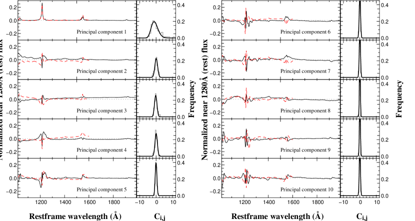
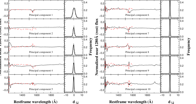
Further, the first ten eigenvectors are displayed in Fig. 7 when derived from the full wavelength coverage and in Fig. 8 when derived from the region redwards to the Lyman-$\alpha$ emission, together with the components provided by S05. The distributions of the coefficients, $c_{\rm i,j}$ and $d_{\rm i,j}$, computed on our sample using Eq. 3, are also shown. The first component looks very similar in the two decompositions and is dominated by the amplitude of the Lyman-$\alpha$ and C iv emission lines. The most important difference with S05 lies in the shape of the distribution of the associated coefficients: in their study, the distribution is Gaussian whereas in ours, this distribution is log-normal. This trend (concerning the eigenvectors and the distributions of coefficients) is in agreement with what has been found by Francis et al. (1992). The discrepancy between the shapes of the coefficient distributions could mean that the S05 sample is more homogeneous than ours in term of amplitude of emission lines.
The second component is dominated by the continuum slope and it seems that there is a difference between what is found here and in S05 which seems to be somewhat compensated by the difference in the third component. Other components show small differences but they are less pronounced and the coefficient distributions are very similar.
To estimate more quantitatively the similarity of the low and high redshift sets of eigenspectra, we follow Yip et al. (2004), and compute the sum of the projection operators of each set of eigenvectors $|\xi_{\rm j}>$:

$$\mathbf{\Xi}=\sum_{\rm j=1,m}|\xi_{\rm j}><\xi_{\rm j}|\ ,$$ (9)

and then the trace of the products of the projection operators:

$$Tr(\mathbf{\Xi_{z=3}\Xi_{S05}\Xi_{z=3}}) = D\ ,$$ (10)

where D will be the common dimension of both sets. The two sets are disjoint if the trace is zero. If the basis are completely alike, $D$ should be equal to their dimension, therefore $D=10$ in our case. To compute this number, we cut our eigenspectra at 1600 Å (rest) and we find $D=7.6$. This means that the two decompositions are similar but not exactly the same, confirming the slight evolution of the decomposition with redshift.

We provide in an electronic form the first 10 eigenvectors of the PCA. The distributions of associated coefficients are very close to gaussian functions, except for the first coefficient, the distribution of which is fitted with a log-normal distribution. Their characteristics are listed in Table 2.

Component $j$	$c_{i,j}$ distribution
	$\mu$	$\sigma_{\mu}$	$\sigma$	$\sigma_{\sigma}$
1	2.645	0.008	0.145	0.006
2	0.090	0.033	0.845	0.033
3	-0.220	0.019	0.745	0.019
4	0.044	0.031	0.717	0.031
5	-0.029	0.003	0.496	0.004
6	0.028	0.002	0.386	0.003
7	0.020	0.003	0.363	0.004
8	0.018	0.002	0.258	0.008
9	0.034	0.002	0.284	0.006
10	0.008	0.001	0.336	0.001

Table 2: Parameters of the fits to the distributions of weights, $c_{\rm i,j}$, for the first ten principal components. The distributions have been fitted with gaussian functions, except for the distribution of the first coefficient which has been fitted with a lognormal function.

3.2 Quality of the predicted continuum

The decomposition of the quasar emission investigated at $z\leq 1$ by S05 with HST spectra and at $z\sim 3$ in this paper with SDSS spectra yield two similar but different basis of eigenvectors, as shown in the previous Section. One would like to know if the larger wavelength coverage of our eigenvectors provides any advantage and how far the new determination is required to reproduce the correct quasar continuum at $z\sim 3$. In other words, is the prediction of quasar continuum at $z\sim 3$ better if one uses the new PCA eigenvectors derived in this paper ? To answer this question, we apply three tests to the predicted continua.

3.2.1 Error on the predicted PCA continuum in the Lyman-$\alpha$ forest

In order to estimate the difference between the true and predicted continuum in the Lyman-$\alpha$ forest, a set of eigenvectors and a projection matrix are derived using 77 spectra of the training set (out of 78) and the continuum over the Lyman-$\alpha$ forest for the remaining quasar is estimated using these parameters and following the method described in Section 2.3. That procedure is repeated on each of the 78 spectra in the training set.
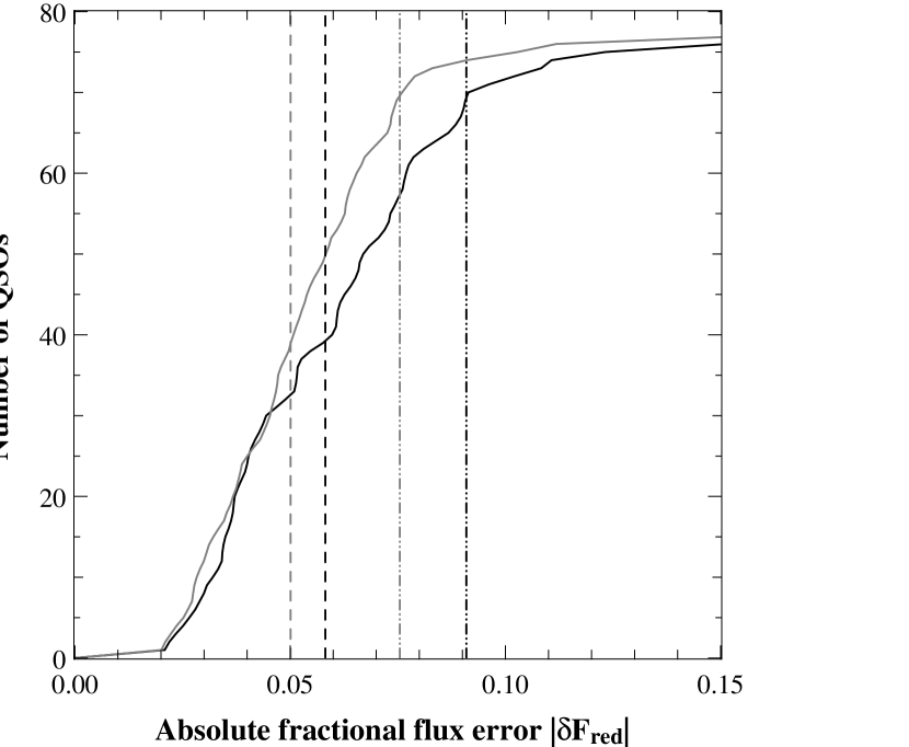
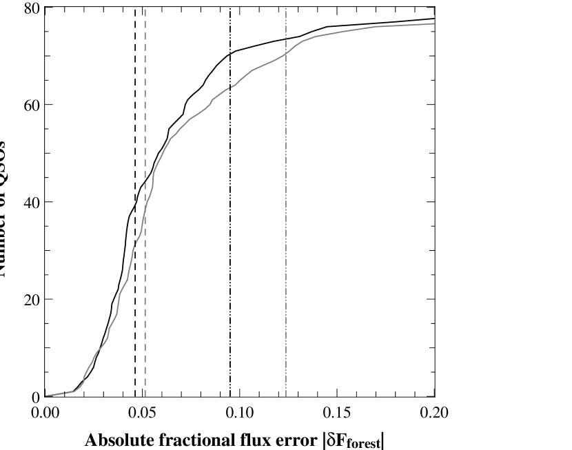
Following S05, we estimate for each spectrum, the absolute fractional flux error $\left|\delta F\right|$, defined as follows,

$$\left|\delta F\right|=\left.\int_{\lambda_{1}}^{\lambda_{2}}\left|\frac{p(\lambda)-q(\lambda)}{q(\lambda)}\right|d\lambda\right/\int_{\lambda_{1}}^{\lambda_{2}}d\lambda,$$ (11)

where $p$ and $q$ are, respectively, the predicted and real continua.

This has been computed over the restframe wavelength ranges, 1050-1170 Å in the forest, and 1280-2000 Å (or 1280-1600 Å) in the red. The cumulative distributions of the absolute fractional flux errors are plotted in Fig. 9 (in the red) and Fig. 10 (in the forest) using two different wavelength coverages (black line for 2000 Å and grey line for 1600 Å).
In the red, the median error is 5.8% and 5% using, respectively, the 2000 Å and the 1600 Å decompositions (Fig. 9, black dashed and grey dotted vertical lines respectively) and the 90^th percentile error with the 2000 Å decomposition is larger than the error using the 1600 Å set of eigenspectra. This indicates simply that the range up to 1600 Å  is easier to fit.

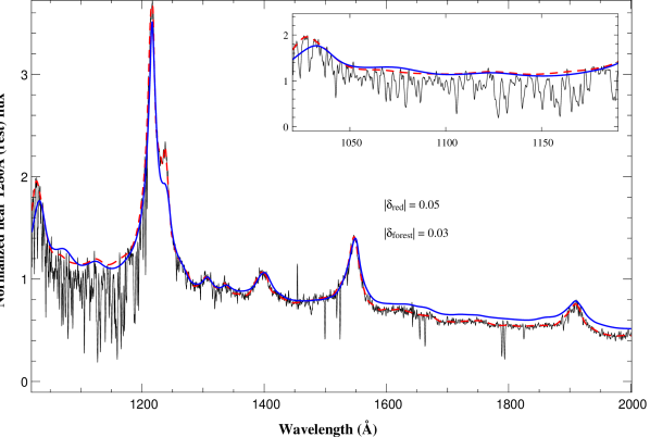
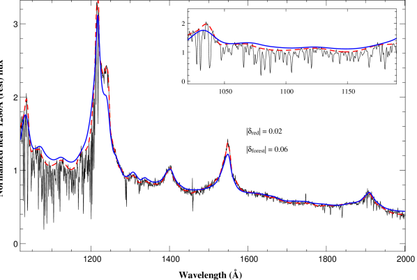
The important result is that the opposite trend is observed in the forest (Fig. 10): median values (around 5%) are very close for the two wavelength coverages (black and grey dashed vertical lines) whereas the 90^th percentiles are different (black and grey dot-dot-dash vertical lines) with 9.5% and 12.4% errors for, respectively, the 2000 and 1600 Å decompositions. This means that using the full coverage reduces the number of outliers with more than 12% error in the Lyman-$\alpha$ forest. Errors in S05 are similar to those we find here but, by using the 2000Å decomposition, outliers are less frequent than in the previous study. To illustrate what those numbers mean on the continuum level, examples of spectra with their predicted continua are displayed in Fig. 11.

Figure 9: Cumulative distributions of the absolute fractional flux error (Eq. 11) redwards to the Lyman-$\alpha$ emission line when predicting spectra with PCA decompositions over a wavelength range extending up to 2000 Å (black solid line) or up to 1600 Å (grey solid line). Median values are similar for the two estimates (black and grey dashed vertical lines respectively). The 90^th percentile from the 1600 Å decomposition (dash-dot-dot grey vertical line) is lower than one for the 2000 Å decomposition (dash-dot-dot black vertical line).

Figure 10: Same as Fig. 9 for the cumulative distributions of the absolute fractional flux error (Eq. 11) in the Lyman-$\alpha$  forest.

Figure 11: Example of a spectrum with (i) a large absolute fractional flux error in the red and a small error in the forest (upper panel) and (ii) a large absolute fractional flux error in the forest and a small error in the red (lower panel). The hand-fitted continuum is the red dashed line and the predicted one is the solid blue line.

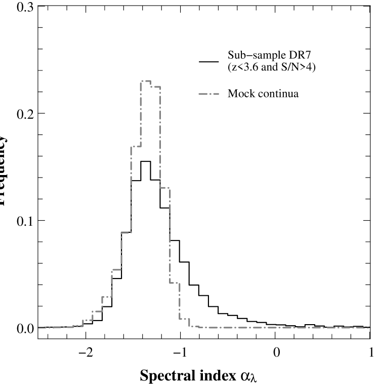
3.2.2 Distribution of spectral indices

We can also compare the characteristics of mock continua generated from the set of computed eigenvectors and the distribution of weights $c_{\rm ij}$ given in Table 2 with those of real spectra from SDSS-DR7. For this, we have fitted in the same way a power-law to mock continua and to SDSS-DR7 spectra (see Section 4.2 for more details). The normalized (sum equal 1) distributions of the derived power-law index are displayed in Fig. 12. The distribution from mock spectra is more peaked than the one from SDSS spectra but is centered around the same value. This behavior is expected because the PCA gives us a mean description of the whole quasar population.

Figure 12: Distribution of spectral indices derived by fitting a power-law to mock continua generated using the principal components and the distributions of coefficients $c_{\rm ij}$ derived from our SDSS-DR7 subsample (grey histogram) compared to the spectral index distribution obtained from fitting SDSS-DR7 spectra (black histogram).

3.2.3 Prediction of the continuum: fitting coefficients versus using the projection matrix

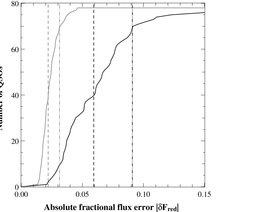
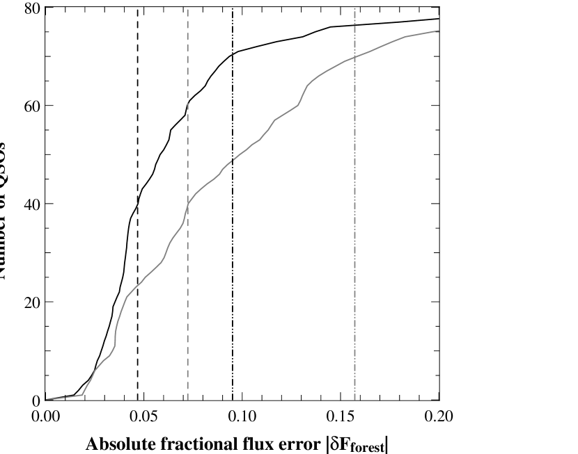
Our goal is to estimate the quasar continuum over the Lyman-$\alpha$ forest. For this, we estimate first the weights of the red part of the spectrum in the basis obtained from PCA of the red part of the spectra. We then multiply these weights by the projection matrix (see Eq. 5) to compute the weights to be used in the basis obtained from the overwhole spectrum. This gives us the spectrum reconstructed in the whole wavelength range (method 1). One may be tempted to directly use the coefficients obtained from the red part of the spectrum as representative of the whole spectrum just replacing the eigenvectors obtained from the red part by those obtained from the full wavelength coverage (method 2). To test how useful the projection is, both methods have been used to predict the continuum and the distributions of absolute fractional flux error (Eq. 11) have been computed and are displayed in Fig. 13 and Fig. 14.

When using method 2, and not surprinsigly, the red part of the spectrum is very well fitted with a median error less than 2.5% (Fig. 13, dashed grey line) and method 1 (projection) leads to larger errors (dashed black line in Fig. 13, median error $\sim$6%). In the forest, the trend is opposite with a median error less than 5% when method 1 is applied (Fig. 14, dashed black line) and more than 7% when method 2 is applied (dashed grey line). In addition, with method 2, 10% of the spectra have more than 15% error (dot-dot-dash grey line) for only one percent with method 1. It is therefore apparent that the projection matrix should be used.

Figure 13: Cumulative distributions of the absolute fractional flux error in the red part of the spectra in the training set: (i) when the weights used to reconstruct the spectrum are those obtained from the red part of the spectrum (method 1, grey line); (ii) when the projection matrix is used (method 2, black lines). Median values are displayed (dashed vertical lines) together with 90^th percentiles (dot-dot-dashed vertical lines).

Figure 14: Same as Fig. 13 in the Lyman-$\alpha$ forest. Errors are less when the projection matrix is used (method 2, black line, see Text). The number of outliers (spectra with large errors) is much smaller in that case.

4 Evolution of the mean flux

An important application of the quasar continuum estimate over the Lyman-$\alpha$ forest wavelength range is the determination of the redshift evolution of the mean flux in the IGM. Numerous authors have performed this measurement using high and/or intermediate spectral resolution data (e.g. Songaila, 2004; Bernardi et al., 2003; Dall’Aglio et al., 2008, 2009; Faucher-Giguère et al., 2008). The evolution is smooth except for a possible bump at $z\sim 3.2$ which could be related to the He ii reionization (Schaye et al. 2000), although this is not the only possible explanation (Faucher-Giguère et al., 2008). In this Section we reinvestigate this issue applying the method developped in Section 3.

4.1 Comparison with B03

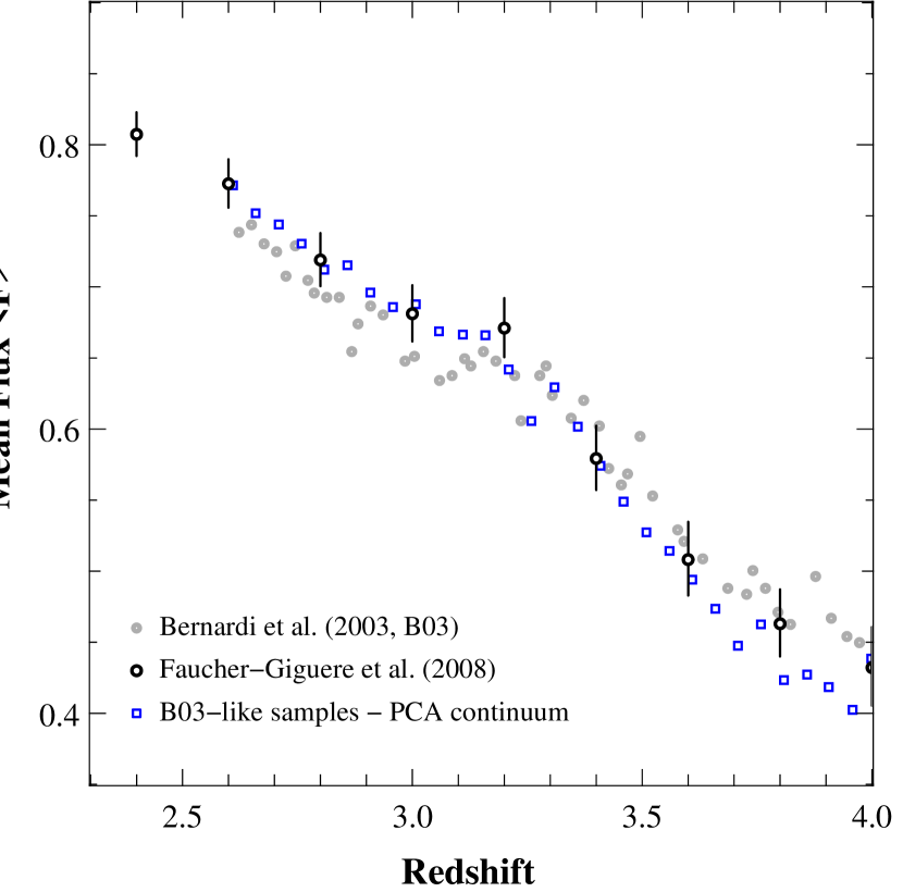
We first would like to check if we can recover the Bernardi et al. (2003) results. The sample used in the Bernardi et al. (2003) study is a sub-sample of SDSS-DR7 containing all the spectra observed up to the end of 2001 (corresponding to a modified Julian day $mjd=52274$). Some selection is applied to remove most prominent BALs and DLAs. These objects are not clearly defined in Bernardi et al. (2003) so that we have to apply our own selection. We avoid all BALs and DLAs as defined by Noterdaeme et al. (2009). Our final sample has 837 QSOs when B03 had 1041. The comparison to B03 is shown in Fig. 15 (left hand-side panel) for power-law (triangles) and PCA (squares) estimates of the continuum. Shown in the figure as well are the Faucher-Giguère et al. (2008) results. As expected (see next Section), the power-law estimate is lower at $z<3$ than other estimates. The evolutions found by us and B03 are in agreement and a departure from a smooth evolution is seen at $z\sim 3.2$.

We have randomly drawn from SDSS-DR7 a large number (500) of samples identical in size and redshift distribution to the B03 sample. For each sample, we derived the mean flux observed at each redshift and calculated the mean over the 500 samples. The result is shown in Fig. 15 (right hand-side panel). The feature at $z\sim 3.2$ is still seen and could be a ”bump” or a break in the evolution. Note that, as emphasized by Faucher-Giguère et al. (2008), a bump is seen only if one insists on fitting a single power-law.

Figure 15: Left hand-side panel: Mean flux redshift evolution inferred from power-law (red triangles) and PCA (blue squares) estimates of the continuum using a sample similar to Bernardi et al. (2003); the mean flux evolutions reported by Bernardi et al. (2003) and Faucher-Giguère et al. (2008) are shown as, respectively, grey points and black open circles. Our measurements are consistent with B03 and FG08 results. In particular, a departure from a smooth evolution is seen at $z\sim 3.2$. Right hand-side panel: 500 samples are randomly drawn from the SDSS-DR7 (similar in size and redshift distribution to the B03 sample) and the mean flux evolution for each sample is then computed. The average of these measurements is displayed (PCA continuum, blue squares) and is in excellent agreement with Faucher-Giguère et al. (2008) measurement.

4.2 Redshift evolution of the mean flux in the IGM using SDSS-DR7

Continua of SDSS-DR7 spectra have been fitted using the two different methods we have described previously. We derive a power-law and a PCA (using our and S05 sets of eigenspectra) continua. We restrict our study to spectra with a signal-to-noise ratio greater than 8 around 1280 Å in the restframe to avoid instabilities in the fit of the power-law. We restrict the analysis to quasars with redshifts larger than $z>2.45$ to avoid the blue end of the spectra.

Lines of sight containing damped Lyman-$\alpha$ systems (DLAs) have been removed following the lists provided by Noterdaeme et al. (2009) and Prochaska et al. (2005). Broad absorption line quasars (BALs) flagged by Shen et al. (2010) have been avoided as well. After this selection, we are left with 2,576 quasars. Following Bernardi et al. (2003), we compute the mean flux from the Lyman-$\alpha$ forest between 1080 and 1160 Å in the restframe to avoid the O vi-Lyman-$\beta$ and Lyman-$\alpha$ emission lines.

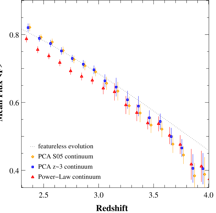
The mean flux in the Lyman-$\alpha$  forest is then computed using three different continua: two PCA continua obtained from S05 principal components and the principal components derived in this work, and a power-law continuum. Fig. 16 shows the redshift evolution of this quantity in redshift bins of size $\Delta z=0.1$. Error bars are computed from a bootstrap resampling. There is apparently no difference in the results when using the two PCA decompositions derived at low ($z\sim 1$) and high ($z\sim 3$) redshifts. The mean flux derived from the power law continuum is systematically smaller at $z<3$. This is expected as, the power-law tends to overestimate the continuum in the forest (see Section 4.3).

It is apparent that there is a change in the evolution of the mean flux at $z\sim 3$ with a steepening of the evolution at large redshift.

Figure 16: Redshift evolution of the mean flux from SDSS DR7 quasar spectra. Three different estimates of the continuum are assumed (Section 2.1): (i) an extrapolation of a power-law fit (see Section 2.2; red triangles); or a prediction (Eq. 4) using the output of a Principal Components Analysis of (ii) SDSS spectra at $z\sim 3$ as described in Section 3 (blue squares) or of (iii) HST spectra at $z\leq 1$ (S05; orange diamonds). Error bars are computed from bootstrapping and are at the 3$\sigma$ level. A change in the evolution can be noticed at $z\sim 3$ in the sense of a steeper slope at high redshift. A featureless evolution (fitted from $z\leq 3$ points using $z\sim 3$ PCA measurement) is shown for guidance.

To estimate what kind of feature we are able to recover with our procedure, we construct in the following DR7-like samples of simulated intermediate resolution quasar spectra probing an IGM with a mean flux evolution as seen in the high resolution data and test if we can recover this evolution by applying our procedures.

4.3 Detectability of the bump with DR7

In order to test the detectability of a feature equivalent to the bump seen at $z\sim 3.2$ by Faucher-Giguère et al. (2008), we performed simulations of this effect and its measurement with mock spectra.

4.3.1 Mock spectra

We want to simulate the Lyman-$\alpha$ forest that will give a mean flux redshift evolution similar to what is seen in high resolution data. This evolution was fitted by Faucher-Giguère et al. (2008) as:

$$F(z)=e^{-A(1+z)^{B}-Ce^{{-\frac{[(1+z)-D]^{2}}{2E^{2}}}}},$$ (12)

where $A=0.00153$, $B=4.060$, $C=-0.0969$, $D=4.267$ and $E=0.0769$.

We assume that the Lyman-$\alpha$ forest is made up of absorption lines with a column density distribution

$$f_{\rm NHI}=\alpha N_{\rm HI}^{-\beta},$$ (13)

with $\alpha=4.9\times 10^{7}$ and $\beta=1.46$ over the column density range $10^{13}-10^{17}$ cm^-2 and a Doppler parameter distribution given by:

$$\frac{{\rm d}n}{{\rm d}b}=K\frac{b_{\sigma}^{4}}{b^{5}}e^{-\frac{b_{\sigma}^{4}}{b^{4}}},$$ (14)

with $K=6.82$ and $b_{\sigma}=24.09\ {\rm km}\,{\rm s}^{-1}$ (Kim et al., 2001). Therefore the evolution in $F(z)$ is supposed to be due to an evolution in the number of clouds per unit redshift. This is probably oversimplistic because, if any, the feature at $z\sim 3.2$ is claimed to be possibly due to an ionization process but this is probably fine for what we want to estimate.

We first construct the relation which gives at a given redshift the mean flux versus the number of cloud present in a redshift bin of $\Delta z=0.1$. This relation is parametrized by:

$$F_{\rm z}(n_{\rm abs})=a_{z}e^{-\epsilon_{\rm z}n_{\rm abs}},$$ (15)

where $n_{\rm abs}$ is the number of clouds drawn at random from the above population of clouds and $a_{\rm z}$ and $\epsilon_{\rm z}$ are determined by the simulation and depends on redshift.

Combining Eqs. 12 and 15, we then derive at each redshift the actual number of clouds that is needed to reproduce the relation given by Faucher-Giguère et al. (2008). We finally fit the redshift evolution of the number of clouds by a similar function:

$$\frac{dn}{dz}=n_{0}(1+z)^{\gamma}+Ce^{{-\frac{[(1+z)-D]^{2}}{2E^{2}}}}.$$ (16)

Our best fit gives the values $n_{0}=8.281\pm 0.080$ and $\gamma=3.076\pm 0.006$, $C=-121.3\pm 4.5$, $D=4.267\pm 0.003$ and $E=-0.081\pm 0.003$ .

Once the number of clouds per unit redshift is correctly calibrated, we generate 50,000 mock spectra with a uniform emission redshift distribution in the range 2.3-4.5. For a given emission redshift, the number of absorption lines is computed from the line number density and is modulated to introduce Poisson noise. For each absorption line, the column density $N_{\rm HI}$ and the Doppler parameter are randomly chosen following Eq. 13 and Eq. 14. The spectrum is then degraded at the SDSS resolution ($R\sim 1800$) and a PCA continuum is added using 10 principal components and choosing the weights at random within the calculated distributions. The wavelength scale is binned as for SDSS spectra and noise is added following the SDSS g-magnitude distribution.

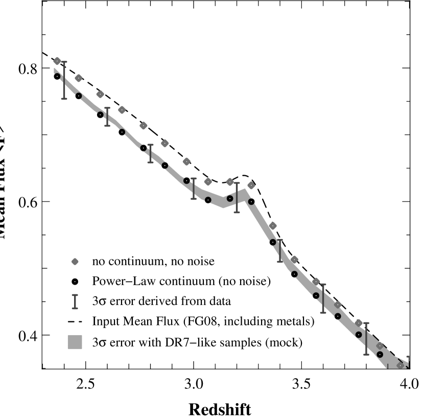
To check the validity of our procedures, the mean flux evolution is computed from spectra with no noise and no continuum added (see Fig. 17). The mean flux evolution recovered by our procedure (grey diamonds) is in excellent agreement with the theoritical input (black dashed line) assumed to follow the evolution as derived by Faucher-Giguère et al. (2008).

4.3.2 Should we detect any feature with DR7?

We compute 100 mock samples with the same number of quasars as the SDSS-DR7 and the same distributions of emission redshift and signal-to-noise ratio. For each sample, we compute the mean flux evolution fitting quasar continuum with a power-law as performed on real data. At each redshift, we compute the scatter in the mean flux derived from these samples. The recovered evolution is shown as black points in Fig. 17, to be compared with the dashed line showing the input assumed for the simulation. As already mentioned, it is apparent that the power-law fit of the QSO continuum underestimates the mean flux. However, the bump at $z\sim 3.2$, introduced in the input, is recovered although slightly smoothed out by the procedure. The errors derived from the simulations are shown as a grey area. They have to be compared with errors expected from the data. The latter are estimated using the errors obtained in SDSS-DR7 from B03-like samples (as in Fig. 15) but scaled by the square root of the ratio of the number of quasars in B03 and SDSS-DR7 samples. These errors are shown in Fig. 17 by vertical error bars. They are as expected larger than the errors from the simulations. Mock spectra are indeed idealized and additional sources of uncertainty are present in the calibration of the data and the consequences on the continuum fit of the somewhat odd shape of some quasars.

Figure 17: Redshift evolution of the mean flux as measured from power-law continuum fitting of mock quasar spectra (black points and grey area). The evolution of the mean flux assumed as an input of the simulation is taken from Faucher-Giguère et al. (2008) (black dashed line). As already mentioned, the mean flux is underestimated by the power-law procedure but the shape of the evolution is recovered. Vertical grey bars are the errors expected from the data. They are computed from the errrors derived in the B03 sample (see Fig. 15), scaled with respect to the different number of spectra in the SDSS-DR7 and B03 samples. They are, as expected, larger than the errors derived from the simulations (grey area).

4.3.3 Feature at $z\sim 3.2$

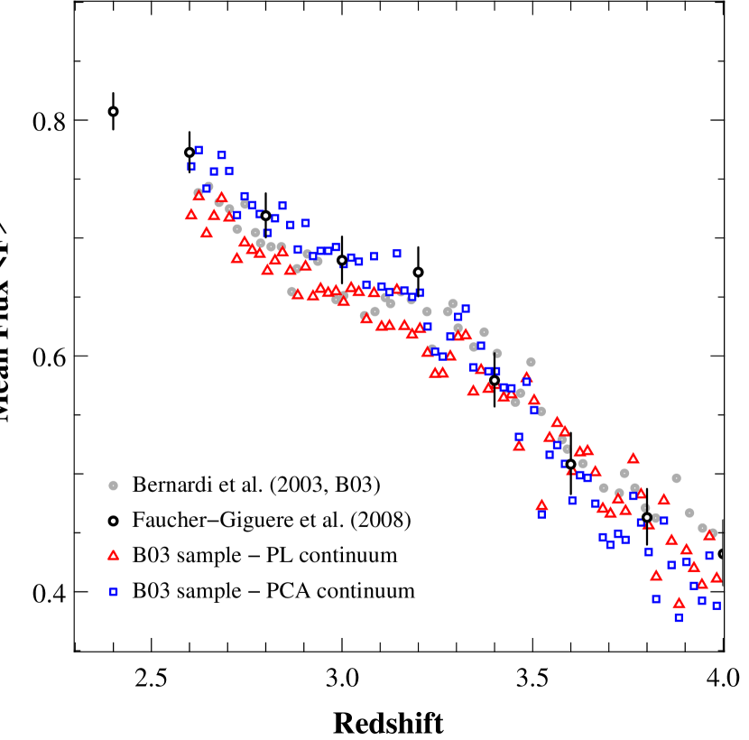
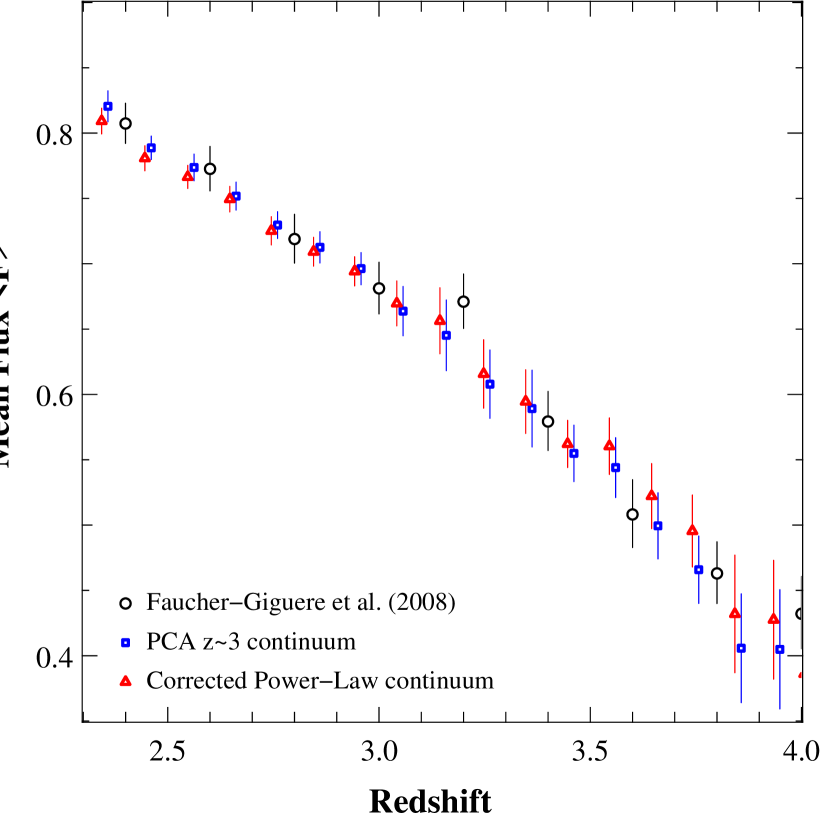
We summarize in Fig. 18 the mean flux evolution measured from the SDSS-DR7 data for a continuum estimated with a PCA (blue squares) or a power law (red triangles) corrected for the systematic bias as seen in Fig. 17. Indeed, the power-law continuum systematically overestimates the amount of absorption in the Lyman-$\alpha$ forest. The mean flux evolution derived with a power-law continuum is corrected by the expected difference seen in mocks between the measured mean flux and the input of the simulation.

There is an excellent agreement between the results of the two methods. Overplotted as black circles on Fig. 18 are the results by Faucher-Giguère et al. (2008) in very good agreement with the PCA estimate except, may be, in the bin around $z\sim 3.2$. Note that the discrepancy is less than 2$\sigma$. In any case, it is apparent that the smooth redshift evolution of the mean flux becomes steeper around redshift $z\sim 3$.

The slight difference between high and intermediate resolution data at $z\sim 3.2$ may be explained by a different selection of the quasars. Indeed, Worseck & Prochaska (2011) have argued that SDSS preferentially selects 3$<$$z_{\rm em}$$<$3.5 quasars with intervening H i Lyman limit systems. However, this should have little influence on the mean flux in the overwhole forest and cannot explain the discrepancy by itself. This could also be due to the possibility that our procedure smoothes out a sharp feature. However, this would be surprising given the width of the bins and the results of our simulations (see Fig. 17).

Figure 18: Mean flux redshift evolution inferred from SDSS-DR7 quasars (red triangles: corrected power-law continuum, and blue squares: $z\sim 3$ PCA continuum) compared to the evolution from Faucher-Giguère et al. (2008) (black open circles). The mean flux evolution derived with a power-law continuum is corrected from the bias predicted in simulation (see Fig. 17). All the measurements are in agreement with each other within errors. No ”bump” is seen in any of the evolution inferred from SDSS-DR7 but there is a definite change in the slope of the evolution at $z\sim 3$ in the sense of a steeper evolution beyond this redshift.

5 Conclusion

The first goal of this paper is to provide a new PCA decomposition of the continuum of $z\sim 3$ quasars. This should be useful for studies of the Lyman-$\alpha$ forest and to generate mock quasar continua to be implemented in simulations constructed to search for systematic effects in future analysis or surveys. We took the opportunity to enlarge to $1020-2000$ Å  the wavelength range over which the spectra are decomposed, to be compared with the previous wavelength range $1020-1600$ Å  used by S05. The mean spectrum at $z\sim 3$ has a similar shape as the mean spectrum derived at $z\sim 1$ by S05 except that the strength of the Lyman-$\alpha$ and C iv emission lines relative to the continuum is smaller at high redshift. Our work concentrates on the estimate of the continuum in the Lyman-$\alpha$ forest and we provide all outputs of this analysis that are required to generate mock continua.

We use this decomposition to revisit the evolution with redshift of the mean flux in the Lyman-$\alpha$ forest and to compare two methods to estimate the quasar flux in the Lyman-$\alpha$ forest: the extrapolation of a power-law fitted to the red part of the spectrum and an estimate of the flux from PCA coefficients.
We find that:
(i) the power law method systematically underestimates the mean flux by an amount decreasing with redshift. When correcting for this bias, as estimated with simulations, we find that the method gives similar results as the PCA method;
(ii) the PCA method yields results very similar to what is measured by Bernardi et al. (2003) and from high spectral resolution data (Faucher-Giguère et al., 2008);
(iii) from our simulations a bump at $z\sim 3.2$, if present, should be marginally detected with the data set of SDSS-DR7;
(iv) finally, from our analysis, we find that there is a definite break in the evolution of the mean flux at $z\sim 3$ in the sense of a steeper decrease of the mean flux at high redshift. We caution that this could be a consequence of a more prominent bump to be slightly smoothed out by our procedures.

The increase of the statistics but most importantly of the quality of the data that will be soon provided by the BOSS survey should definitely settle this issue.