Lightcone renormalization and quantum quenches in one-dimensional Hubbard models

Abstract

The Lieb-Robinson bound implies that the unitary time evolution of an operator can be restricted to an effective light cone for any Hamiltonian with short-range interactions. Here we present a very efficient renormalization group algorithm based on this light cone structure to study the time evolution of prepared initial states in the thermodynamic limit in one-dimensional quantum systems. The algorithm does not require translational invariance and allows for an easy implementation of local conservation laws. We use the algorithm to investigate the relaxation dynamics of double occupancies in fermionic Hubbard models as well as a possible thermalization. For the integrable Hubbard model we find a pure power-law decay of the number of doubly occupied sites towards the value in the long-time limit while the decay becomes exponential when adding a nearest neighbor interaction. In accordance with the eigenstate thermalization hypothesis, the long-time limit is reasonably well described by a thermal average. We point out though that such a description naturally requires the use of negative temperatures. Finally, we study a doublon impurity in a Néel background and find that the excess charge and spin spread at different velocities, providing an example of spin-charge separation in a highly excited state.

1 Introduction

Using ultracold atomic gases as quantum simulators, it has become possible to prepare states in almost perfectly isolated many-body systems and to monitor their time evolution [1, 2, 3, 4, 5, 6]. At the same time, enormous progress in numerical renormalization group methods has given us access to the dynamics of quantum models in one dimension (1D) [7, 8, 9, 10, 11, 12, 13]. These algorithms are all based on approximating a quantum state as a matrix product in an optimally chosen truncated Hilbert space, an idea dating back to the density matrix renormalization group (DMRG) by White [14]. This makes it now possible to study, both experimentally and numerically, fundamental questions about the relaxation dynamics and the role of conservation laws [1, 15]. Furthermore, the applicability of the eigenstate thermalization hypothesis (ETH)—according to which each generic state of a closed quantum system already contains a thermal state which is revealed during unitary time evolution by dephasing [16, 17, 18]—can be investigated as well.

Figure 1: LCRG algorithm. The Trotter-Suzuki decomposition of time evolution reveals the light cone structure.

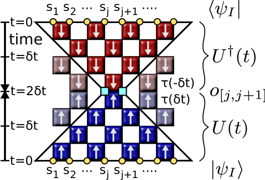
In Sec. 2 we present a new algorithm to study the unitary time evolution of an initial state in a 1D quantum system. We concentrate on the case of a product initial state particularly relevant for experiment but note that the algorithm has been implemented also for thermal initial states. The main idea is to make use of the Lieb-Robinson bound [19] to efficiently simulate the system and to obtain results directly in the thermodynamic limit. Let us briefly recapitulate one of the main results of Refs. [19, 20] which is the basis for our algorithm. We are interested in the time evolution of quantum systems starting from some initial state $|\Psi_{I}\rangle$ where all connected correlation functions decay exponentially with a finite correlation length $\xi$. The time evolution of a local operator $o_{[j,j+n]}$ acting on sites $j,j+1,\ldots,j+n$ can then be approximated by an operator acting only in the effective light cone of the region $[j,j+n]$ (see Fig. 1) while being the identity operator outside of the light cone. More precisely, if $o^{l}_{[j,j+n]}(t)$ is the time evolved operator active only on sites which are at most distance $l$ apart from the region $[j,j+n]$ then

$$||o_{[j,j+n]}(t)-o^{l}_{[j,j+n]}(t)||\leq\text{const}\times\exp\left(-\frac{l-v_{LR}|t|}{\xi}\right)$$ (1)

where $v_{LR}$ is the Lieb-Robinson velocity which is typically, in natural units, of the order of the interaction parameters of the model under consideration [20]. If $v_{LR}|t|\ll l$ then the error of approximating $o_{[j,j+n]}(t)$ by $o^{l}_{[j,j+n]}(t)$ is exponentially small. We show in Sec. 2 that a Trotter-Suzuki decomposition of unitary time evolution immediately leads to a light cone and that this light cone can be represented in a truncated Hilbert space using density matrix renormalization group (DMRG) techniques [14, 21, 22, 23, 24, 25, 26, 9, 27, 28]. In contrast to ground state and transfer matrix DMRG algorithms an explicit calculation of eigenvectors of the system, which is the computationally most costly step, is not necessary. This makes the new light cone renormalization group (LCRG) algorithm extremely fast and efficient. Furthermore, the implementation of local conservation laws—important for an effective numerical study—becomes particularly simple. The “speed of light” set by the Trotter-Suzuki decomposition is typically chosen to be much larger than the Lieb-Robinson speed $v_{LR}$ at which information spreads so that the algorithm directly yields results for the thermodynamic limit. Contrary to the infinite size time evolving block decimation (iTEBD) [13], however, it does not rely on translational invariance. In our paper we will demonstrate these advantages of the LCRG algorithm by studying several examples. At the same time we note that our approach does not solve the most fundamental problem of using matrix product states to investigate the time evolution of one dimensional quantum systems: the linear growth of entanglement entropy with time, which restricts the applicability of such methods to the intermediate time dynamics. It can be shown under very general conditions that this is a fundamental property of unitary time evolution [19, 20] which cannot easily be overcome.

In Sec. 3 we will apply the LCRG algorithm to study the relaxation of a doublon lattice in 1D fermionic Hubbard models. While the problem of a single doublon-holon pair has already been studied in 1D [29], our study is mainly motivated by the experimental and theoretical investigation of the decay of a macroscopic number of doublons in an ultracold fermionic gas on a three-dimensional optical lattice [5, 30]. First, we will present a test of the algorithm by studying the free fermion case where the time evolution can be calculated analytically. Next, we will investigate the differences in the relaxation dynamics between the interacting integrable and non-integrable cases as well as a possible thermalization in the long-time limit. In Sec. 4 we will then demonstrate one of the major advantages of the LCRG algorithm: Even for systems without translational invariance, results in the thermodynamic limit can be obtained. In Sec. 5 we give a brief summary and an outlook on possible future applications of the algorithm. The supplementary material contains the executable code of the LCRG for the anisotropic Heisenberg model, which we have chosen as a simple example, as well as videos of the time evolution for the problem studied in Sec. 4.

2 The light cone renormalization group algorithm

We present the LCRG algorithm to compute the time evolution

$$\langle o_{[j,j+n]}\rangle^{I}(t)\equiv\langle\Psi_{I}|\rme^{\rmi Ht}\,o_{[j,j+n]}\,\rme^{-\rmi Ht}|\Psi_{I}\rangle$$ (2)

of a local operator $o_{[j,j+n]}$ acting on sites $j,j+1,\ldots,j+n$. For the initial state $|\Psi_{I}\rangle=|s_{1}\,s_{2}\,\ldots\rangle$ we consider a product state with $s_{j}$ denoting states in the local basis of dimension $M$. We note that with the help of ancilla sites also thermal states can be expressed using a product initial state followed by an imaginary time evolution, which is also performed using the light-cone algorithm. In this way we have implemented the real time evolution starting, e.g., from a highly entangled quantum state such as the ground state. We consider a Hamiltonian $H=\sum_{j}h_{j,j+1}$ with nearest neighbor interaction; a Trotter-Suzuki decomposition of the unitary time evolution operator then leads to the 2D lattice shown graphically in Fig. 1. It consists of local updates of two neighboring sites forward in time $\tau_{j,j+1}(\delta t)=\exp(-ih_{j,j+1}\delta t)$ (“$\uparrow$” plaquettes) and backward in time $\tau_{j,j+1}(-\delta t)\equiv\tau^{\dagger}_{j,j+1}(\delta t)$ (“$\downarrow$” plaquettes), where $\delta t$ is the Trotter-Suzuki time step. Unless there is an operator insertion, facing plaquettes trivialize and become the identity operator, $\tau_{j,j+1}(-\delta t)\,\tau_{j,j+1}(\delta t)=\mathds{1}$ (shaded plaquettes). This yields the light cone structure emanating from the local observable $o_{[j,j+n]}$ at time $t$. As long as the “speed of light” of the Trotter-Suzuki decomposition is larger than the Lieb-Robinson velocity $v_{LR}$ the expectation value (2) is effectively evaluated in the thermodynamic limit. Neither translational invariance of the initial state nor of the Hamiltonian are required for this construction.

Figure 2: LCRG algorithm. The light cone $C$ grows with each time step by adding first a diagonal left transfer matrix $L$ and then a diagonal right transfer matrix $R$.

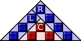
The LCRG algorithm is based on corner transfer matrices [31, 32] to compute the growth of the light cone with each successive time step $\delta t$ (Fig. 2): the light cone $C_{t}$ at time $t$ is multiplied from the left with the diagonal left transfer matrix $L$ and then from the right with the diagonal right transfer matrix $R$ to construct the new light cone for the next time step, $C_{t+\delta t}$. Of course a direct implementation of this procedure would quickly break down because the Hilbert space of light cone states grows exponentially with time. Therefore, we use ideas from DMRG studies of dynamics in stochastic systems [25, 26] to represent both the light cone $C$ and the transfer matrices $L$, $R$ in a reduced Hilbert space of manageable dimension. A fully working implementation of this algorithm specialized to homogeneous systems in included in the supplementary material.

Figure 3: LCRG algorithm. (a)-(c) The light cone $C$ grows to the left by contraction with a left transfer matrix $L$; the left and right transfer matrices $L$ and $R$ are augmented by a local plaquette $\tau(\delta t)$. (d) The reduced density matrix $\rho_{L}$ is constructed from the forward and backward light cones by tracing only over the right site and block indices. (e) The local density matrix is obtained by tracing the forward and backward light cones over both left and right block indices.

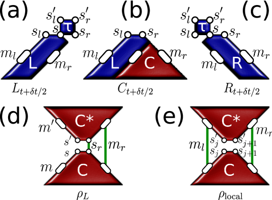
In practice the time evolution proceeds in two half time steps (see Fig. 2). In the first step, the light cone $C_{t}[m_{l}m_{r}]$ has left and right block indices (Fig. 3b) representing states in the (reduced) Hilbert space of dimension $\chi$, while the left transfer matrix $L_{t}[m_{l}s_{l}m_{r}s_{r}]$ has again two block indices but also left and right site indices $s_{l}$, $s_{r}$ of dimension $M$ (Fig. 3a). $L_{t}$ and $C_{t}$ are contracted over their common block index to yield the new light cone $C_{t+\delta t/2}$ half a time step ahead (Fig. 3b):

$$C_{t+\delta t/2}[m_{l}s_{l}s_{r}m_{r}]=\sum_{m}L_{t}[m_{l}s_{l}ms_{r}]\,C_{t}[mm_{r}]\,.$$ (3)

The left transfer matrix $L_{t}$ is enlarged by adding a plaquette at its upper right site index $s_{r}$ (Fig. 3a):

$$L_{t+\delta t/2}[m_{l}s_{l}s_{l}^{\prime}m_{r}s_{r}s_{r}^{\prime}]=\sum_{s}L_{t}[m_{l}s_{l}m_{r}s]\,\tau[s_{l}^{\prime}s_{r}^{\prime}ss_{r}]\,.$$ (4)

Similarly, a local plaquette is attached to the upper left corner of the right transfer matrix $R_{t}$ to construct $R_{t+\delta t/2}$ (Fig. 3c). The initial conditions at $t=0$ are as follows: the block indices represent a single site with dimension $m_{l}=m_{r}=M$, the intial light cone is $C_{t=0}[m_{l}m_{r}]=\Psi_{I}[m_{l}m_{r}]$ for the product initial state $|\Psi_{I}\rangle$ on two neighboring sites, and the transfer matrices have the initial forms $L_{t=0}[m_{l}s_{l}m_{r}s_{r}]=\sum_{s}\Psi_{I}[m_{l}s]\,\tau[s_{l}s_{r}sm_{r}]$ and $R_{t=0}[s_{l}m_{l}s_{r}m_{r}]=\sum_{s}\tau[s_{l}s_{r}m_{l}s]\,\Psi_{I}[sm_{r}]$.

In order to bring $C$, $L$ and $R$ back into their original form the old block index $m$ (dimension $\chi$) is combined with the adjacent site index $s$ (dimension $M$) into a new block index $m^{\prime}=(ms)$ of dimension $\chi^{\prime}=M\chi$. The challenge is to limit the exponential growth of $\chi$ with every time step. This is done by a renormalization step where a reduced density matrix is used to select the $\chi$ most important basis states within the $\chi^{\prime}$-dimensional Hilbert space. The reduced density matrix $\rho_{L}$ for the left block index is formed by combining the forward and backward light cones and tracing over the right site and block indices (Fig. 3d)

$$\rho_{L}[(m^{\prime}s^{\prime})(ms)]=\sum_{s_{r}m_{r}}C_{t+\delta t/2}^{*}[(m^{\prime}s^{\prime})s_{r}m_{r}]\,C_{t+\delta t/2}[(ms)s_{r}m_{r}]$$ (5)

where we have used the fact that in unitary time evolution the backward light cone is the adjoint of the forward light cone. The reduced density matrix $\rho_{L}$ of dimension $\chi^{\prime}$ is by construction hermitean and has unit trace. $\rho_{L}$ is diagonalized, and the $\chi$ states with the largest eigenvalues form the basis of the reduced Hilbert space. Optionally, one can retain all states such that the cumulative weight of the discarded states remains below a given threshold. We use a combination of both to obtain a reliable error control. Finally, the left block index of the light cone $C$ and both block indices of the left transfer matrix $L$ are projected onto this reduced basis, $(m_{l}s_{l})\mapsto m_{l}$. Analogously, the reduced density matrix $\rho_{R}$ is formed by tracing over the left block indices to find a reduced basis for the right block indices, and subsequently the right block index of $C$ and both block indices of $R$ are projected onto the reduced Hilbert space. This completes the first half time step.

The second half of the algorithm works similarly by joining a right transfer matrix $R$ to the right of the light cone (Fig. 2),

$$C_{t+\delta t}[m_{l}s_{l}s_{r}m_{r}]=\sum_{m}C_{t+\delta t/2}[m_{l}m]\,R_{t+\delta t/2}[s_{l}ms_{r}m_{r}]\,.$$ (6)

At this stage the local density matrix

$$\rho_{\text{local}}(t+\delta t)[s_{j}^{\prime}s_{j+1}^{\prime}s_{j}s_{j+1}]=\sum_{m_{l}m_{r}}C_{t+\delta t}^{*}[m_{l}s_{j}^{\prime}s_{j+1}^{\prime}m_{r}]\,C_{t+\delta t}[m_{l}s_{j}s_{j+1}m_{r}]$$ (7)

is formed by contracting the forward and backward light cones over the left and right block indices, leaving open the site indices in the middle (Fig. 3e). The expectation value of a local operator $o_{[j,j+n]}$ is then obtained as

$$\langle o_{[j,j+1]}\rangle^{I}(t+\delta t)=\Tr_{[j,j+1]}\Bigl{(}\rho_{\text{local}}(t+\delta t)\,o_{[j,j+1]}\Bigr{)}.$$ (8)

By multiplying further transfer matrices onto the left or right one can form also the local density matrix $\rho_{[j,j+n]}$ spanning more than two neighboring sites. For example, the density profile to the left of an impurity site is obtained by starting with $\rho_{L}$ and repeatedly multiplying $L$ from the left onto the lower light cone and $L^{*}$ onto the upper light cone, until the desired distance from the impurity is reached. The remaining second half time step proceeds in complete analogy with the first part, growing $L$ and $R$ by one plaquette and renormalizing in turn the left and right block indices.

Note that only summations and multiplications are required to build the light cone. This saves the most time-consuming step in standard transfer matrix DMRG algorithms, where one has to find the largest eigenvector of the transfer matrix. Only the density matrix $\rho_{L,R}$ has to be diagonalized, which dominates the computation time $\mathcal{O}(M^{3}\chi^{3})$. Our algorithm therefore combines the speed of iTEBD [13] with the flexibility of TEBD [12] to treat non-translationally invariant systems. Due to the local structure of the updates, conservation laws are easily implemented in our algorithm (see below). We note that instead of the first order Trotter-Suzuki decomposition shown in Fig. 1 also higher order decompositions can be easily implemented.

3 Doublon decay in Hubbard models

We use the LCRG algorithm with a second order Trotter-Suzuki decomposition to study dynamics in the 1D fermionic Hubbard model

$$H_{U,V}= -J\sum_{j,\sigma=\uparrow,\downarrow}(c^{\dagger}_{j,\sigma}c_{j+1,\sigma}+h.c.)+U\sum_{j}\left(n_{j\uparrow}-\frac{1}{2}\right)\left(n_{j\downarrow}-\frac{1}{2}\right)$$ (9)

$$+V\sum_{j}(n_{j}-1)(n_{j+1}-1)$$

where $J$ is the hopping amplitude, $n_{j,\sigma}=c^{\dagger}_{j,\sigma}c_{j,\sigma}$ and $n_{j}=n_{j\uparrow}+n_{j\downarrow}$ the occupation numbers, $U$ the onsite, and $V$ the nearest-neighbor potential. As initial states we will consider the state $|\Psi_{D}\rangle$, where doubly occupied and empty sites alternate, and the Néel state, $|\Psi_{N}\rangle$. These state are given explicitly by

$$|\Psi_{D}\rangle=\prod_{j}c^{\dagger}_{2j\uparrow}c^{\dagger}_{2j\downarrow}|0\rangle\,,\qquad \qquad|\Psi_{N}\rangle=\prod_{j}c^{\dagger}_{2j+1\uparrow}c^{\dagger}_{2j\downarrow}|0\rangle$$ (10)

where $|0\rangle$ denotes the vacuum. For these states, we want to investigate the time dependence of double occupancies, $d_{j}=n_{j\uparrow}n_{j\downarrow}$, the staggered magnetization, $m_{j}=(-1)^{j}S^{z}_{j}=(-1)^{j}(n_{j\uparrow}-n_{j\downarrow})/2$, and of the operator $w_{j}=(-1)^{j}n_{j}$, measuring the charge imbalance between even and odd sites. Before discussing the numerical results, we first want to establish a number of relations between these three operators in the case where the nearest neighbor repulsion vanishes, $V=0$. The model with $V\neq 0$ will be studied in Sec. 3.4.

3.1 Duality relations for the integrable model

For $V=0$ the model (9) becomes the integrable Hubbard model. Apart from the special symmetries responsible for the integrability of the model by Bethe ansatz, there are other symmetries in this case which allow us to establish various relations between the states and operators:
(a) There is a unitary duality transformation

$$\mathcal{U}=\prod_{j}\Bigl{(}c_{j\uparrow}+(-1)^{j}c^{\dagger}_{j\uparrow}\Bigr{)}$$ (11)

relating the repulsive ($U>0$) and the attractive ($U<0$) Hubbard models. This transformation leads to $\mathcal{U}^{\dagger}c_{j\uparrow}\mathcal{U}=(-1)^{j}c^{\dagger}_{j\uparrow}$, $\mathcal{U}^{\dagger}c_{j\downarrow}\mathcal{U}=c_{j\downarrow}$ so that the kinetic energy part in Eq. (9) stays invariant while $U\to-U$. For the operators we find

$$d_{j} \to n_{j\downarrow}-d_{j},$$ (12)

$$m_{j} \to (-1)^{j}(1-n_{j})/2,$$ (13)

$$w_{j} \to (-1)^{j}(1+n_{j\downarrow}-n_{j\uparrow}).$$ (14)

For the initial state it follows that $\mathcal{U}^{\dagger}|\Psi_{D}\rangle=|\Psi_{N}\rangle$, $\mathcal{U}^{\dagger}|\Psi_{N}\rangle=|\Psi_{D}\rangle$, assuming an even number of lattice sites $L$. For the expectation values (see also Eq. (2))

$$o_{U}^{I}(t)\equiv\sum_{j=1}^{L}\langle o_{j}\rangle^{I}_{U}(t)/L\,,$$ (15)

the duality transformation implies

$$d_{U}^{D}(t) = 1/2-d_{-U}^{N}(t),$$ (16)

$$m_{U}^{N}(t) = -w_{-U}^{D}(t)/2,$$ (17)

$$m_{U}^{D}(t) = -w_{-U}^{N}(t)/2\equiv 0.$$ (18)

The expectation values in the last equation (18) have to vanish identically because of the particle-hole (spin inversion) symmetry of the initial states, respectively. The second identity (17), furthermore, shows that the decay of the staggered magnetization can be studied in a realization of a fermionic Hubbard in cold atomic gases without the need to address the spin degree of freedom directly in a measurement.
(b) On a bipartite lattice, $A\otimes B$, we can furthermore apply the transformation $c_{j\sigma}\to\pm c_{j\sigma}$ for $j\in A$ ($j\in B$), respectively. This leads to $J\to-J$, $U\to U$ and therefore $H_{-U}\to-H_{U}$. This results in $d_{U}^{D}(t)=1/2-d_{U}^{N}(-t)$ and similarly for the other identities.
(c) Finally, we can use the time reversal invariance of the expectation values. Using all three symmetries we find

$$d_{U}^{D}(t) = d_{-U}^{D}(t)=1/2-d_{U}^{N}(t),$$ (19)

$$m_{U}^{N}(t) = m_{-U}^{N}(t)=-w_{U}^{D}(t)/2.$$ (20)

The relaxation dynamics we will consider here is therefore independent of the sign of $U$ and the same information is obtained by starting either from $|\Psi_{D}\rangle$ or $|\Psi_{N}\rangle$.

3.2 Testing the LCRG algorithm: The free fermion case

To test the LCRG algorithm, we first study the free spinful fermion (SFF) case $U=0$ where the dynamics can be calculated exactly. We find $d_{U=0}^{D}(t)=(1+J^{2}_{0}(4Jt))/4$ and $m_{U=0}^{N}(t)=J_{0}(4Jt)/2$ with $J_{0}$ the Bessel function of the first kind.

Figure 4: (a) $m_{0}^{N}(t)$ for free SFF (circles) and for free SLF (squares)—note that the time scale in [33] is stretched by a factor $2$. (b) $d_{0}^{D}(t)$ for free SFF with $\chi$ as indicated. In both cases $\delta t=0.1$ and lines denote the exact results. (c) Absolute error $\delta d_{0}^{D}(t)$ for free SFF with $\chi=5000$ and $\delta t=0.2,0.1,0.05,0.02$ (in arrow direction). (d) $S_{\rm ent}(t)$ for free SFF with $\delta t=0.1$ and $\chi$ as indicated.

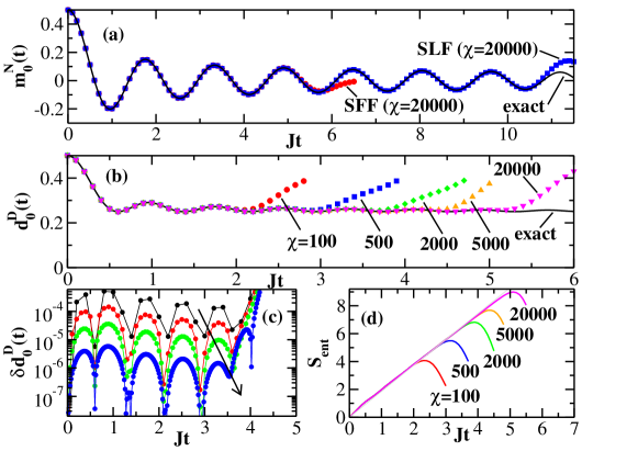
In the free SFF case, the dynamics of electrons with spin up and spin down is completely decoupled. Therefore, we can also use free spinless fermions (SLF) to calculate $m_{0}^{N}(t)$ with a spinless particle representing either the presence of a spin up or a spin down. Then we need to keep only $\sqrt{\chi}$ states to simulate the dynamics with the same accuracy. In Fig. 4(a) the LCRG results for $m_{0}^{N}(t)$ for free SFF and SLF are compared to the exact result. For free SLF with $\chi=20000$ block states we are able resolve $6.5$ oscillations compared to the $5$ oscillations which have been resolved in [33] by iTEBD. We emphasize that for the Hubbard model ($M=4$) with the conservation laws for spin and charge implemented and $\chi=2000$ states kept, each time step takes only $\sim 30$ seconds on a standard PC without parallelization. This is $260\times$ faster and uses $12\times$ less memory than without conservation laws, because the largest diagonal block of the reduced density matrix $\rho_{L,R}$ has only $200$ states. For SLF ($M=2$) the speedup is still $40\times$ with $5\times$ less memory and a largest block of $450$ states. In Fig. 4(b) the results for $d_{0}^{D}(t)$ are shown where $\chi$ is varied. The error of the simulation up to $t_{\rm max}$ where the simulation starts to deviate from the exact result is completely dominated by the error of the Trotter-Suzuki decomposition (see Fig. 4(c)) and is of order $(\delta t)^{2}$ for the second order decomposition used here. Importantly, $t_{\rm max}$ is determined only by $\chi$ and results with in principle arbitrary accuracy can be obtained for $t\in[0,t_{\rm max}]$ by reducing the time step $\delta t$ or using a higher order Trotter-Suzuki decomposition, since the number of RG steps is not restricted.

The algorithm breaks down when the spectrum of the reduced density matrix $\rho_{s}=\rho_{L,R}$ becomes dense. A suitable measure is the entanglement entropy

$$S_{\rm ent}(t)=-\mbox{Tr}\,\rho_{s}\ln\rho_{s}\leq\ln(M\chi)$$ (21)

with $M\chi=\mbox{dim}\,\rho_{s}$. The entanglement entropy is shown in Fig. 4(d) and increases linearly with time. We want to remind the reader once more that the linear increase of the entanglement entropy seems to be a fundamental property of unitary time evolution [20] which cannot easily be overcome and limits the simulation time.

The LCRG algorithm actually does provide an intuitive picture for this behavior: Facing plaquettes outside of the light cone (shown shaded in Fig. 1) trivialize, thereby connecting a local degree of freedom at the edge of the lower light cone with one on the upper light cone by a Kronecker delta. The number of these Kronecker delta bonds between the lower and upper light cone increases linearly with time and determines the entanglement entropy between the light cones. This is very similar to the entanglement entropy of a spin-$1/2$ Heisenberg chain: In this case the ground state can be represented in a resonating valence bond (RVB) basis. If the chain is now split into two semi-infinite segments then the entanglement entropy has been shown to be proportional to the number of RVB bonds connecting the segments [34]. A breakdown of the simulation is observable as a deviation from the linear growth of $S_{\text{ent}}$ and occurs when the entanglement entropy is close to the bound, $S_{\rm ent}(t)\sim\ln(M\chi)$, i.e., when all eigenvalues of $\rho_{s}$ have comparable magnitude thus making further RG steps impossible.

3.3 Results for the Hubbard model

Next, we study $d^{D}_{U}(t)$ in the interacting Hubbard model, a situation which can be realized in ultracold gases [5]. For times $Jt\ll\min\{J/|U|,1\}$ the relaxation is independent of the interaction strength and follows the short-time expansion of the free fermion result $d_{0}^{D}(t)\sim 1/2-2(Jt)^{2}$, see Fig. 5(a). Thus, in order to see the effect of interactions, systems at times $Jt\gg 1/|U|$ have to be studied.

Figure 5: Evolution of double occupancy in Hubbard model. (a) $d^{D}_{U}(t)$ with $\chi=20000$, $\delta t=0.1$ (symbols), and fits (lines), see text. (b) Slope of the entanglement entropy, $S_{\rm ent}\sim aJt$. (c) Fitted exponent $\alpha$ of the power-law decay, see Eq. (22).

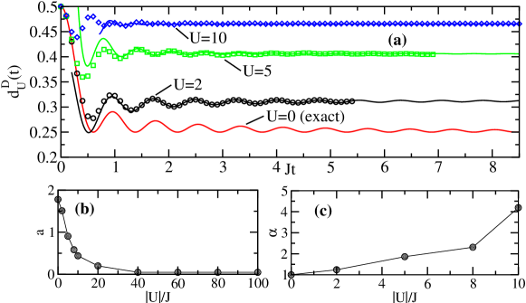
In units of the hopping amplitude $J$ we can simulate longer times the larger $U$ is. This is a consequence of the slower increase of $S_{\rm ent}(t)\sim aJt$ as shown in Fig. 5(b). For large $U$ we find that the slope of the entanglement entropy is given by $a\sim J/|U|$, i.e., the simulation time is proportional to $t_{\rm max}\sim|U|/J^{2}$ and therefore set by the inverse of the magnetic superexchange interaction $\sim J^{2}/|U|$. It is clear that the slope of the entanglement growth becomes smaller the closer the initial state is to an eigenstate of the Hamiltonian: the eigenstate stays invariant under time evolution and no additional entanglement entropy is generated. Comparatively long times can therefore be simulated, in particular, if the time evolution of the ground state with a weak perturbation is studied as, for example, in Ref. [29].

At times $Jt\gg 1$ the relaxation in the free SFF case is given by $d^{D}_{0}(t)=(1+J^{2}_{0}(4Jt))/4\sim[1+(4\pi t)^{-1}(1+\cos(8Jt-\pi/2))]/4$. This motivates us to fit the time dependence at finite $U$ by the function

$$d^{D}_{U}(t)=d_{U}^{D}(\infty)+e^{-\gamma t}[\mathcal{A}+\mathcal{B}\cos(\Omega t-\phi)]/t^{\alpha}$$ (22)

in the regime $1.5<Jt\leq Jt_{\rm max}$. Such fits are shown as solid lines in Fig. 5(a). In all cases $\gamma<10^{-3}$, i.e., we do not find evidence for a finite relaxation rate $\gamma$ . A relaxation following a power law has also been observed at intermediate times in a 1D Bose-Hubbard model starting from an initial state with one boson on every second site [35]. On the other hand, the relaxation for the $XXZ$ model when starting from a Néel state has been interpreted in terms of an exponential decay [33]. Our fits point to a pure power-law decay with an exponent $\alpha$ which increases with increasing $|U|$, see Fig. 5(c). The asymptotic value $d^{D}_{U}(\infty)$ also increases and reaches $1/2$ in the limit $|U|\to\infty$, see the $V=0$ data in Fig. 7(b) below. We emphasize that $d^{D}_{U}(t)=d^{D}_{-U}(t)$, i.e., repulsive interactions lead to a binding of doublons the same way as attractive interactions do [36]. For doublons moving on a 3D lattice it has been argued that for repulsive interactions, $U>0$, much larger than the bandwidth, many-body scattering processes are needed to dissipate the doublon energy, which leads to an exponentially small relaxation rate $\gamma\sim\exp(-U/J)$ [30, 5]. In our simulations we do not see indications for a corresponding crossover time scale $\sim 1/\gamma$ at which exponential relaxation might set in. The power law decay in the Hubbard model (or, at least, the very small relaxation rate) might be a consequence of the infinitely many local conservation laws leading to integrability. It is important to stress, however, that our numerical data for the intermediate time dynamics cannot finally resolve the question whether or not exponential relaxation does exist. In the next paragraph we will, however, give further support that the fits with Eq. (22) describe the relaxation at long times correctly by showing that the the asymptotic value $d_{U}^{D}(\infty)$ obtained from the fits agrees very well with a thermal expectation value.

3.3.1 Long-time limit and thermalization

According to the eigenstate thermalization hypothesis (ETH) [16, 17], each initial state—which can be represented as a superposition of eigenstates of the Hamiltonian—already contains a thermal state. This thermal state is revealed during time evolution due to dephasing effects between the different eigenstates. We say that the system has thermalized if the long-time average

$$\bar{o}=\lim_{\tau\to\infty}\frac{1}{\tau}\int_{0}^{\tau}dt\langle\Psi_{I}|o(t)|\Psi_{I}\rangle$$ (23)

is equal to the thermal average $\langle o\rangle_{\rm\lambda_{i}}$ in an appropriately chosen ensemble with the intensive variables $\lambda_{i}$. Note that this definition only demands that $\bar{o}=\langle o\rangle_{\rm\lambda_{i}}$, i.e., time dependent fluctuations in $\langle\Psi_{I}|o(t)|\Psi_{I}\rangle$ can, in principle, remain large even for $t\to\infty$. This will, in particular, be true for free models where no relaxation mechanisms exist and the concept of thermalization therefore has limited meaning. In interacting models, on the other hand, we expect that $o(t\to\infty)\equiv\bar{o}$, i.e., time-dependent fluctuations vanish in the long-time limit. In this case, the system is expected to have truly thermalized if $o(t\to\infty)=\langle o\rangle_{\rm\lambda_{i}}$.

The appropriate thermal ensemble is determined by the set of conserved quantities $Q_{i}$ with $[H,Q_{i}]=0$. Obviously, $\langle\Psi_{I}|Q_{i}(t)|\Psi_{I}\rangle=\mbox{const}$ which means that the intensive variables (Lagrange multipliers) $\lambda_{i}$ have to be determined such that

$$\langle\Psi_{I}|Q_{i}|\Psi_{I}\rangle\equiv\langle Q_{i}\rangle_{\rm\lambda_{i}}.$$ (24)

Every quantum system has two types of conserved quantities: local and non-local. We call a conserved quantity local if it can be expressed as a sum of local densities acting only on a finite number of lattice sites. For a generic system, usually only very few local conserved quantities such as the particle number operator and the Hamiltonian itself exist. Any quantum system in the thermodynamic limit has, on the other hand, infinitely many non-local conserved quantities, as, for example, the projection operators $|E_{n}\rangle\langle E_{n}|$ onto the eigenstates of the system. It is not clear if these non-local conserved quantities play any role in determining thermalization or transport [37, 10, 11]. In studies of thermalization they are usually simply neglected.

The 1D Hubbard model is integrable by Bethe ansatz and has infinitely many local conserved quantities which can be constructed explicitly from a family of commuting transfer matrices [38, 39]. In this case, one should, in principle, consider a generalized Gibbs ensemble with a Lagrange multiplier $\lambda_{i}$ for each local conservation law. However, such ensembles are impossible to handle in the thermodynamic limit except for the simplest free particle models [18]. Here we will instead consider the usual canonical ensemble. The effective temperature $T_{\rm eff}$ then acts as a Lagrange multiplier determined such that

$$\langle\Psi_{D}|H|\Psi_{D}\rangle/L=\frac{1}{LZ}\Tr\left\{H\rme^{-H/T_{\rm eff}}\right\}$$ (25)

where $Z=\Tr\rme^{-H/T_{\rm eff}}$ is the partition function and the energy $\langle\Psi_{D}|H|\Psi_{D}\rangle/L=U/4$ is conserved during time evolution. Since the spectrum of eigenenergies per site is bounded for a lattice model, the use of negative temperatures is natural with $1/T\to 0^{\pm}$ corresponding to the case of maximum entropy. In the following we denote the thermal average in the canonical ensemble by $\langle d\rangle_{U,T}$ and it is easy to see that $\langle d\rangle_{U,T}=\langle d\rangle_{-U,-T}$ holds. The duality transformation (11), (16) furthermore implies $\langle d\rangle_{U,T}+\langle d\rangle_{-U,T}=1/2$ for all $T$. In particular, $\langle d\rangle_{U>0,T>0}<1/4$ and $\langle d\rangle_{U<0,T>0}>1/4$ with both being equal to $1/4$ in the limit $T\to\infty$. We calculate the thermal average $\langle d\rangle_{U,T}$ using a transfer-matrix DMRG algorithm [21, 22, 40, 41] and find that $T_{\rm eff}$ is negative (positive) for the repulsive (attractive) model, respectively. The dependence of the effective temperature $T_{\rm eff}$ on interaction strength is shown in Fig. 7(a) together with the results for the extended Hubbard model which are discussed in the next subsection. The comparison between the double occupancy extrapolated in time, $d^{D}_{U}(\infty)$, and the thermal double occupancy $\langle d\rangle_{T_{\rm eff}}$ shown in Fig. 7(b) yields excellent agreement. This seems to suggest, on the one hand, that the extrapolation using Eq. (22) is appropriate leaving very little room for an additional exponential decay which possibly could set in at a longer time scale. On the other hand, it also seems to suggest that the other local conservation laws of the Hubbard model have very little influence on the relaxation of double occupancies. To qualitatively understand the latter property we can think of writing the operator $d$ as a sum of projections onto all the conserved quantities which form a basis of the operator space [37, 10]. At least for large $U$ it is then clear that the projection onto the Hamiltonian, which does contain the operator $d$ itself, will give the dominant contribution to the thermal expectation value.

3.4 Results for the extended Hubbard model

Finally, we consider the non-integrable extended Hubbard model obtained by turning on the next-nearest neighbor repulsion $V$ in Eq. (9). The duality relations used for the Hubbard model are then no longer valid because $V\sum_{j}(n_{j}-1)(n_{j+1}-1)\to 4V\sum_{j}S^{z}_{j}S^{z}_{j+1}$ under the duality tranformation, Eq. (11). However, we still have $d^{D}_{U,V}(t)=d^{D}_{-U,-V}(t)$ for the time evolution and $\langle d\rangle_{U,V,T}=\langle d\rangle_{-U,-V,-T}$ for the thermal expectation value since these relations only rely on the lattice being bipartite and time reversal symmetry. We focus in the following on $V\leq U/2$ corresponding to a spin-density wave state in the ground state phase diagram [40, 41]. We note that for $V>U/2$, $|\Psi_{D}\rangle$ is close to the charge-density wave (CDW) ground state and long simulations in time are possible with $d^{D}_{U,V}(t)$ staying close to $1/2$ and showing revival oscillations (data not shown). For the case $V=U/2$—which is approximately at the phase transition line from the spin-density to a charge-density wave state [40, 41]—we find a qualitatively different behavior than in the Hubbard model (see Fig. 6).

Figure 6: Extended Hubbard model: $d^{D}_{U,V}(t)$ for $V=U/2$ with $\chi=10000$, $\delta t=0.1$ (symbols), and fits (lines). Inset: Relaxation rate $\gamma$ extracted from the fits.

Here $d_{U,V}^{D}(t)$ decreases at long times with increasing interaction strength. In general, $d_{U,V}^{D}(t)$ can increase or decrease at long times with increasing interaction strength depending on the ratio $V/U$. Using the same fit function (22) as before we find that it is no longer possible to describe the relaxation dynamics by a pure power law decay. Instead, we now find a finite relaxation rate $\gamma$ as shown in the inset of Fig. 6.

3.4.1 Long-time limit and thermalization

Investigating again a possible thermalization we can shed some light on the observed dependence of the extrapolated value $d_{U,V}^{D}(\infty)$ on the ratio $V/U$. For $V\neq 0$ the model is no longer integrable and—if thermalization does occur—the final state should be fully described by the canonical ensemble. The energy during the time evolution is now fixed to

$$\langle\Psi_{D}|H|\Psi_{D}\rangle/L=\frac{U}{4}-V$$ (26)

and determines via the relation (25) the effective temperature shown in Fig. 7(a). For $V=U/4$ it follows that $1/T_{\rm eff}=0$ and $\langle d\rangle_{U,V=U/4}=1/4$. In the repulsive case, $U>0$, the energy (26) is negative for $V>U/4$ leading to $T_{\rm eff}>0$. For $V<U/4$, on the other hand, the energy is positive and therefore $T_{\rm eff}<0$. For $U<0$ the signs of $T_{\rm eff}$ are reversed.

Figure 7: (a) Inverse effective temperatures for different ratios of $V/U$ with $U>0$. $T_{\rm eff}$ changes sign for $U<0$. (b) $d^{D}_{U,V}(\infty)$ (filled symbols connected by solid lines) compared to the thermal average $\langle d\rangle_{\rm T_{eff}}$ (open symbols connected by dashed lines).

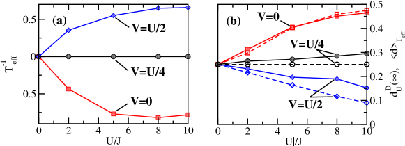
Using again a transfer matrix DMRG algorithm to calculate the thermal expectation value $\langle d\rangle_{\rm T_{eff}}$ at temperatures $T_{\rm eff}$ we can compare with the extrapolated value $d^{D}_{U,V}(\infty)$ from the time evolution, see Fig. 7(b). Compared to the pure Hubbard model the agreement is not quite as good and the deviations increase the closer the ratio of the interactions is to the critical line $V=U/2$ and also the larger $U$ is. This does suggest—assuming that the system will finally thermalize—that the numerically obtained intermediate time dynamics is not sufficient to fully extract the long time behavior. A possible explanation is that two different relaxation processes exist in this case: a fast one at short time scales leading to a pre-thermalized state and a slower one setting in at $Jt\gg\exp(U/J)$ [30, 5]. This might also explain the non-monotonic behavior of $\gamma(U,V/U=\mbox{const})$ obtained when fitting with a single relaxation rate, see inset of Fig. 6.

4 Application to a non-translationally invariant case

On of the main advantages of the LCRG algorithm is that it allows to study the time evolution of one-dimensional quantum systems in the thermodynamic limit even if the initial state and/or the Hamiltonian are not translationally invariant. As an example, we consider the time evolution in the $V=0$ Hubbard model (9) of the non-translationally invariant state

$$|\tilde{\Psi}_{N}\rangle=c^{\dagger}_{0\uparrow}|\Psi_{N}\rangle=c^{\dagger}_{0\uparrow}\prod_{j}c^{\dagger}_{2j+1\uparrow}c^{\dagger}_{2j\downarrow}|0\rangle$$ (27)

obtained by adding an additional electron at site $j=0$ to the Néel state, Eq. (10). In Fig. 8, LCRG results for the dynamics of the excess charge and the excess spin defined by

$$\langle n^{\rm exc}_{j}\rangle=\langle n_{j}\rangle-\langle n_{j}^{\rm bg}\rangle\,;\qquad\langle s^{\rm exc}_{j}\rangle=\langle s_{j}\rangle-\langle s_{j}^{\rm bg}\rangle$$ (28)

are shown for $U/J=2$. Here $\langle n_{j}^{\rm bg}\rangle\equiv 1$ ($\langle s_{j}^{\rm bg}\rangle$) are the background charge (spin) densities, respectively, obtained from the time evolution of $|\Psi_{N}\rangle$, i.e., from a system without the additional electron.

Figure 8: Time evolution starting from the initial state $|\tilde{\Psi}_{N}\rangle$, Eq. (27), for $U/J=2$ with $\chi=1024$ states kept. Shown are results for times $Jt=3,2.4,1.8,\cdots,0$ (from bottom to top) for (a) the excess charge $\langle n^{\rm exc}_{j}\rangle$, and (b) the excess spin $\langle s^{\rm exc}_{j}\rangle$. Subsequent curves are shifted by $0.2$ for clarity of presentation. The dashed lines connect the points $x_{c(s)}$, see Fig. 9.

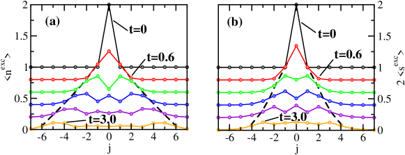
Videos of the time evolution for several other interaction strengths $U/J$ are presented in the supplementary material. We observe that $\langle n^{\rm exc}_{j}\rangle$ and $\langle s^{\rm exc}_{j}\rangle$ spread out into the lattice with different velocities clearly revealing the light-cone structure. For the non-translationally invariant problem considered here we have not implemented the conservation laws yet and the results shown in Fig. 8 have been obtained by keeping a relatively moderate number of states, $\chi=1024$. Although the simulation time is therefore smaller than in the translationally invariant cases discussed in the previous chapters, we want to stress that the evolution of the Néel background is simulated in the thermodynamic limit and thus very different from that in a small system tractable, for example, by exact diagonalization.

Different charge and spin velocities for the one-dimensional Hubbard model starting from an initial non-equilibrium state have already been observed in Ref. [42]. In this case, an initial state was considered where the ground state was perturbed by a small local charge and spin imbalance thus allowing to extract the velocities of the elementary spin and charge excitations which can also be obtained by Bethe ansatz. Our initial state, on the other hand, is a highly excited state and the charge and spin velocities are not related to those of the elementary excitations.

To extract the charge velocity $v_{c}$ and the spin velocity $v_{s}$ for our initial state we take the point $x_{c(s)}(t)$ where the tail has reached half of the height of the first peak of the charge (spin) distribution as reference point.

Figure 9: (a) Time evolution of the reference points $x_{c(s)}$ as defined in the text for the excess charge (circles) and for the excess spin (squares) with $U/J=2$. The lines are linear fits. (b) Charge and spin velocities as a function of $U/J$.

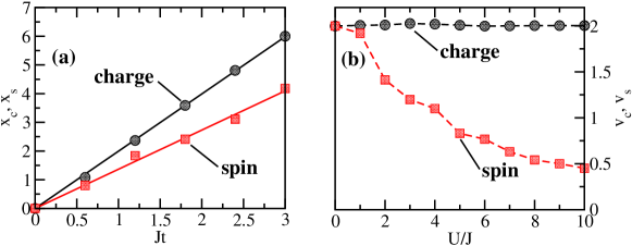
Fig. 9(a) shows that $x_{c(s)}(t)$ depends linearly on time. The dependence of the velocities on the interaction strength $U/J$ is shown in Fig. 9(b). We find a charge velocity $v_{c}\approx 2J$ independent of $U$. For $U=0$ the charge and spin distributions are identical for all times and $v_{s}=v_{c}$, but for increasing $U$ the spin velocity $v_{s}$ decreases. These results can be qualitatively understood as follows: the excess charge sees a uniformly charged background and therefore moves unimpeded with the Fermi velocity $v_{F}$ of the non-interacting system, $v_{c}\approx v_{F}=2J$. The excess magnetization, on the other hand, moves with a velocity proportional to the effective spin superexchange $\sim J^{2}/U$ which therefore decreases with increasing $U$. For large $U$ we find, furthermore, that the spin dynamics becomes more complicated. While most of the excess magnetization remains inert in this limit, an additional small staggered part appears which spreads out with a velocity close to the charge velocity (data not shown).

5 Conclusions

The development of new spectroscopic techniques to study ultracold quantum gases on optical lattices with very good spatial and time resolution has put the topic of non-equilibrium dynamics in quantum systems firmly back onto the agenda. Particularly interesting from a fundamental persepective is the dynamics in one dimension where many of the standard lattice models such as the Heisenberg, the $t-J$, and the Hubbard model are integrable, i.e., these systems have an infinite number of local conservation laws. Since a conserved quantity stays invariant under time evolution, the presence of many conserved quantities is expected to severely restrict the dynamics of the quantum system as a whole and might even prevent the system from reaching thermal equilibrium. To investigate such questions numerically, different algorithms have been developed: The time-dependent density-matrix renormalization group (t-DMRG) and the time-evolving block decimation (TEBD), in particular, allow one to access the intermediate time dynamics by representing the time evolved state as a matrix product state. Among the aims when developing numerical algorithms to study the time evolution are (a) the thermodynamic limit, (b) the flexibility to simulate different systems, (c) a high computational efficiency, and (d) to simulate the system for as long as possible.

Here we have presented a new algorithm which does make progress concerning many of the points mentioned above. The light cone renormalization group (LCRG) algorithm is highly efficient by simulating at each time step only that part of the lattice (a light cone) which is affected by the time evolution. The results obtained are directly for the thermodynamic limit. Contrary to the infinite size TEBD, the LCRG algorithm does not rely on translational invariance. It is therefore extremely flexible and can, in particular, also deal with non-translationally invariant problems. It cannot, however, simulate the quantum system for times significantly longer than other algorithms based on matrix product states. We have shown that the lattice path integral representation of unitary time evolution—forming the basis for the LCRG algorithm—provides a simple picture for the linear entanglement growth with time which restricts the simulation time of such algorithms. An executable sample code for the anisotropic Heisenberg model is provided in the supplementary material.

We used the LCRG algorithm to study quench dynamics in the integrable Hubbard model starting from a state with every second site doubly occupied and found indications for a pure power-law relaxation. For the extended non-integrable Hubbard model, on the contrary, the relaxation appears to be exponential. In both cases we found that the time evolved state in the long-time limit seems to be close to a thermal state supporting the eigenstate thermalization hypothesis.

Finally, we demonstrated that the LCRG algorithm can also be used to study the time evolution of non-translationally invariant initial states. For the Néel state with one site occupied by a doublon we showed that the excess charge and excess spin spread with finite, but different, velocities. We extracted the dependence of the velocities on the strength of the Hubbard interaction $U$ which can be used for comparison with future experiments. Videos of the time evolution for different parameter sets can be found in the supplementary material.

As an outlook we want to emphasize that future applications of the LCRG algorithm to other non-translationally invariant setups such as impurity problems, disorder, and to systems with trapping potentials are feasible.

References

- [1] Kinoshita T, Wenger T and Weiss D S 2006 Nature 440 900
- [2] Hofferberth S, Lesanovsky I, Fischer B, Schumm T and Schmiedmayer J 2007 Nature 449 324
- [3] Gericke T, Würtz P, Reitz D, Langen T and Ott H 2008 Nat. Phys. 4 949
- [4] Würtz P, Langen T, Gericke T, Koglbauer A and Ott H 2009 Phys. Rev. Lett. 103 080404
- [5] Strohmaier N, Greif D, Jördens R, Tarruell L, Moritz H, Esslinger T, Sensarma R, Pekker D, Altman E and Demler E 2010 Phys. Rev. Lett. 104 080401
- [6] Sensarma R, Pekker D, Altman E, Demler E, Strohmaier N, Greif D, Jördens R, Tarruell L, Moritz H and Esslinger T 2010 Phys. Rev. B 82 224302
- [7] Daley A J, Kollath C, Schollwöck U and Vidal G 2004 J. Stat. Mech. P04005
- [8] Feiguin A E and White S R 2005 Phys. Rev. B 72 220401(R)
- [9] Sirker J and Klümper A 2005 Phys. Rev. B 71 241101(R)
- [10] Sirker J, Pereira R G and Affleck I 2009 Phys. Rev. Lett. 103 216602
- [11] Sirker J, Pereira R G and Affleck I 2011 Phys. Rev. B 83 035115
- [12] Vidal G 2003 Phys. Rev. Lett. 91 147902
- [13] Vidal G 2007 Phys. Rev. Lett. 98 070201
- [14] White S R 1992 Phys. Rev. Lett. 69 2863
- [15] Rigol M, Dunjko V and Olshanii M 2008 Nature 452 854–858
- [16] Deutsch J M 1991 Phys. Rev. A 43 2046–2049
- [17] Srednicki M 1994 Phys. Rev. E 50 888–901
- [18] Cassidy A C, Clark C W and Rigol M 2011 Phys. Rev. Lett. 106 140405
- [19] Lieb E H and Robinson D W 1972 Comm. Math. Phys. 28 251–257
- [20] Bravyi S, Hastings M B and Verstraete F 2006 Phys. Rev. Lett. 97 050401
- [21] Bursill R, Gehring G A, Farnell D J J, Parkinson J B, Xiang T and Zeng C 1995 J. Phys: Cond. Mat. 7 8605
- [22] Wang X and Xiang T 1997 Phys. Rev. B 56 5061
- [23] Kemper A, Schadschneider A and Zittartz J 2001 J. Phys. A 34 L279
- [24] Enss T and Schollwöck U 2001 J. Phys. A 34 7769
- [25] Kemper A, Gendiar A, Nishino T, Schadschneider A and Zittartz J 2003 J. Phys. A 36 29
- [26] Enss T, Henkel M, Picone A and Schollwöck U 2004 J. Phys. A: Math. Gen. 37 10479
- [27] Hastings M B 2009 J. Math. Phys. 50 095207
- [28] Bañuls M C, Hastings M B, Verstraete F and Cirac J I 2009 Phys. Rev. Lett. 102 240603
- [29] Al-Hassanieh K A, Reboredo F A, Feiguin A E, González I and Dagotto E 2008 Phys. Rev. Lett. 100 166403
- [30] Rosch A, Rasch D, Binz B and Vojta M 2008 Phys. Rev. Lett. 101 265301
- [31] Baxter R J 1982 Exactly Solved Models in Statistical Mechanics (London: Academic Press)
- [32] Nishino T and Okunishi K 1996 J. Phys. Soc. Jpn. 65 891
- [33] Barmettler P, Punk M, Gritsev V, Demler E and Altman E 2009 Phys. Rev. Lett. 102 130603
- [34] Alet F, Capponi S, Laflorencie N and Mambrini M 2007 Phys. Rev. Lett. 99 117204
- [35] Cramer M, Flesch A, McCulloch I P, Schollwöck U and Eisert J 2008 Phys. Rev. Lett. 101 063001
- [36] Winkler K, Thalhammer G, Lang F, Grimm R, Hecker Denschlag J, Daley A J, Kantian A, Büchler H P and Zoller P 2006 Nature 441 853
- [37] Jung P and Rosch A 2007 Phys. Rev. B 76 245108
- [38] Shastry B 1986 Phys. Rev. Lett. 56 1529
- [39] Zotos X, Naef F and Prelovšek P 1997 Phys. Rev. B 55 11029
- [40] Nakamura M 2000 Phys. Rev. B 61 16377
- [41] Glocke S, Klümper A and Sirker J 2007 Phys. Rev. B 76 155121
- [42] Kollath C, Schollwöck U and Zwerger W 2005 Phys. Rev. Lett. 95 176401