YITP-SB-11-11

SUSY QCD corrections to Higgs-b Production: Is the ΔbsubscriptΔ𝑏\Delta_{b} Approximation Accurate?

S. Dawsona, C. B. Jacksonb, P. Jaiswala,c aDepartment of Physics, Brookhaven National Laboratory, Upton, NY 11973, USA
b Physics Department, University of Texas, Arlington, Texas
cYang Institute for Theoretical Physics, Stony Brook University, Stony Brook, NY 11790, USA
Abstract

The associated production of a Higgs boson with a b𝑏b quark is a discovery channel for the lightest MSSM neutral Higgs boson. We consider the SUSY QCD contributions from squarks and gluinos and discuss the decoupling properties of these effects. A detailed comparison of our exact 𝒪(αs)𝒪subscript𝛼𝑠{\cal O}(\alpha_{s}) results with those of a widely used effective Lagrangian approach, the ΔbsubscriptΔ𝑏\Delta_{b} approximation, is presented. The ΔbsubscriptΔ𝑏\Delta_{b} approximation is shown to accurately reproduce the exact one-loop SQCD result to within a few percent over a wide range of parameter space.

I Introduction

Once a light Higgs-like particle is discovered it will be critical to determine if it is the Higgs Boson predicted by the Standard Model. The minimal supersymmetric Standard Model (MSSM) presents a comparison framework in which to examine the properties of a putative Higgs candidate. The MSSM Higgs sector contains 555 Higgs bosons–222 neutral bosons, hh and H𝐻H, a pseudoscalar boson, A𝐴A, and 222 charged bosons, H±superscript𝐻plus-or-minusH^{\pm}. At the tree level the theory is described by just 222 parameters, which are conveniently chosen to be MAsubscript𝑀𝐴M_{A}, the mass of the pseudoscalar boson, and tanβ𝛽\tan\beta, the ratio of vacuum expectation values of the 222 neutral Higgs bosons. Even when radiative corrections are included, the theory is highly predictiveDjouadi (2005); Gunion et al. (1990); Carena and Haber (2003).

In the MSSM, the production mechanisms for the Higgs bosons can be significantly different from in the Standard Model. For large values of tanβ𝛽\tan\beta, the heavier Higgs bosons, A𝐴A and H𝐻H, are predominantly produced in association with b𝑏b quarks. Even for tanβ5similar-to𝛽5\tan\beta\sim 5, the production rate in association with b𝑏b quarks is similar to that from gluon fusion for A𝐴A and H𝐻H productionDittmaier et al. (2011). For the lighter Higgs boson, hh, for tanβ >7 >𝛽7\tan\beta\mathrel{\hbox to0.0pt{\lower 4.0pt\hbox{\hskip 1.0pt$\sim$}\hss}\raise 1.0pt\hbox{$>$}}7 the dominant production mechanism at both the Tevatron and the LHC is production with b𝑏b quarks for light MAsubscript𝑀𝐴M_{A} ( <200GeV <absent200𝐺𝑒𝑉\mathrel{\hbox to0.0pt{\lower 4.0pt\hbox{\hskip 1.0pt$\sim$}\hss}\raise 1.0pt\hbox{$<$}}200~{}GeV), where the bb¯h𝑏¯𝑏b{\overline{b}}h coupling is enhanced . Both the TevatronBenjamin et al. (2010) and the LHC experimentsChatrchyan et al. (2011) have presented limits Higgs production in association with b𝑏b quarks, searching for the decays hτ+τsuperscript𝜏superscript𝜏h\rightarrow\tau^{+}\tau^{-} and bb¯𝑏¯𝑏b\overline{b}111The expected sensitivities of ATLAS and CMS to b𝑏b Higgs associated production are described in Refs. Aad et al. (2009); Bayatian et al. (2007).. These limits are obtained in the context of the MSSM are sensitive to the b𝑏b-squark and gluino loop corrections which we consider here.

The rates for bh𝑏bh associated production at the LHC and the Tevatron have been extensively studiedDawson et al. (2006); Campbell et al. (2004); Maltoni et al. (2003); Dawson et al. (2005); Dittmaier et al. (2004); Dicus et al. (1999); Dawson et al. (2004); Maltoni et al. (2005); Campbell et al. (2003); Carena et al. (2007, 1999) and the NLO QCD correction are well understood, both in the 444- and 555- flavor number parton schemesDawson et al. (2006); Campbell et al. (2004); Maltoni et al. (2003). In the 444- flavor number scheme, the lowest order processes for producing a Higgs boson and a b𝑏b quark are ggbb¯h𝑔𝑔𝑏¯𝑏gg\rightarrow b{\overline{b}}h and qq¯bb¯h𝑞¯𝑞𝑏¯𝑏q{\overline{q}}\rightarrow b{\overline{b}}hDittmaier et al. (2004); Dawson et al. (2005); Dicus et al. (1999). In the 5limit-from55- flavor number scheme, the lowest order process is bgbh𝑏𝑔𝑏bg\rightarrow bh (b¯gb¯h¯𝑏𝑔¯𝑏{\overline{b}}g\rightarrow{\overline{b}}h). The two schemes represent different orderings of perturbation theory and calculations in the two schemes produce rates which are in qualitative agreementCampbell et al. (2004); Dittmaier et al. (2011). In this paper, we use the 555-flavor number scheme for simplicity. The resummation of threshold logarithmsField et al. (2007), electroweak correctionsDawson and Jaiswal (2010); Beccaria et al. (2010) and SUSY QCD correctionsDawson and Jackson (2008) have also been computed for bh𝑏bh production in the 5limit-from55- flavor number scheme.

Here, we focus on the role of squark and gluino loops. The properties of the SUSY QCD corrections to the bb¯h𝑏¯𝑏b{\overline{b}}h vertex, both for the decay hbb¯𝑏¯𝑏h\rightarrow b{\overline{b}}Dabelstein (1995); Hall et al. (1994); Carena et al. (2000); Guasch et al. (2003) and the production, bb¯h𝑏¯𝑏b{\overline{b}}\rightarrow hHaber et al. (2001); Harlander and Kilgore (2003); Guasch et al. (2003); Dittmaier et al. (2004), were computed long ago. The contributions from b𝑏b squarks and gluinos to the lightest MSSM Higgs boson mass are known at 222-loopsHeinemeyer et al. (2005); Brignole et al. (2002), while the 222-loop SQCD contributions to the bb¯h𝑏¯𝑏b{\overline{b}}h vertex is known in the limit in which the Higgs mass is much smaller than the squark and gluino massesNoth and Spira (2010, 2008). The contributions of squarks and gluinos to the on-shell bb¯h𝑏¯𝑏b{\overline{b}}h vertex are non-decoupling for heavy squark and gluino masses and decoupling is only achieved when the pseudoscalar mass, MAsubscript𝑀𝐴M_{A}, also becomes large.

An effective Lagrangian approach, the ΔbsubscriptΔ𝑏\Delta_{b} approximationCarena et al. (2000); Hall et al. (1994), can be used to approximate the SQCD contributions to the on-shell bb¯h𝑏¯𝑏b{\overline{b}}h vertex and to resum the (αstanβ/MSUSY)nsuperscriptsubscript𝛼𝑠𝛽subscript𝑀𝑆𝑈𝑆𝑌𝑛(\alpha_{s}\tan\beta/M_{SUSY})^{n} enhanced terms. The numerical accuracy of the ΔbsubscriptΔ𝑏\Delta_{b} effective Lagrangian approach has been examined for a number of cases. The 2limit-from22-loop contributions to the lightest MSSM Higgs boson mass of 𝒪(αbαs)𝒪subscript𝛼𝑏subscript𝛼𝑠{\cal O}(\alpha_{b}\alpha_{s}) were computed in Refs. Heinemeyer et al. (2005) and Brignole et al. (2002), and it was found that the majority of these corrections could be absorbed into a 1limit-from11-loop contribution by defining an effective b𝑏b quark mass using the ΔbsubscriptΔ𝑏\Delta_{b} approach. The sub-leading contributions to the Higgs boson mass (those not absorbed into ΔbsubscriptΔ𝑏\Delta_{b}) are then of 𝒪(1GeV)𝒪1𝐺𝑒𝑉{\cal O}(1~{}GeV). The ΔbsubscriptΔ𝑏\Delta_{b} approach also yields an excellent approximation to the SQCD corrections for the decay process hbb¯𝑏¯𝑏h\rightarrow b{\overline{b}}Guasch et al. (2003). It is particularly interesting to study the accuracy of the ΔbsubscriptΔ𝑏\Delta_{b} approximation for production processes where one of the b𝑏b quarks is off-shell. The SQCD contributions from squarks and gluinos to the inclusive Higgs production rate in association with b𝑏b quarks has been studied extensively in the 4FNS in Ref. Dittmaier et al. (2007), where the the lowest order contribution is ggbb¯h𝑔𝑔𝑏¯𝑏gg\rightarrow b{\overline{b}}h. In the 4FNS, the inclusive cross section including the exact 1-loop SQCD corrections is reproduced to within a few percent using the ΔbsubscriptΔ𝑏\Delta_{b} approximation. However, the accuracy of the ΔbsubscriptΔ𝑏\Delta_{b} approximation for the MSSM neutral Higgs boson production in the 5FNS has been studied for only a small set of MSSM parameters in Ref. Dawson and Jackson (2008). The major new result of this paper is a detailed study of the accuracy of the ΔbsubscriptΔ𝑏\Delta_{b} approach in the 5FNS for the bgbh𝑏𝑔𝑏bg\rightarrow bh production process. In this case, one of the b𝑏b quarks is off-shell and there are contributions which are not contained in the effective Lagrangian approach.

The plan of the paper is as follows: Section 222 contains a brief review of the MSSM Higgs and b𝑏b squark sectors and also a review of the effective Lagrangian approximation. The calculation of Ref. Dawson and Jackson (2008) is summarized in Section 2. We include SQCD contributions to bh𝑏bh production which are enhanced by mbtanβsubscript𝑚𝑏𝛽m_{b}\tan\beta which were omitted in Ref. Dawson and Jackson (2008). Analytic results for the SQCD corrections to bgbh𝑏𝑔𝑏bg\rightarrow bh in the extreme mixing scenarios in the b𝑏b squark sector are presented in Section 3. Section 4 contains numerical results for the s=7𝑠7\sqrt{s}=7 TeV LHC. Finally, our conclusions are summarized in Section 5. Detailed analytic results are relegated to a series of appendices.

II Basics

II.1 MSSM Framework

In the simplest version of the MSSM there are two Higgs doublets, Husubscript𝐻𝑢H_{u} and Hdsubscript𝐻𝑑H_{d}, which break the electroweak symmetry and give masses to the W𝑊W and Z𝑍Z gauge bosons. The neutral Higgs boson masses are given at tree level by,

Mh,H2=12[MA2+MZ2(MA2+MZ2)24MA2MZ2cos22β],superscriptsubscript𝑀𝐻212delimited-[]minus-or-plussuperscriptsubscript𝑀𝐴2superscriptsubscript𝑀𝑍2superscriptsuperscriptsubscript𝑀𝐴2superscriptsubscript𝑀𝑍224superscriptsubscript𝑀𝐴2superscriptsubscript𝑀𝑍2superscript22𝛽M_{h,H}^{2}={1\over 2}\biggl{[}M_{A}^{2}+M_{Z}^{2}\mp\sqrt{(M_{A}^{2}+M_{Z}^{2})^{2}-4M_{A}^{2}M_{Z}^{2}\cos^{2}2\beta}\biggr{]}\,, (1)

and the angle, α𝛼\alpha, which diagonalizes the neutral Higgs mass is

tan2α=tan2β(MA2+MZ2MA2MZ2).2𝛼2𝛽superscriptsubscript𝑀𝐴2superscriptsubscript𝑀𝑍2superscriptsubscript𝑀𝐴2superscriptsubscript𝑀𝑍2\tan 2\alpha=\tan 2\beta\biggl{(}{M_{A}^{2}+M_{Z}^{2}\over M_{A}^{2}-M_{Z}^{2}}\biggr{)}\,. (2)

In practice, the relations of Eqs. 1 and 2 receive large radiative corrections which must be taken into account in numerical studies. We use the program FeynHiggsHeinemeyer et al. (2000); Degrassi et al. (2003); Heinemeyer et al. (1999) to generate the Higgs masses and an effective mixing angle, αeffsubscript𝛼𝑒𝑓𝑓\alpha_{eff}, which incorporates higher order effects.

The scalar partners of the left- and right- handed b𝑏b quarks, b~Lsubscript~𝑏𝐿{\tilde{b}}_{L} and b~Rsubscript~𝑏𝑅{\tilde{b}}_{R}, are not mass eigenstates, but mix according to,

LM=(b~L,b~R)Mb~2(b~Lb~R).subscript𝐿𝑀subscriptsuperscript~𝑏𝐿subscriptsuperscript~𝑏𝑅superscriptsubscript𝑀~𝑏2subscript~𝑏𝐿subscript~𝑏𝑅L_{M}=-({\tilde{b}}^{*}_{L},{\tilde{b}}^{*}_{R})M_{\tilde{b}}^{2}\left(\begin{array}[]{c}{\tilde{b}}_{L}\\ {\tilde{b}}_{R}\end{array}\right)\,. (3)

The b~~𝑏{\tilde{b}} squark mass matrix is,

Mb~2=(m~L2mbXbmbXbm~R2),superscriptsubscript𝑀~𝑏2superscriptsubscript~𝑚𝐿2subscript𝑚𝑏subscript𝑋𝑏subscript𝑚𝑏subscript𝑋𝑏superscriptsubscript~𝑚𝑅2M_{{\tilde{b}}}^{2}=\left(\begin{array}[]{cc}{\tilde{m}}_{L}^{2}&m_{b}X_{b}\\ m_{b}X_{b}&{\tilde{m}}_{R}^{2}\\ \end{array}\right)\,, (4)

and we define,

Xbsubscript𝑋𝑏\displaystyle X_{b} =\displaystyle= Abμtanβsubscript𝐴𝑏𝜇𝛽\displaystyle A_{b}-\mu\tan\beta
m~L2subscriptsuperscript~𝑚2𝐿\displaystyle{\tilde{m}}^{2}_{L} =\displaystyle= MQ2+mb2+MZ2cos2β(I3bQbsin2θW)superscriptsubscript𝑀𝑄2superscriptsubscript𝑚𝑏2superscriptsubscript𝑀𝑍22𝛽superscriptsubscript𝐼3𝑏subscript𝑄𝑏superscript2subscript𝜃𝑊\displaystyle{M}_{Q}^{2}+m_{b}^{2}+M_{Z}^{2}\cos 2\beta(I_{3}^{b}-Q_{b}\sin^{2}\theta_{W})
m~R2subscriptsuperscript~𝑚2𝑅\displaystyle{\tilde{m}}^{2}_{R} =\displaystyle= MD2+mb2+MZ2cos2βQbsin2θW.superscriptsubscript𝑀𝐷2superscriptsubscript𝑚𝑏2superscriptsubscript𝑀𝑍22𝛽subscript𝑄𝑏superscript2subscript𝜃𝑊\displaystyle{M}_{D}^{2}+m_{b}^{2}+M_{Z}^{2}\cos 2\beta Q_{b}\sin^{2}\theta_{W}\,. (5)

MQ,Dsubscript𝑀𝑄𝐷{M}_{Q,D} are the soft SUSY breaking masses, I3b=1/2superscriptsubscript𝐼3𝑏12I_{3}^{b}=-1/2, and Qb=1/3subscript𝑄𝑏13Q_{b}=-1/3. The parameter Absubscript𝐴𝑏A_{b} is the trilinear scalar coupling of the soft supersymmetry breaking Lagrangian and μ𝜇\mu is the Higgsino mass parameter. The b𝑏b squark mass eigenstates are b~1subscript~𝑏1{\tilde{b}}_{1} and b~2subscript~𝑏2{\tilde{b}}_{2} and define the b𝑏b-squark mixing angle, θ~bsubscript~𝜃𝑏{\tilde{\theta}_{b}}

b~1subscript~𝑏1\displaystyle{\tilde{b}}_{1} =\displaystyle= cosθ~bb~L+sinθ~bb~Rsubscript~𝜃𝑏subscript~𝑏𝐿subscript~𝜃𝑏subscript~𝑏𝑅\displaystyle\cos{\tilde{\theta}_{b}}{\tilde{b}}_{L}+\sin{\tilde{\theta}_{b}}{\tilde{b}}_{R}
b~2subscript~𝑏2\displaystyle{\tilde{b}}_{2} =\displaystyle= sinθ~bb~L+cosθ~bb~R.subscript~𝜃𝑏subscript~𝑏𝐿subscript~𝜃𝑏subscript~𝑏𝑅\displaystyle-\sin{\tilde{\theta}_{b}}{\tilde{b}}_{L}+\cos{\tilde{\theta}_{b}}{\tilde{b}}_{R}\,.

At tree level,

sin2θ~b=2mb(Abμtanβ)Mb~12Mb~222subscript~𝜃𝑏2subscript𝑚𝑏subscript𝐴𝑏𝜇𝛽superscriptsubscript𝑀subscript~𝑏12superscriptsubscript𝑀subscript~𝑏22\sin 2{\tilde{\theta}_{b}}={2m_{b}(A_{b}-\mu\tan\beta)\over M_{{\tilde{b}}_{1}}^{2}-M_{{\tilde{b}}_{2}}^{2}} (7)

and the sbottom mass eigenstates are,

Mb~1,b~22=12[m~L2+m~R2(m~L2m~R2)2+4mb2Xb2].subscriptsuperscript𝑀2subscript~𝑏1subscript~𝑏212delimited-[]minus-or-plussuperscriptsubscript~𝑚𝐿2superscriptsubscript~𝑚𝑅2superscriptsuperscriptsubscript~𝑚𝐿2superscriptsubscript~𝑚𝑅224superscriptsubscript𝑚𝑏2superscriptsubscript𝑋𝑏2M^{2}_{{\tilde{b}}_{1},{\tilde{b}}_{2}}={1\over 2}\biggl{[}{\tilde{m}}_{L}^{2}+{\tilde{m}}_{R}^{2}\mp\sqrt{({\tilde{m}}_{L}^{2}-{\tilde{m}}_{R}^{2})^{2}+4m_{b}^{2}X_{b}^{2}}\biggr{]}\,. (8)

II.2 ΔbsubscriptΔ𝑏\Delta_{b} Approximation: The Effective Lagrangian Approach

Loop corrections which are enhanced by powers of αstanβsubscript𝛼𝑠𝛽\alpha_{s}\tan\beta can be included in an effective Lagrangian approach. At tree level, there is no ψ¯LbRHusubscript¯𝜓𝐿subscript𝑏𝑅subscript𝐻𝑢{\overline{\psi}}_{L}b_{R}H_{u} coupling in the MSSM, but such a coupling arises at one loop and gives an effective interactionCarena et al. (2000); Hall et al. (1994); Guasch et al. (2003)222The neutral components of the Higgs bosons receive vacuum expectation values: Hd0=v12,Hu0=v22formulae-sequencedelimited-⟨⟩superscriptsubscript𝐻𝑑0subscript𝑣12delimited-⟨⟩superscriptsubscript𝐻𝑢0subscript𝑣22\langle H_{d}^{0}\rangle={v_{1}\over\sqrt{2}},\langle H_{u}^{0}\rangle={v_{2}\over\sqrt{2}}.,

Leff=λbψ¯L(Hd+ΔbtanβHu)bR+h.c..formulae-sequencesubscript𝐿𝑒𝑓𝑓subscript𝜆𝑏subscript¯𝜓𝐿subscript𝐻𝑑subscriptΔ𝑏𝛽subscript𝐻𝑢subscript𝑏𝑅𝑐L_{eff}=-\lambda_{b}{\overline{\psi}}_{L}\biggl{(}H_{d}+{\Delta_{b}\over\tan\beta}H_{u}\biggr{)}b_{R}+h.c.\,\,\quad. (9)

Eq. 9 shifts the b𝑏b quark mass from its tree level value, 333vSM=(2GF)1/2subscript𝑣𝑆𝑀superscript2subscript𝐺𝐹12v_{SM}=(\sqrt{2}G_{F})^{-1/2}, v1=vSMcosβsubscript𝑣1subscript𝑣𝑆𝑀𝛽v_{1}=v_{SM}\cos\beta

mbλbv12(1+Δb),subscript𝑚𝑏subscript𝜆𝑏subscript𝑣121subscriptΔ𝑏m_{b}\rightarrow{\lambda_{b}v_{1}\over\sqrt{2}}(1+\Delta_{b})\,, (10)

and also implies that the Yukawa couplings of the Higgs bosons to the b𝑏b quark are shifted from the tree level predictions. This shift of the Yukawa couplings can be included with an effective Lagrangian approachCarena et al. (2000); Guasch et al. (2003),

Leffsubscript𝐿𝑒𝑓𝑓\displaystyle L_{eff} =\displaystyle= mbvSM(11+Δb)(sinαcosβ)(1Δbtanβtanα)b¯bh.subscript𝑚𝑏subscript𝑣𝑆𝑀11subscriptΔ𝑏𝛼𝛽1subscriptΔ𝑏𝛽𝛼¯𝑏𝑏\displaystyle-{m_{b}\over v_{SM}}\biggl{(}{1\over 1+\Delta_{b}}\biggr{)}\biggl{(}-{\sin\alpha\over\cos\beta}\biggr{)}\biggl{(}1-{\Delta_{b}\over\tan\beta\tan\alpha}\biggr{)}{\overline{b}}bh\,. (11)

The Lagrangian of Eq. 11 has been shown to sum all terms of 𝒪(αstanβ)n𝒪superscriptsubscript𝛼𝑠𝛽𝑛{\cal O}(\alpha_{s}\tan\beta)^{n} for large tanβ𝛽\tan\betaCarena et al. (2000); Hall et al. (1994).444It is also possible to sum the contributions which are proportional to Absubscript𝐴𝑏A_{b}, but these terms are less important numericallyGuasch et al. (2003). This effective Lagrangian has been used to compute the SQCD corrections to both the inclusive production process, bb¯h𝑏¯𝑏b{\overline{b}}\rightarrow h, and the decay process, hbb¯𝑏¯𝑏h\rightarrow b{\overline{b}}, and yields results which are within a few percent of the exact one-loop SQCD calculationsGuasch et al. (2003); Dittmaier et al. (2007).

The expression for ΔbsubscriptΔ𝑏\Delta_{b} is found in the limit mb<<Mh,MZ<<Mb~1,Mb~2,Mg~formulae-sequencemuch-less-thansubscript𝑚𝑏subscript𝑀much-less-thansubscript𝑀𝑍subscript𝑀subscript~𝑏1subscript𝑀subscript~𝑏2subscript𝑀~𝑔m_{b}<<M_{h},M_{Z}<<M_{{\tilde{b}}_{1}},M_{{\tilde{b}}_{2}},M_{\tilde{g}} . The 111-loop contribution to ΔbsubscriptΔ𝑏\Delta_{b} from sbottom/gluino loops isCarena et al. (1994); Hall et al. (1994); Carena et al. (2000)

Δb=2αs(μS)3πMg~μtanβI(Mb1~,Mb2~,Mg~),subscriptΔ𝑏2subscript𝛼𝑠subscript𝜇𝑆3𝜋subscript𝑀~𝑔𝜇𝛽𝐼subscript𝑀~subscript𝑏1subscript𝑀~subscript𝑏2subscript𝑀~𝑔\Delta_{b}={2\alpha_{s}(\mu_{S})\over 3\pi}M_{\tilde{g}}\mu\tan\beta I(M_{\tilde{b_{1}}},M_{\tilde{b_{2}}},M_{\tilde{g}})\,, (12)

where the function I(a,b,c)𝐼𝑎𝑏𝑐I(a,b,c) is,

I(a,b,c)=1(a2b2)(b2c2)(a2c2){a2b2log(a2b2)+b2c2log(b2c2)+c2a2log(c2a2)},𝐼𝑎𝑏𝑐1superscript𝑎2superscript𝑏2superscript𝑏2superscript𝑐2superscript𝑎2superscript𝑐2superscript𝑎2superscript𝑏2superscript𝑎2superscript𝑏2superscript𝑏2superscript𝑐2superscript𝑏2superscript𝑐2superscript𝑐2superscript𝑎2superscript𝑐2superscript𝑎2I(a,b,c)={1\over(a^{2}-b^{2})(b^{2}-c^{2})(a^{2}-c^{2})}\biggl{\{}a^{2}b^{2}\log\biggl{(}{a^{2}\over b^{2}}\biggr{)}+b^{2}c^{2}\log\biggl{(}{b^{2}\over c^{2}}\biggr{)}+c^{2}a^{2}\log\biggl{(}{c^{2}\over a^{2}}\biggr{)}\biggr{\}}\,, (13)

and αs(μS)subscript𝛼𝑠subscript𝜇𝑆\alpha_{s}(\mu_{S}) should be evaluated at a typical squark or gluino mass. The 2limit-from22-loop QCD corrections to ΔbsubscriptΔ𝑏\Delta_{b} have been computed and demonstrate that the appropriate scale at which to evaluate ΔbsubscriptΔ𝑏\Delta_{b} is indeed of the order of the heavy squark and gluino massesNoth and Spira (2010, 2008). The renormalization scale dependence of ΔbsubscriptΔ𝑏\Delta_{b} is minimal around μ0/3subscript𝜇03\mu_{0}/3, where μ0(Mg~+mb~1+mb~2)/3subscript𝜇0subscript𝑀~𝑔subscript𝑚subscript~𝑏1subscript𝑚subscript~𝑏23\mu_{0}\equiv(M_{\tilde{g}}+m_{\tilde{b}_{1}}+m_{\tilde{b}_{2}})/3. In our language this is a high scale, of order the heavy SUSY particle masses. The squarks and gluinos are integrated out of the theory at this high scale and their effects contained in ΔbsubscriptΔ𝑏\Delta_{b}. The effective Lagrangian is then used to calculate light Higgs production at a low scale, which is typically the electroweak scale, 100GeVsimilar-toabsent100𝐺𝑒𝑉\sim 100~{}GeV.

Using the effective Lagrangian of Eq. 9, which we term the Improved Born Approximation (or ΔbsubscriptΔ𝑏\Delta_{b} approximation), the cross section is written in terms of the effective coupling,

gbbhΔbgbbh(11+Δb)(1Δbtanβtanα),superscriptsubscript𝑔𝑏𝑏subscriptΔ𝑏subscript𝑔𝑏𝑏11subscriptΔ𝑏1subscriptΔ𝑏𝛽𝛼g_{bbh}^{\Delta_{b}}\equiv g_{bbh}\biggl{(}{1\over 1+\Delta_{b}}\biggr{)}\biggl{(}1-{\Delta_{b}\over\tan\beta\tan\alpha}\biggr{)}\,, (14)

where

gbbh=(sinαcosβ)m¯b(μR)vSM.subscript𝑔𝑏𝑏𝛼𝛽subscript¯𝑚𝑏subscript𝜇𝑅subscript𝑣𝑆𝑀g_{bbh}=-\biggl{(}{\sin\alpha\over\cos\beta}\biggr{)}{{\overline{m}_{b}}(\mu_{R})\over v_{SM}}\,. (15)

We evaluate mb¯(μR)¯subscript𝑚𝑏subscript𝜇𝑅{\overline{m_{b}}}(\mu_{R}) using the 2limit-from22-loop MS¯¯𝑀𝑆{\overline{MS}} value at a scale μRsubscript𝜇𝑅\mu_{R} of 𝒪(Mh)𝒪subscript𝑀{\cal O}(M_{h}), and use the value of αeffsubscript𝛼𝑒𝑓𝑓\alpha_{eff} determined from FeynHiggs. The Improved Born Approximation consists of rescaling the tree level cross section, σ0subscript𝜎0\sigma_{0}, by the coupling of Eq. 14555This is the approximation used in Ref. Dittmaier et al. (2011) to include the SQCD corrections.,

σIBA=(gbbhΔbgbbh)2σ0.subscript𝜎𝐼𝐵𝐴superscriptsuperscriptsubscript𝑔𝑏𝑏subscriptΔ𝑏subscript𝑔𝑏𝑏2subscript𝜎0\sigma_{IBA}=\biggl{(}{g_{bbh}^{\Delta_{b}}\over g_{bbh}}\biggr{)}^{2}\sigma_{0}\,. (16)

The Improved Born Approximation has been shown to accurately reproduce the full SQCD calculation of ppt¯bH+𝑝𝑝¯𝑡𝑏superscript𝐻pp\rightarrow{\overline{t}}bH^{+}Berger et al. (2005); Dittmaier et al. (2009).

The one-loop result including the SQCD corrections for bgbh𝑏𝑔𝑏bg\rightarrow bh can be written as,

σSQCDsubscript𝜎𝑆𝑄𝐶𝐷\displaystyle\sigma_{SQCD} \displaystyle\equiv σIBA(1+ΔSQCD),subscript𝜎𝐼𝐵𝐴1subscriptΔ𝑆𝑄𝐶𝐷\displaystyle\sigma_{IBA}\biggl{(}1+\Delta_{SQCD}\biggr{)}\,, (17)

where ΔSQCDsubscriptΔ𝑆𝑄𝐶𝐷\Delta_{SQCD} is found from the exact SQCD calculation summarized in Appendix B.

The Improved Born Approximation involves making the replacement in the tree level Lagrangian,

mbmb1+Δb.subscript𝑚𝑏subscript𝑚𝑏1subscriptΔ𝑏m_{b}\rightarrow{m_{b}\over 1+\Delta_{b}}\,. (18)

Consistency requires that this substitution also be made in the squark mass matrix of Eq. 4Hofer et al. (2009); Accomando et al. (2011)

Mb~2(m~L2(mb1+Δb)Xb(mb1+Δb)Xbm~R2).superscriptsubscript𝑀~𝑏2superscriptsubscript~𝑚𝐿2subscript𝑚𝑏1subscriptΔ𝑏subscript𝑋𝑏subscript𝑚𝑏1subscriptΔ𝑏subscript𝑋𝑏superscriptsubscript~𝑚𝑅2M_{{\tilde{b}}}^{2}\rightarrow\left(\begin{array}[]{cc}{\tilde{m}}_{L}^{2}&\biggl{(}{m_{b}\over 1+\Delta_{b}}\biggr{)}X_{b}\\ \biggl{(}{m_{b}\over 1+\Delta_{b}}\biggr{)}X_{b}&{\tilde{m}}_{R}^{2}\\ \end{array}\right)\,. (19)

The effects of the substitution of Eq. 18 in the b𝑏b-squark mass matrix are numerically important, although they generate contributions which are formally higher order in αssubscript𝛼𝑠\alpha_{s}. Eqs. 12 and 19 can be solved iteratively for Mb~1subscript𝑀subscript~𝑏1M_{{\tilde{b}}_{1}}, Mb~2subscript𝑀subscript~𝑏2M_{{\tilde{b}}_{2}} and ΔbsubscriptΔ𝑏\Delta_{b} using the proceedure of Ref. Hofer et al. (2009)666We use FeynHiggs only for calculating Mhsubscript𝑀M_{h} and sinαeffsubscript𝛼𝑒𝑓𝑓\sin\alpha_{eff}..

II.3 SQCD Contributions to gbbh𝑔𝑏𝑏gb\rightarrow bh

The contributions from squark and gluino loops to the gbbh𝑔𝑏𝑏gb\rightarrow bh process have been computed in Ref. Dawson and Jackson (2008) in the mb=0subscript𝑚𝑏0m_{b}=0 limit. We extend that calculation by including terms which are enhanced by mbtanβsubscript𝑚𝑏𝛽m_{b}\tan\beta and provide analytic results in several useful limits.

The tree level diagrams for g(q1)+b(q2)b(pb)+h(ph)𝑔subscript𝑞1𝑏subscript𝑞2𝑏subscript𝑝𝑏subscript𝑝g(q_{1})+b(q_{2})\to b(p_{b})+h(p_{h}) are shown in Fig. 1.

Refer to caption
Figure 1: Feynman diagrams for g(q1)+b(q2)b(pb)+h(ph)𝑔subscript𝑞1𝑏subscript𝑞2𝑏subscript𝑝𝑏subscript𝑝g(q_{1})+b(q_{2})\rightarrow b(p_{b})+h(p_{h}).

We define the following dimensionless spinor products

Msμsuperscriptsubscript𝑀𝑠𝜇\displaystyle M_{s}^{\mu} =\displaystyle= u¯(pb)( q /1+ q /2)γμu(q2)s\displaystyle\frac{\overline{u}\left(p_{b}\right)\left(\hbox to0.0pt{\hbox to5.00002pt{\hfil$q$\hfil}\hss}/_{1}+\hbox to0.0pt{\hbox to5.00002pt{\hfil$q$\hfil}\hss}/_{2}\right)\gamma^{\mu}u\left(q_{2}\right)}{s}
Mtμsuperscriptsubscript𝑀𝑡𝜇\displaystyle M_{t}^{\mu} =\displaystyle= u¯(pb)γμ( / pb q /1)u(q2)t\displaystyle\frac{\overline{u}\left(p_{b}\right)\gamma^{\mu}\left(\hbox to0.0pt{\hbox to5.03125pt{\hfil/\hfil}\hss}p_{b}-\hbox to0.0pt{\hbox to5.00002pt{\hfil$q$\hfil}\hss}/_{1}\right)u\left(q_{2}\right)}{t}
M1μsuperscriptsubscript𝑀1𝜇\displaystyle M_{1}^{\mu} =\displaystyle= q2μu¯(pb)u(q2)usuperscriptsubscript𝑞2𝜇¯𝑢subscript𝑝𝑏𝑢subscript𝑞2𝑢\displaystyle q_{2}^{\mu}\frac{\overline{u}\left(p_{b}\right)u\left(q_{2}\right)}{u}
M2μsuperscriptsubscript𝑀2𝜇\displaystyle M_{2}^{\mu} =\displaystyle= u¯(pb)γμu(q2)mb¯𝑢subscript𝑝𝑏superscript𝛾𝜇𝑢subscript𝑞2subscript𝑚𝑏\displaystyle\frac{\overline{u}\left(p_{b}\right)\gamma^{\mu}u\left(q_{2}\right)}{m_{b}}
M3μsuperscriptsubscript𝑀3𝜇\displaystyle M_{3}^{\mu} =\displaystyle= pbμu¯(pb) q /1u(q2)mbtsuperscriptsubscript𝑝𝑏𝜇subscript1¯𝑢subscript𝑝𝑏 q 𝑢subscript𝑞2subscript𝑚𝑏𝑡\displaystyle p_{b}^{\mu}\frac{\overline{u}\left(p_{b}\right)\hbox to0.0pt{\hbox to5.00002pt{\hfil$q$\hfil}\hss}/_{1}u\left(q_{2}\right)}{m_{b}t}
M4μsuperscriptsubscript𝑀4𝜇\displaystyle M_{4}^{\mu} =\displaystyle= q2μu¯(pb) q /1u(q2)mbs,superscriptsubscript𝑞2𝜇subscript1¯𝑢subscript𝑝𝑏 q 𝑢subscript𝑞2subscript𝑚𝑏𝑠\displaystyle q_{2}^{\mu}\frac{\overline{u}\left(p_{b}\right)\hbox to0.0pt{\hbox to5.00002pt{\hfil$q$\hfil}\hss}/_{1}u\left(q_{2}\right)}{m_{b}s}\,, (20)

where s=(q1+q2)2,t=(pbq1)2formulae-sequence𝑠superscriptsubscript𝑞1subscript𝑞22𝑡superscriptsubscript𝑝𝑏subscript𝑞12s=(q_{1}+q_{2})^{2},t=(p_{b}-q_{1})^{2} and u=(pbq2)2𝑢superscriptsubscript𝑝𝑏subscript𝑞22u=(p_{b}-q_{2})^{2}. In the mb=0subscript𝑚𝑏0m_{b}=0 limit, the tree level amplitude depends only on Msμsuperscriptsubscript𝑀𝑠𝜇M_{s}^{\mu} and Mtμsuperscriptsubscript𝑀𝑡𝜇M_{t}^{\mu}, and M1μsuperscriptsubscript𝑀1𝜇M_{1}^{\mu} is generated at one-loop. When the effects of the b𝑏b mass are included, M2μsuperscriptsubscript𝑀2𝜇M_{2}^{\mu}, M3μsuperscriptsubscript𝑀3𝜇M_{3}^{\mu}, and M4μsuperscriptsubscript𝑀4𝜇M_{4}^{\mu} are also generated.

The tree level amplitude is

𝒜αβa0evaluated-atsuperscriptsubscript𝒜𝛼𝛽𝑎0\displaystyle\mathcal{A}_{\alpha\beta}^{a}\mid_{0} =\displaystyle= gsgbbh(Ta)αβϵμ(q1){Msμ+Mtμ},subscript𝑔𝑠subscript𝑔𝑏𝑏subscriptsuperscript𝑇𝑎𝛼𝛽subscriptitalic-ϵ𝜇subscript𝑞1superscriptsubscript𝑀𝑠𝜇superscriptsubscript𝑀𝑡𝜇\displaystyle-g_{s}g_{bbh}\left(T^{a}\right)_{\alpha\beta}\epsilon_{\mu}(q_{1})\left\{M_{s}^{\mu}+M_{t}^{\mu}\right\}\,, (21)

and the one loop contribution can be written as

𝒜αβa=αs(μR)4πgsgbbh(Ta)αβjXjMjμϵμ(q1).superscriptsubscript𝒜𝛼𝛽𝑎subscript𝛼𝑠subscript𝜇𝑅4𝜋subscript𝑔𝑠subscript𝑔𝑏𝑏subscriptsuperscript𝑇𝑎𝛼𝛽subscript𝑗subscript𝑋𝑗superscriptsubscript𝑀𝑗𝜇subscriptitalic-ϵ𝜇subscript𝑞1\mathcal{A}_{\alpha\beta}^{a}=-\frac{\alpha_{s}(\mu_{R})}{4\pi}g_{s}g_{bbh}\left(T^{a}\right)_{\alpha\beta}\sum_{j}X_{j}M_{j}^{\mu}\epsilon_{\mu}(q_{1})\,. (22)

In the calculations to follow, only the non-zero Xjsubscript𝑋𝑗X_{j} coefficients are listed and we neglect terms of 𝒪(mb2/s)𝒪superscriptsubscript𝑚𝑏2𝑠{\cal O}(m_{b}^{2}/s) if they are not enhanced by tanβ𝛽\tan\beta.

The renormalization of the squark and gluino contributions is performed in the on-shell scheme and has been described in Refs. Dawson and Jackson (2008); Berge et al. (2007); Noth and Spira (2010). The bottom quark self-energy is

Σb(p)subscriptΣ𝑏𝑝\displaystyle\Sigma_{b}\left(p\right) =\displaystyle= p(ΣbV(p2)ΣbA(p2)γ5)+mbΣbS(p2).𝑝superscriptsubscriptΣ𝑏𝑉superscript𝑝2superscriptsubscriptΣ𝑏𝐴superscript𝑝2subscript𝛾5subscript𝑚𝑏superscriptsubscriptΣ𝑏𝑆superscript𝑝2\displaystyle\hbox to0.0pt{\hbox to5.03125pt{\hfil/\hfil}\hss}p\biggl{(}\Sigma_{b}^{V}(p^{2})-\Sigma_{b}^{A}(p^{2})\gamma_{5}\biggr{)}+m_{b}\Sigma_{b}^{S}(p^{2})\,. (23)

The b𝑏b quark fields are renormalized as bZbVb𝑏superscriptsubscript𝑍𝑏𝑉𝑏b\rightarrow\sqrt{Z_{b}^{V}}b and ZbV1+δZbVsuperscriptsubscript𝑍𝑏𝑉1𝛿superscriptsubscript𝑍𝑏𝑉Z_{b}^{V}\equiv\sqrt{1+\delta Z_{b}^{V}}. The contribution from the counter-terms to the self-energy is,

Σbren(p)superscriptsubscriptΣ𝑏ren𝑝\displaystyle\Sigma_{b}^{\mathrm{ren}}\left(p\right) =\displaystyle= Σb(p)+δΣb(p)subscriptΣ𝑏𝑝𝛿subscriptΣ𝑏𝑝\displaystyle\Sigma_{b}\left(p\right)+\delta\Sigma_{b}(p)
δΣb(p)𝛿subscriptΣ𝑏𝑝\displaystyle\delta\Sigma_{b}\left(p\right) =\displaystyle= p(δZbVδZbAγ5)mbδZbVδmb.𝑝𝛿superscriptsubscript𝑍𝑏𝑉𝛿superscriptsubscript𝑍𝑏𝐴subscript𝛾5subscript𝑚𝑏𝛿superscriptsubscript𝑍𝑏𝑉𝛿subscript𝑚𝑏\displaystyle\hbox to0.0pt{\hbox to5.03125pt{\hfil/\hfil}\hss}p\left(\delta Z_{b}^{V}-\delta Z_{b}^{A}\gamma_{5}\right)-m_{b}\delta Z_{b}^{V}-\delta m_{b}\,. (24)

Neglecting the γ5subscript𝛾5\gamma_{5} contribution, the renormalized self-energy is then given by

Σbren(p)superscriptsubscriptΣ𝑏ren𝑝\displaystyle\Sigma_{b}^{\mathrm{ren}}\left(p\right) =\displaystyle= ( / pmb)(ΣbV(p2)+δZbV)+mb(ΣbS(p2)+ΣbV(p2)δmbmb). / 𝑝subscript𝑚𝑏superscriptsubscriptΣ𝑏𝑉superscript𝑝2𝛿superscriptsubscript𝑍𝑏𝑉subscript𝑚𝑏superscriptsubscriptΣ𝑏𝑆superscript𝑝2superscriptsubscriptΣ𝑏𝑉superscript𝑝2𝛿subscript𝑚𝑏subscript𝑚𝑏\displaystyle\left(\hbox to0.0pt{\hbox to5.03125pt{\hfil/\hfil}\hss}p-m_{b}\right)\left(\Sigma_{b}^{V}(p^{2})+\delta Z_{b}^{V}\right)+m_{b}\left(\Sigma_{b}^{S}(p^{2})+\Sigma_{b}^{V}(p^{2})-\frac{\delta m_{b}}{m_{b}}\right)\,. (25)

The on-shell renormalization condition implies

Σbren(p)| / p=mbevaluated-atsuperscriptsubscriptΣ𝑏ren𝑝 / 𝑝subscript𝑚𝑏\displaystyle\left.\Sigma_{b}^{\mathrm{ren}}\left(p\right)\right|_{\hbox to0.0pt{\hbox to3.52188pt{\hfil/\hfil}\hss}p=m_{b}} =\displaystyle= 00\displaystyle 0 (26)
lim / pmb(Σbren(p) / pmb)𝑙𝑖subscript𝑚 / 𝑝subscript𝑚𝑏superscriptsubscriptΣ𝑏ren𝑝 / 𝑝subscript𝑚𝑏\displaystyle lim_{\hbox to0.0pt{\hbox to3.52188pt{\hfil/\hfil}\hss}p\rightarrow m_{b}}\biggl{(}\frac{\Sigma_{b}^{\mathrm{ren}}\left(p\right)}{\hbox to0.0pt{\hbox to5.03125pt{\hfil/\hfil}\hss}p-m_{b}}\biggr{)} =\displaystyle= 0.0\displaystyle 0\,. (27)

The mass and wavefunction counter-terms are777s2b~sin2θ~bsubscript𝑠2~𝑏2subscript~𝜃𝑏s_{2\tilde{b}}\equiv\sin 2{\tilde{\theta}}_{b}.

δmbmb𝛿subscript𝑚𝑏subscript𝑚𝑏\displaystyle\frac{\delta m_{b}}{m_{b}} =\displaystyle= [ΣbS(p2)+ΣbV(p2)]p2=mb2subscriptdelimited-[]superscriptsubscriptΣ𝑏𝑆superscript𝑝2superscriptsubscriptΣ𝑏𝑉superscript𝑝2superscript𝑝2superscriptsubscript𝑚𝑏2\displaystyle\left[\Sigma_{b}^{S}\left(p^{2}\right)+\Sigma_{b}^{V}\left(p^{2}\right)\right]_{p^{2}=m_{b}^{2}} (28)
=\displaystyle= αs(μR)3πi=12[(1)iMg~mbs2b~B0B1](0;Mg~2,Mb~i2)subscript𝛼𝑠subscript𝜇𝑅3𝜋superscriptsubscript𝑖12delimited-[]superscript1𝑖subscript𝑀~𝑔subscript𝑚𝑏subscript𝑠2~𝑏subscript𝐵0subscript𝐵10superscriptsubscript𝑀~𝑔2superscriptsubscript𝑀subscript~𝑏𝑖2\displaystyle\frac{\alpha_{s}(\mu_{R})}{3\pi}\sum_{i=1}^{2}\left[\left(-1\right)^{i}\frac{M_{\tilde{g}}}{m_{b}}s_{2\tilde{b}}B_{0}-B_{1}\right]\left(0;M_{\tilde{g}}^{2},M_{\tilde{b}_{i}}^{2}\right)
δZbV𝛿superscriptsubscript𝑍𝑏𝑉\displaystyle\delta Z_{b}^{V} =\displaystyle= ΣbV(p2)|p2=mb22mb2p2(ΣbV(p2)+ΣS(p2))p2=mb2evaluated-atsuperscriptsubscriptΣ𝑏𝑉superscript𝑝2superscript𝑝2superscriptsubscript𝑚𝑏2evaluated-at2superscriptsubscript𝑚𝑏2superscript𝑝2superscriptsubscriptΣ𝑏𝑉superscript𝑝2subscriptΣ𝑆superscript𝑝2superscript𝑝2superscriptsubscript𝑚𝑏2\displaystyle-\left.\Sigma_{b}^{V}\left(p^{2}\right)\right|_{p^{2}=m_{b}^{2}}-2m_{b}^{2}{\partial\over\partial p^{2}}\biggl{(}\Sigma_{b}^{V}(p^{2})+\Sigma_{S}(p^{2})\biggr{)}\mid_{p^{2}=m_{b}^{2}} (29)
=\displaystyle= αs(μR)3πi=12[B1+2mb2B1(1)i2mbMg~s2b~B0](0;Mg~2,Mb~i2),subscript𝛼𝑠subscript𝜇𝑅3𝜋superscriptsubscript𝑖12delimited-[]subscript𝐵12superscriptsubscript𝑚𝑏2superscriptsubscript𝐵1superscript1𝑖2subscript𝑚𝑏subscript𝑀~𝑔subscript𝑠2~𝑏superscriptsubscript𝐵00superscriptsubscript𝑀~𝑔2superscriptsubscript𝑀subscript~𝑏𝑖2\displaystyle\frac{\alpha_{s}(\mu_{R})}{3\pi}\sum_{i=1}^{2}\biggl{[}B_{1}+2m_{b}^{2}B_{1}^{\prime}-(-1)^{i}2m_{b}M_{\tilde{g}}s_{2{\tilde{b}}}B_{0}^{\prime}\biggr{]}\left(0;M_{\tilde{g}}^{2},M_{\tilde{b}_{i}}^{2}\right)\,,

where we consistently neglect the b𝑏b quark mass if it is not enhanced by tanβ𝛽\tan\beta. The Passarino-Veltman functions B0(0;Mg~2,Mb~i2)subscript𝐵00superscriptsubscript𝑀~𝑔2superscriptsubscript𝑀subscript~𝑏𝑖2B_{0}\left(0;M_{\tilde{g}}^{2},M_{\tilde{b}_{i}}^{2}\right) and B1(0;Mg~2,Mb~i2)subscript𝐵10superscriptsubscript𝑀~𝑔2superscriptsubscript𝑀subscript~𝑏𝑖2B_{1}\left(0;M_{\tilde{g}}^{2},M_{\tilde{b}_{i}}^{2}\right) are defined in Appendix A. Using the tree level relationship of Eq. 7, the mass counterterm can be written as,

δmbmb𝛿subscript𝑚𝑏subscript𝑚𝑏\displaystyle{\delta m_{b}\over m_{b}} =\displaystyle= 2αs(μR)3πMg~AbI(Mb~1,Mb~2,Mg~)Δbαs(μR)3πi=12B1(0;Mg~2,Mb~i2).2subscript𝛼𝑠subscript𝜇𝑅3𝜋subscript𝑀~𝑔subscript𝐴𝑏𝐼subscript𝑀subscript~𝑏1subscript𝑀subscript~𝑏2subscript𝑀~𝑔subscriptΔ𝑏subscript𝛼𝑠subscript𝜇𝑅3𝜋superscriptsubscript𝑖12subscript𝐵10superscriptsubscript𝑀~𝑔2superscriptsubscript𝑀subscript~𝑏𝑖2\displaystyle{2\alpha_{s}(\mu_{R})\over 3\pi}M_{\tilde{g}}A_{b}I(M_{{\tilde{b}}_{1}},M_{{\tilde{b}}_{2}},M_{\tilde{g}})-\Delta_{b}-\frac{\alpha_{s}(\mu_{R})}{3\pi}\sum_{i=1}^{2}B_{1}\left(0;M_{\tilde{g}}^{2},M_{\tilde{b}_{i}}^{2}\right)\,. (30)

The external gluon is renormalized as gμAZ3gμA=1+δZ3gμAsuperscriptsubscript𝑔𝜇𝐴subscript𝑍3superscriptsubscript𝑔𝜇𝐴1𝛿subscript𝑍3superscriptsubscript𝑔𝜇𝐴g_{\mu}^{A}\rightarrow\sqrt{Z_{3}}g_{\mu}^{A}=\sqrt{1+\delta Z_{3}}g_{\mu}^{A} and the strong coupling renormalization is gsZggssubscript𝑔𝑠subscript𝑍𝑔subscript𝑔𝑠g_{s}\rightarrow Z_{g}g_{s} with δZg=δZ3/2𝛿subscript𝑍𝑔𝛿subscript𝑍32\delta Z_{g}=-\delta Z_{3}/2. We renormalize gssubscript𝑔𝑠g_{s} using the MS¯¯𝑀𝑆{\overline{MS}} scheme with the heavy squark and gluino contributions subtracted at zero momentumNason et al. (1988),

δZ3=αs(μR)4π[16Σq~i(4πμR2Mq~i2)ϵ+2(4πμR2Mg~2)ϵ]1ϵΓ(1+ϵ).𝛿subscript𝑍3subscript𝛼𝑠subscript𝜇𝑅4𝜋delimited-[]16subscriptΣsubscript~𝑞𝑖superscript4𝜋superscriptsubscript𝜇𝑅2superscriptsubscript𝑀subscript~𝑞𝑖2italic-ϵ2superscript4𝜋superscriptsubscript𝜇𝑅2superscriptsubscript𝑀~𝑔2italic-ϵ1italic-ϵΓ1italic-ϵ\delta Z_{3}=-{\alpha_{s}(\mu_{R})\over 4\pi}\biggl{[}{1\over 6}\Sigma_{{\tilde{q}}_{i}}\biggl{(}{4\pi\mu_{R}^{2}\over M_{{\tilde{q}}_{i}}^{2}}\biggr{)}^{\epsilon}+2\biggl{(}{4\pi\mu_{R}^{2}\over M_{\tilde{g}}^{2}}\biggr{)}^{\epsilon}\biggr{]}{1\over\epsilon}\Gamma(1+\epsilon)\,. (31)

In order to avoid overcounting the effects which are contained in gbbhΔbsuperscriptsubscript𝑔𝑏𝑏subscriptΔ𝑏g_{bbh}^{\Delta_{b}} to 𝒪(αs)𝒪subscript𝛼𝑠{\cal O}(\alpha_{s}), we need the additional counterterm,

δCT=Δb(1+1tanβtanα).subscript𝛿𝐶𝑇subscriptΔ𝑏11𝛽𝛼\delta_{CT}=\Delta_{b}\biggl{(}1+{1\over\tan\beta\tan\alpha}\biggr{)}\,. (32)

The total contribution of the counterterms is,

σCT=σIBA(2δZbV+δZ3+2δZg+2δmbmb+2δCT)=2σIBA(δZbV+δmbmb+δCT).subscript𝜎𝐶𝑇subscript𝜎𝐼𝐵𝐴2𝛿superscriptsubscript𝑍𝑏𝑉𝛿subscript𝑍32𝛿subscript𝑍𝑔2𝛿subscript𝑚𝑏subscript𝑚𝑏2subscript𝛿𝐶𝑇2subscript𝜎𝐼𝐵𝐴𝛿superscriptsubscript𝑍𝑏𝑉𝛿subscript𝑚𝑏subscript𝑚𝑏subscript𝛿𝐶𝑇\sigma_{CT}=\sigma_{IBA}\biggl{(}2\delta Z_{b}^{V}+\delta Z_{3}+2\delta Z_{g}+2{\delta m_{b}\over m_{b}}+2\delta_{CT}\biggr{)}=2\sigma_{IBA}\biggl{(}\delta Z_{b}^{V}+{\delta m_{b}\over m_{b}}+\delta_{CT}\biggr{)}\,. (33)

The tanβ𝛽\tan\beta enhanced contributions from ΔbsubscriptΔ𝑏\Delta_{b} cancel between Eqs. 30 and 32. The expressions for the contributions to the Xisubscript𝑋𝑖X_{i}, as defined in Eq. 22, are given in Appendix B for arbitrary squark and gluino masses, and separately for each 1limit-from11- loop diagram.

III Results for Maximal and Minimal Mixing in the b𝑏b-Squark Sector

III.1 Maximal Mixing

The squark and gluino contributions to bgbh𝑏𝑔𝑏bg\rightarrow bh can be examined analytically in several scenarios. In the first scenario,

m~L2m~R2<<mb1+ΔbXb.delimited-∣∣superscriptsubscript~𝑚𝐿2superscriptsubscript~𝑚𝑅2brabrasubscript𝑚𝑏1subscriptΔ𝑏subscript𝑋𝑏\mid{\tilde{m}}_{L}^{2}-{\tilde{m}}_{R}^{2}\mid<<{m_{b}\over 1+\Delta_{b}}\mid X_{b}\mid\,. (34)

We expand in powers of m~L2m~R2mbXbdelimited-∣∣superscriptsubscript~𝑚𝐿2superscriptsubscript~𝑚𝑅2subscript𝑚𝑏subscript𝑋𝑏{\mid{\tilde{m}}_{L}^{2}-{\tilde{m}}_{R}^{2}\mid\over m_{b}X_{b}}. In this case the sbottom masses are nearly degenerate,

MS2superscriptsubscript𝑀𝑆2\displaystyle M_{S}^{2} \displaystyle\equiv 12[Mb~12+Mb~22]12delimited-[]superscriptsubscript𝑀subscript~𝑏12superscriptsubscript𝑀subscript~𝑏22\displaystyle{1\over 2}\biggl{[}M_{{\tilde{b}}_{1}}^{2}+M_{{\tilde{b}}_{2}}^{2}\biggr{]}
Mb~12Mb~22delimited-∣∣superscriptsubscript𝑀subscript~𝑏12superscriptsubscript𝑀subscript~𝑏22\displaystyle\mid M_{{\tilde{b}}_{1}}^{2}-M_{{\tilde{b}}_{2}}^{2}\mid =\displaystyle= (2mbXb1+Δb)(1+(m~L2m~R2)2(1+Δb)28mb2Xb2)<<MS2.much-less-than2subscript𝑚𝑏delimited-∣∣subscript𝑋𝑏1subscriptΔ𝑏1superscriptsuperscriptsubscript~𝑚𝐿2superscriptsubscript~𝑚𝑅22superscript1subscriptΔ𝑏28superscriptsubscript𝑚𝑏2superscriptsubscript𝑋𝑏2superscriptsubscript𝑀𝑆2\displaystyle\biggl{(}{2m_{b}\mid X_{b}\mid\over 1+\Delta_{b}}\biggr{)}\biggl{(}1+{({\tilde{m}}_{L}^{2}-{\tilde{m}}_{R}^{2})^{2}(1+\Delta_{b})^{2}\over 8m_{b}^{2}X_{b}^{2}}\biggr{)}<<M_{S}^{2}\,. (35)

This scenario is termed maximal mixing since

sin2θ~b1(m~L2m~R2)2(1+Δb)28mb2Xb2.similar-to2subscript~𝜃𝑏1superscriptsuperscriptsubscript~𝑚𝐿2superscriptsubscript~𝑚𝑅22superscript1subscriptΔ𝑏28superscriptsubscript𝑚𝑏2superscriptsubscript𝑋𝑏2\sin 2{{\tilde{\theta}}}_{b}\sim 1-{({\tilde{m}}_{L}^{2}-{\tilde{m}}_{R}^{2})^{2}(1+\Delta_{b})^{2}\over 8m_{b}^{2}X_{b}^{2}}\,. (36)

We expand the contributions of the exact one-loop SQCD calculation given in Appendix B in powers of 1/MS1subscript𝑀𝑆1/M_{S}, keeping terms to 𝒪(MEW2MS2)𝒪superscriptsubscript𝑀𝐸𝑊2superscriptsubscript𝑀𝑆2{\cal O}\biggl{(}{M_{EW}^{2}\over M_{S}^{2}}\biggr{)} and assuming MSMg~μAbm~Lm~R>>MW,MZ,MhMEWformulae-sequencesimilar-tosubscript𝑀𝑆subscript𝑀~𝑔similar-to𝜇similar-tosubscript𝐴𝑏similar-tosubscript~𝑚𝐿similar-tosubscript~𝑚𝑅much-greater-thansubscript𝑀𝑊similar-tosubscript𝑀𝑍subscript𝑀subscript𝑀𝐸𝑊M_{S}\sim M_{\tilde{g}}\sim\mu\sim A_{b}\sim{\tilde{m}}_{L}\sim{\tilde{m}}_{R}>>M_{W},M_{Z},M_{h}\sim M_{EW}. In the expansions, we assume the large tanβ𝛽\tan\beta limit and take mbtanβ𝒪(MEW)similar-tosubscript𝑚𝑏𝛽𝒪subscript𝑀𝐸𝑊m_{b}\tan\beta\sim{\cal{O}}(M_{EW}). This expansion has been studied in detail for the decay hbb¯𝑏¯𝑏h\rightarrow b{\overline{b}}, with particular emphasis on the decoupling properties of the results as MSsubscript𝑀𝑆M_{S} and Mg~subscript𝑀~𝑔M_{\tilde{g}}\rightarrow\inftyHaber et al. (2001). The SQCD contributions to the decay, hbb¯𝑏¯𝑏h\rightarrow b{\overline{b}}, extracted from our results are in agreement with those of Refs. Haber et al. (2001); Accomando et al. (2011)

The final result for maximal mixing, summing all contributions, is,

Assubscript𝐴𝑠\displaystyle A_{s} \displaystyle\equiv gsTAgbbhMsμ{1+αs(μR)4πXis}subscript𝑔𝑠superscript𝑇𝐴subscript𝑔𝑏𝑏superscriptsubscript𝑀𝑠𝜇1subscript𝛼𝑠subscript𝜇𝑅4𝜋superscriptsubscript𝑋𝑖𝑠\displaystyle-g_{s}T^{A}g_{bbh}M_{s}^{\mu}\biggl{\{}1+{\alpha_{s}(\mu_{R})\over 4\pi}X_{i}^{s}\biggr{\}}
=\displaystyle= gsTAgbbhMsμ{1+(δgbbhgbbh)max+αs(μR)4πsMS2δκmax}subscript𝑔𝑠superscript𝑇𝐴subscript𝑔𝑏𝑏superscriptsubscript𝑀𝑠𝜇1subscript𝛿subscript𝑔𝑏𝑏subscript𝑔𝑏𝑏𝑚𝑎𝑥subscript𝛼𝑠subscript𝜇𝑅4𝜋𝑠superscriptsubscript𝑀𝑆2𝛿subscript𝜅𝑚𝑎𝑥\displaystyle-g_{s}T^{A}g_{bbh}M_{s}^{\mu}\biggl{\{}1+\biggl{(}{\delta g_{bbh}\over g_{bbh}}\biggr{)}_{max}+{\alpha_{s}(\mu_{R})\over 4\pi}{s\over M_{S}^{2}}\delta\kappa_{max}\biggr{\}}
Atsubscript𝐴𝑡\displaystyle A_{t} \displaystyle\equiv gsTAgbbhMsμ{1+αs(μR)4πXit}subscript𝑔𝑠superscript𝑇𝐴subscript𝑔𝑏𝑏superscriptsubscript𝑀𝑠𝜇1subscript𝛼𝑠subscript𝜇𝑅4𝜋superscriptsubscript𝑋𝑖𝑡\displaystyle-g_{s}T^{A}g_{bbh}M_{s}^{\mu}\biggl{\{}1+{\alpha_{s}(\mu_{R})\over 4\pi}X_{i}^{t}\biggr{\}}
=\displaystyle= gsTAgbbhMtμ{1+(δgbbhgbbh)max}subscript𝑔𝑠superscript𝑇𝐴subscript𝑔𝑏𝑏superscriptsubscript𝑀𝑡𝜇1subscript𝛿subscript𝑔𝑏𝑏subscript𝑔𝑏𝑏𝑚𝑎𝑥\displaystyle-g_{s}T^{A}g_{bbh}M_{t}^{\mu}\biggl{\{}1+\biggl{(}{\delta g_{bbh}\over g_{bbh}}\biggr{)}_{max}\biggr{\}}
A1subscript𝐴1\displaystyle A_{1} \displaystyle\equiv gsTAgbbhMsμ{1+αs(μR)4πXi1}subscript𝑔𝑠superscript𝑇𝐴subscript𝑔𝑏𝑏superscriptsubscript𝑀𝑠𝜇1subscript𝛼𝑠subscript𝜇𝑅4𝜋superscriptsubscript𝑋𝑖1\displaystyle-g_{s}T^{A}g_{bbh}M_{s}^{\mu}\biggl{\{}1+{\alpha_{s}(\mu_{R})\over 4\pi}X_{i}^{1}\biggr{\}} (37)
=\displaystyle= gsTAgbbhM1μ(αs(μR)u2πMS2)δκmax.subscript𝑔𝑠superscript𝑇𝐴subscript𝑔𝑏𝑏superscriptsubscript𝑀1𝜇subscript𝛼𝑠subscript𝜇𝑅𝑢2𝜋superscriptsubscript𝑀𝑆2𝛿subscript𝜅𝑚𝑎𝑥\displaystyle-g_{s}T^{A}g_{bbh}M_{1}^{\mu}\biggl{(}-{\alpha_{s}(\mu_{R})u\over 2\pi M_{S}^{2}}\biggr{)}\delta\kappa_{max}\,.

The contribution which is a rescaling of the bb¯h𝑏¯𝑏b{\overline{b}}h vertex is,

(δgbbhgbbh)max=(δgbbhgbbh)max(1)+(δgbbhgbbh)max(2),subscript𝛿subscript𝑔𝑏𝑏subscript𝑔𝑏𝑏𝑚𝑎𝑥subscriptsuperscript𝛿subscript𝑔𝑏𝑏subscript𝑔𝑏𝑏1𝑚𝑎𝑥subscriptsuperscript𝛿subscript𝑔𝑏𝑏subscript𝑔𝑏𝑏2𝑚𝑎𝑥\biggl{(}{\delta g_{bbh}\over g_{bbh}}\biggr{)}_{max}=\biggl{(}{\delta g_{bbh}\over g_{bbh}}\biggr{)}^{(1)}_{max}+\biggl{(}{\delta g_{bbh}\over g_{bbh}}\biggr{)}^{(2)}_{max}\,, (38)

where the leading order term in MEW/MSsubscript𝑀𝐸𝑊subscript𝑀𝑆M_{EW}/M_{S} is 𝒪(1)𝒪1{\cal O}(1),

(δgbbhgbbh)max(1)=αs(μR)3πMg~(XbYb)MS2f1(R),subscriptsuperscript𝛿subscript𝑔𝑏𝑏subscript𝑔𝑏𝑏1𝑚𝑎𝑥subscript𝛼𝑠subscript𝜇𝑅3𝜋subscript𝑀~𝑔subscript𝑋𝑏subscript𝑌𝑏superscriptsubscript𝑀𝑆2subscript𝑓1𝑅\biggl{(}{\delta g_{bbh}\over g_{bbh}}\biggr{)}^{(1)}_{max}={\alpha_{s}(\mu_{R})\over 3\pi}{M_{\tilde{g}}(X_{b}-Y_{b})\over M_{S}^{2}}f_{1}(R)\,, (39)

with YbAb+μcotαsubscript𝑌𝑏subscript𝐴𝑏𝜇𝛼Y_{b}\equiv A_{b}+\mu\cot\alpha and RMg~/MS𝑅subscript𝑀~𝑔subscript𝑀𝑆R\equiv M_{\tilde{g}}/M_{S}. Eq. 39 only decouples for large MSsubscript𝑀𝑆M_{S} if the additional limit MAsubscript𝑀𝐴M_{A}\rightarrow\infty is also takenHaber et al. (2001); Dawson and Jackson (2008). In this limit,

XbYb2μMZ2MA2tanβcos2β+𝒪(MEW4MA4).subscript𝑋𝑏subscript𝑌𝑏2𝜇superscriptsubscript𝑀𝑍2superscriptsubscript𝑀𝐴2𝛽2𝛽𝒪superscriptsubscript𝑀𝐸𝑊4superscriptsubscript𝑀𝐴4X_{b}-Y_{b}\rightarrow{2\mu M_{Z}^{2}\over M_{A}^{2}}\tan\beta\cos 2\beta+{\cal O}\biggl{(}{M_{EW}^{4}\over M_{A}^{4}}\biggr{)}\,. (40)

The subleading terms of 𝒪(MEW2/MS2)𝒪superscriptsubscript𝑀𝐸𝑊2superscriptsubscript𝑀𝑆2{\cal O}(M_{EW}^{2}/M_{S}^{2}) are,888We use the shorthand, cβ=cosβsubscript𝑐𝛽𝛽c_{\beta}=\cos\beta, sα+β=sin(α+β)subscript𝑠𝛼𝛽𝛼𝛽s_{\alpha+\beta}=\sin(\alpha+\beta), etc.

(δgbbhgbbh)max(2)subscriptsuperscript𝛿subscript𝑔𝑏𝑏subscript𝑔𝑏𝑏2𝑚𝑎𝑥\displaystyle\biggl{(}{\delta g_{bbh}\over g_{bbh}}\biggr{)}^{(2)}_{max} =\displaystyle= αs(μR)3π{Mg~YbMS2[Mh212MS2f31(R)+Xb2mb22(1+Δb)2MS4f3(R)]\displaystyle{\alpha_{s}(\mu_{R})\over 3\pi}\biggl{\{}-{M_{\tilde{g}}Y_{b}\over M_{S}^{2}}\biggl{[}{M_{h}^{2}\over 12M_{S}^{2}}f_{3}^{-1}(R)+{X_{b}^{2}m_{b}^{2}\over 2(1+\Delta_{b})^{2}M_{S}^{4}}f_{3}(R)\biggr{]} (41)
mb2XbYb2(1+Δb)2MS4f31(R)superscriptsubscript𝑚𝑏2subscript𝑋𝑏subscript𝑌𝑏2superscript1subscriptΔ𝑏2superscriptsubscript𝑀𝑆4superscriptsubscript𝑓31𝑅\displaystyle-{m_{b}^{2}X_{b}Y_{b}\over 2(1+\Delta_{b})^{2}M_{S}^{4}}f_{3}^{-1}(R)
+MZ23MS2cβsα+βsαI3b[3f1(R)+(2Mg~XbMS21)f2(R)]}\displaystyle+{M_{Z}^{2}\over 3M_{S}^{2}}{c_{\beta}s_{\alpha+\beta}\over s_{\alpha}}I_{3}^{b}\biggl{[}3f_{1}(R)+\biggl{(}{2M_{\tilde{g}}X_{b}\over M_{S}^{2}}-1\biggr{)}f_{2}(R)\biggr{]}\biggr{\}}\,

The functions fi(R)subscript𝑓𝑖𝑅f_{i}(R) are defined in Appendix C.

The sMS2,uMS2𝑠superscriptsubscript𝑀𝑆2𝑢superscriptsubscript𝑀𝑆2{s\over M_{S}^{2}},{u\over M_{S}^{2}} terms in Eq. 37 are not a rescaling of the lowest order vertex and cannot be obtained from the effective Lagrangian. We find,

δκmax=14[f3(R)+19f31(R)]RYb2MS[f2(R)+19f^2(R)].𝛿subscript𝜅𝑚𝑎𝑥14delimited-[]subscript𝑓3𝑅19superscriptsubscript𝑓31𝑅𝑅subscript𝑌𝑏2subscript𝑀𝑆delimited-[]superscriptsubscript𝑓2𝑅19subscript^𝑓2𝑅\delta\kappa_{max}={1\over 4}\biggl{[}f_{3}(R)+{1\over 9}f_{3}^{-1}(R)\biggr{]}-R{Y_{b}\over 2M_{S}}\biggl{[}f_{2}^{\prime}(R)+{1\over 9}{\hat{f}}_{2}(R)\biggr{]}\,. (42)

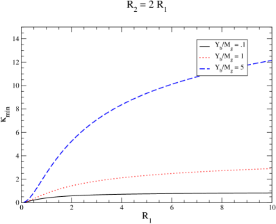
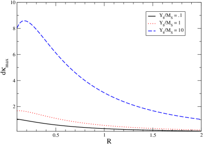
The δκmax𝛿subscript𝜅𝑚𝑎𝑥\delta\kappa_{max} term is 𝒪(1)𝒪1{\cal O}(1) in MEW/MSsubscript𝑀𝐸𝑊subscript𝑀𝑆M_{EW}/M_{S} and has its largest values for small R𝑅R and large ratios of Yb/MSsubscript𝑌𝑏subscript𝑀𝑆Y_{b}/M_{S}, as can be seen in Fig. 2. Large effects can be obtained for Yb/MS10similar-tosubscript𝑌𝑏subscript𝑀𝑆10Y_{b}/M_{S}\sim 10 and Mg~<<MSmuch-less-thansubscript𝑀~𝑔subscript𝑀𝑆M_{\tilde{g}}<<M_{S}. However, the parameters must be carefully tuned so that Ab/MS <1 <subscript𝐴𝑏subscript𝑀𝑆1A_{b}/M_{S}\mathrel{\hbox to0.0pt{\lower 4.0pt\hbox{\hskip 1.0pt$\sim$}\hss}\raise 1.0pt\hbox{$<$}}1 in order not to break colorGunion et al. (1988).
Refer to caption
Figure 2: Contribution of δκmax𝛿subscript𝜅𝑚𝑎𝑥\delta\kappa_{max} defined in Eq. 42 as a function of R=Mg~/MS𝑅subscript𝑀~𝑔subscript𝑀𝑆R=M_{\tilde{g}}/M_{S}.

The amplitude squared, summing over final state spins and colors and averaging over initial state spins and colors, including one-loop SQCD corrections is

|𝒜¯|max2superscriptsubscript¯𝒜𝑚𝑎𝑥2\displaystyle\left|{\overline{\mathcal{A}}}\right|_{max}^{2} =\displaystyle= 2παs(μR)3gbbh2[(u2+Mh4st)[1+2(δgbbhgbbh)max]+αs(μR)2πMh2MS2δκmax].2𝜋subscript𝛼𝑠subscript𝜇𝑅3superscriptsubscript𝑔𝑏𝑏2delimited-[]superscript𝑢2superscriptsubscript𝑀4𝑠𝑡delimited-[]12subscript𝛿subscript𝑔𝑏𝑏subscript𝑔𝑏𝑏𝑚𝑎𝑥subscript𝛼𝑠subscript𝜇𝑅2𝜋superscriptsubscript𝑀2superscriptsubscript𝑀𝑆2𝛿subscript𝜅𝑚𝑎𝑥\displaystyle-\frac{2\pi\alpha_{s}(\mu_{R})}{3}g_{bbh}^{2}\left[\left(\frac{u^{2}+M_{h}^{4}}{st}\right)\left[1+2\biggl{(}{\delta g_{bbh}\over g_{bbh}}\biggr{)}_{max}\right]+{\alpha_{s}(\mu_{R})\over 2\pi}\frac{M_{h}^{2}}{M_{S}^{2}}\delta\kappa_{max}\right]\,. (43)

Note that in the cross section, the δκmax𝛿subscript𝜅𝑚𝑎𝑥\delta\kappa_{max} term is not enhanced by a power of s𝑠s and gives a contribution of 𝒪(MEW2MS2)𝒪superscriptsubscript𝑀𝐸𝑊2superscriptsubscript𝑀𝑆2{\cal O}\biggl{(}{M_{EW}^{2}\over M_{S}^{2}}\biggr{)}.

Expanding ΔbsubscriptΔ𝑏\Delta_{b} in the maximal mixing limit,

Δbαs(μS)3πMg~μMS2tanβf1(R)+𝒪(MEW4MS4).subscriptΔ𝑏subscript𝛼𝑠subscript𝜇𝑆3𝜋subscript𝑀~𝑔𝜇superscriptsubscript𝑀𝑆2𝛽subscript𝑓1𝑅𝒪superscriptsubscript𝑀𝐸𝑊4superscriptsubscript𝑀𝑆4\Delta_{b}\rightarrow-{\alpha_{s}(\mu_{S})\over 3\pi}{M_{\tilde{g}}\mu\over M_{S}^{2}}\tan\beta f_{1}(R)+{\cal O}\biggl{(}{M_{EW}^{4}\over M_{S}^{4}}\biggr{)}\,. (44)

By comparison with Eq. 14,

|𝒜¯|max2superscriptsubscript¯𝒜𝑚𝑎𝑥2\displaystyle\left|{\overline{\mathcal{A}}}\right|_{max}^{2} =\displaystyle= 2παs(μR)3(gbbhΔb)2{(u2+Mh4st)[1+2(δgbbhgbbh)max(2)]\displaystyle-\frac{2\pi\alpha_{s}(\mu_{R})}{3}(g_{bbh}^{\Delta_{b}})^{2}\left\{\left(\frac{u^{2}+M_{h}^{4}}{st}\right)\left[1+2\biggl{(}{\delta g_{bbh}\over g_{bbh}}\biggr{)}^{(2)}_{max}\right]\right. (45)
+αs(μR)2πMh2MS2δκmax}+𝒪([MEWMS]4,αs3).\displaystyle\left.+{\alpha_{s}(\mu_{R})\over 2\pi}\frac{M_{h}^{2}}{M_{S}^{2}}\delta\kappa_{max}\right\}+{\cal O}\biggl{(}\biggl{[}{M_{EW}\over M_{S}}\biggr{]}^{4},\alpha_{s}^{3}\biggr{)}\,.

Note that the mis-match in the arguments of αssubscript𝛼𝑠\alpha_{s} in Eqs. 44 and 45 is higher order in αssubscript𝛼𝑠\alpha_{s} than the terms considered here. The (δgbbh/gbbh)max(2)subscriptsuperscript𝛿subscript𝑔𝑏𝑏subscript𝑔𝑏𝑏2𝑚𝑎𝑥(\delta g_{bbh}/g_{bbh})^{(2)}_{max} and δκmax𝛿subscript𝜅𝑚𝑎𝑥\delta\kappa_{max} terms both correspond to contributions which are not present in the effective Lagrangian approach. These terms are, however, suppressed by powers of MEW2/MS2superscriptsubscript𝑀𝐸𝑊2superscriptsubscript𝑀𝑆2M_{EW}^{2}/M_{S}^{2} and the non-decoupling effects discussed in Refs. Haber et al. (2001) and Guasch et al. (2003) are completely contained in the gbbhΔbsuperscriptsubscript𝑔𝑏𝑏subscriptΔ𝑏g_{bbh}^{\Delta_{b}} term.

III.2 Minimal Mixing in the b𝑏b Squark Sector

The minimal mixing scenario is characterized by a mass splitting between the b𝑏b squarks which is of order the b𝑏b squark mass, Mb~12Mb~22MS2similar-todelimited-∣∣superscriptsubscript𝑀subscript~𝑏12superscriptsubscript𝑀subscript~𝑏22superscriptsubscript𝑀𝑆2\mid M_{\tilde{b}_{1}}^{2}-M_{\tilde{b}_{2}}^{2}\mid\sim M_{S}^{2}. In this case,

m~L2m~R2>>mbXb(1+Δb),much-greater-thandelimited-∣∣superscriptsubscript~𝑚𝐿2superscriptsubscript~𝑚𝑅2subscript𝑚𝑏delimited-∣∣subscript𝑋𝑏1subscriptΔ𝑏\mid{\tilde{m}}_{L}^{2}-{\tilde{m}}_{R}^{2}\mid>>{m_{b}\mid X_{b}\mid\over(1+\Delta_{b})}\,, (46)

and the mixing angle in the b𝑏b squark sector is close to zero,

cos2θ~b12mb2Xb2(Mb~12Mb~22)2(11+Δb)2.similar-to2subscript~𝜃𝑏12superscriptsubscript𝑚𝑏2superscriptsubscript𝑋𝑏2superscriptsuperscriptsubscript𝑀subscript~𝑏12superscriptsubscript𝑀subscript~𝑏222superscript11subscriptΔ𝑏2\cos 2{\tilde{\theta}}_{b}\sim 1-{2m_{b}^{2}X_{b}^{2}\over(M_{{\tilde{b}}_{1}}^{2}-M_{{\tilde{b}}_{2}}^{2})^{2}}\biggl{(}{1\over 1+\Delta_{b}}\biggr{)}^{2}\,. (47)

The non-zero subamplitudes are

Assubscript𝐴𝑠\displaystyle A_{s} =\displaystyle= gsTAgbbhMsμ{1+(δgbbhgbbh)min+αs(μR)4πsM~g2δκmin}subscript𝑔𝑠superscript𝑇𝐴subscript𝑔𝑏𝑏superscriptsubscript𝑀𝑠𝜇1subscript𝛿subscript𝑔𝑏𝑏subscript𝑔𝑏𝑏𝑚𝑖𝑛subscript𝛼𝑠subscript𝜇𝑅4𝜋𝑠superscriptsubscript~𝑀𝑔2𝛿subscript𝜅𝑚𝑖𝑛\displaystyle-g_{s}T^{A}g_{bbh}M_{s}^{\mu}\biggl{\{}1+\biggl{(}{\delta g_{bbh}\over g_{bbh}}\biggr{)}_{min}+{\alpha_{s}(\mu_{R})\over 4\pi}{s\over{\tilde{M}}_{g}^{2}}\delta\kappa_{min}\biggr{\}}
Atsubscript𝐴𝑡\displaystyle A_{t} =\displaystyle= gsTAgbbhMtμ{1+(δgbbhgbbh)min}subscript𝑔𝑠superscript𝑇𝐴subscript𝑔𝑏𝑏superscriptsubscript𝑀𝑡𝜇1subscript𝛿subscript𝑔𝑏𝑏subscript𝑔𝑏𝑏𝑚𝑖𝑛\displaystyle-g_{s}T^{A}g_{bbh}M_{t}^{\mu}\biggl{\{}1+\biggl{(}{\delta g_{bbh}\over g_{bbh}}\biggr{)}_{min}\biggr{\}}
A1subscript𝐴1\displaystyle A_{1} =\displaystyle= gsTAgbbhM1μ(αs(μR)u2πM~g2)δκmin.subscript𝑔𝑠superscript𝑇𝐴subscript𝑔𝑏𝑏superscriptsubscript𝑀1𝜇subscript𝛼𝑠subscript𝜇𝑅𝑢2𝜋superscriptsubscript~𝑀𝑔2𝛿subscript𝜅𝑚𝑖𝑛\displaystyle-g_{s}T^{A}g_{bbh}M_{1}^{\mu}\biggl{(}-{\alpha_{s}(\mu_{R})u\over 2\pi{\tilde{M}}_{g}^{2}}\biggr{)}\delta\kappa_{min}\,. (48)

Expanding the exact one-loop results of Appendix B in the minimal mixing scenario,

δκmin=18Σi=12(Ri2[19f31(Ri)+f3(Ri)])+YbMg~R12R22R22R12(3h1(R1,R2,1)+83h1(R1,R2,2)),𝛿subscript𝜅𝑚𝑖𝑛18superscriptsubscriptΣ𝑖12superscriptsubscript𝑅𝑖2delimited-[]19superscriptsubscript𝑓31subscript𝑅𝑖subscript𝑓3subscript𝑅𝑖subscript𝑌𝑏subscript𝑀~𝑔superscriptsubscript𝑅12superscriptsubscript𝑅22superscriptsubscript𝑅22superscriptsubscript𝑅123subscript1subscript𝑅1subscript𝑅2183subscript1subscript𝑅1subscript𝑅22\delta\kappa_{min}={1\over 8}\Sigma_{i=1}^{2}\biggl{(}R_{i}^{2}\biggl{[}{1\over 9}f_{3}^{-1}(R_{i})+f_{3}(R_{i})\biggr{]}\biggr{)}+{Y_{b}\over M_{\tilde{g}}}{R_{1}^{2}R_{2}^{2}\over R_{2}^{2}-R_{1}^{2}}\biggl{(}3h_{1}(R_{1},R_{2},1)+{8\over 3}h_{1}(R_{1},R_{2},2)\biggr{)}\,, (49)

where Ri=Mg~/Mb~isubscript𝑅𝑖subscript𝑀~𝑔subscript𝑀subscript~𝑏𝑖R_{i}=M_{\tilde{g}}/M_{\tilde{b}_{i}} and the functions fi(Ri)subscript𝑓𝑖subscript𝑅𝑖f_{i}(R_{i}) and hi(R1,R2,n)subscript𝑖subscript𝑅1subscript𝑅2𝑛h_{i}(R_{1},R_{2},n) are defined in Appendix C. The δκmin𝛿subscript𝜅𝑚𝑖𝑛\delta\kappa_{min} function is shown in Fig. 3. For large values of Yb/Mg~subscript𝑌𝑏subscript𝑀~𝑔Y_{b}/M_{\tilde{g}} it can be significantly larger than 111.

Refer to caption
Figure 3: Contribution of δκmin𝛿subscript𝜅𝑚𝑖𝑛\delta\kappa_{min} defined in Eq. 49 as a function of Ri=Mg~/Mb~isubscript𝑅𝑖subscript𝑀~𝑔subscript𝑀subscript~𝑏𝑖R_{i}=M_{\tilde{g}}/M_{{\tilde{b}}_{i}} .

As in the previous section, the spin and color averaged amplitude-squared is,

A¯min2superscriptsubscriptdelimited-∣∣¯𝐴𝑚𝑖𝑛2\displaystyle\mid{\overline{A}}\mid_{min}^{2} =\displaystyle= 2αs(μR)π3(gbbh2){(Mh4+u2)st[1+2(δgbbhgbbh)min]+αs(μR)2πδκminMh2Mg~2},2subscript𝛼𝑠subscript𝜇𝑅𝜋3superscriptsubscript𝑔𝑏𝑏2superscriptsubscript𝑀4superscript𝑢2𝑠𝑡delimited-[]12subscript𝛿subscript𝑔𝑏𝑏subscript𝑔𝑏𝑏𝑚𝑖𝑛subscript𝛼𝑠subscript𝜇𝑅2𝜋𝛿subscript𝜅𝑚𝑖𝑛superscriptsubscript𝑀2superscriptsubscript𝑀~𝑔2\displaystyle-{2\alpha_{s}(\mu_{R})\pi\over 3}(g_{bbh}^{2})\biggl{\{}{(M_{h}^{4}+u^{2})\over st}\biggl{[}1+2\biggl{(}{\delta g_{bbh}\over g_{bbh}}\biggr{)}_{min}\biggr{]}+{\alpha_{s}(\mu_{R})\over 2\pi}\delta\kappa_{min}{M_{h}^{2}\over M_{\tilde{g}}^{2}}\biggr{\}}\,, (50)

with,

(δgbbhgbbh)min=(δgbbhgbbh)min(1)+(δgbbhgbbh)min(2).subscript𝛿subscript𝑔𝑏𝑏subscript𝑔𝑏𝑏𝑚𝑖𝑛subscriptsuperscript𝛿subscript𝑔𝑏𝑏subscript𝑔𝑏𝑏1𝑚𝑖𝑛subscriptsuperscript𝛿subscript𝑔𝑏𝑏subscript𝑔𝑏𝑏2𝑚𝑖𝑛\biggl{(}{\delta g_{bbh}\over g_{bbh}}\biggr{)}_{min}=\biggl{(}{\delta g_{bbh}\over g_{bbh}}\biggr{)}^{(1)}_{min}+\biggl{(}{\delta g_{bbh}\over g_{bbh}}\biggr{)}^{(2)}_{min}\,. (51)

The leading order term in MEW/MSsubscript𝑀𝐸𝑊subscript𝑀𝑆M_{EW}/M_{S} is 𝒪(1)𝒪1{\cal O}(1),

(δgbbhgbbh)min(1)=2αs(μR)3π(XbYb)Mg~R12R22R12R22h1(R1,R2,0).subscriptsuperscript𝛿subscript𝑔𝑏𝑏subscript𝑔𝑏𝑏1𝑚𝑖𝑛2subscript𝛼𝑠subscript𝜇𝑅3𝜋subscript𝑋𝑏subscript𝑌𝑏subscript𝑀~𝑔superscriptsubscript𝑅12superscriptsubscript𝑅22superscriptsubscript𝑅12superscriptsubscript𝑅22subscript1subscript𝑅1subscript𝑅20\biggl{(}{\delta g_{bbh}\over g_{bbh}}\biggr{)}^{(1)}_{min}={2\alpha_{s}(\mu_{R})\over 3\pi}{(X_{b}-Y_{b})\over M_{\tilde{g}}}{R_{1}^{2}R_{2}^{2}\over R_{1}^{2}-R_{2}^{2}}h_{1}(R_{1},R_{2},0)\,. (52)

The subleading terms are 𝒪(MEW2MS2)𝒪superscriptsubscript𝑀𝐸𝑊2superscriptsubscript𝑀𝑆2{\cal O}\biggl{(}{M_{EW}^{2}\over M_{S}^{2}}\biggr{)},

(δgbbhgbbh)min(2)subscriptsuperscript𝛿subscript𝑔𝑏𝑏subscript𝑔𝑏𝑏2𝑚𝑖𝑛\displaystyle\biggl{(}{\delta g_{bbh}\over g_{bbh}}\biggr{)}^{(2)}_{min} =\displaystyle= αs4π{8Mg~Yb3ΔMb~122[h2(R1,R2)Mh2ΔMb~122\displaystyle{\alpha_{s}\over 4\pi}\biggl{\{}-\frac{8M_{\tilde{g}}Y_{b}}{3\Delta M_{\tilde{b}_{12}}^{2}}\left[\frac{h_{2}\left(R_{1},R_{2}\right)M_{h}^{2}}{\Delta M_{\tilde{b}_{12}}^{2}}\right. (53)
+mb2Xb2(ΔMb~122)2(1+Δb)2{2𝒮(f1(R)Mb~2)+h1(R1,R2,0)ΔMb~122}]\displaystyle\left.\left.+\frac{m_{b}^{2}X_{b}^{2}}{\left(\Delta M_{\tilde{b}_{12}}^{2}\right)^{2}(1+\Delta_{b})^{2}}\left\{2\mathcal{S}\left(\frac{f_{1}\left(R\right)}{M_{\tilde{b}}^{2}}\right)\right.\right.\left.+\frac{h_{1}\left(R_{1},R_{2},0\right)}{\Delta M_{\tilde{b}_{12}}^{2}}\right\}\right]
+43cβsα+βsαI3bMZ2[𝒮(3f1(R)f2(R)3Mb~2)2Mg~XbΔMb~122𝒜(f1(R)Mb~2)]43subscript𝑐𝛽subscript𝑠𝛼𝛽subscript𝑠𝛼superscriptsubscript𝐼3𝑏superscriptsubscript𝑀𝑍2delimited-[]𝒮3subscript𝑓1𝑅subscript𝑓2𝑅3superscriptsubscript𝑀~𝑏22subscript𝑀~𝑔subscript𝑋𝑏Δsuperscriptsubscript𝑀subscript~𝑏122𝒜subscript𝑓1𝑅superscriptsubscript𝑀~𝑏2\displaystyle+\frac{4}{3}\frac{c_{\beta}s_{\alpha+\beta}}{s_{\alpha}}I_{3}^{b}M_{Z}^{2}\left[\mathcal{S}\left(\frac{3f_{1}\left(R\right)-f_{2}\left(R\right)}{3M_{\tilde{b}}^{2}}\right)-\frac{2M_{\tilde{g}}X_{b}}{\Delta M_{\tilde{b}_{12}}^{2}}\mathcal{A}\left(\frac{f_{1}\left(R\right)}{M_{\tilde{b}}^{2}}\right)\right]
+43cβsα+βsα(I3b2QbsW2)MZ2[𝒜(3f1(R)f2(R)3Mb~2)\displaystyle+\frac{4}{3}\frac{c_{\beta}s_{\alpha+\beta}}{s_{\alpha}}\left(I_{3}^{b}-2Q^{b}s_{W}^{2}\right)M_{Z}^{2}\left[\mathcal{A}\left(\frac{3f_{1}\left(R\right)-f_{2}\left(R\right)}{3M_{\tilde{b}}^{2}}\right)\right.
2Mg~XbΔMb~122{𝒮(f1(R)Mb~2)+h1(R1,R2,0)ΔMb~122}]\displaystyle\left.-\frac{2M_{\tilde{g}}X_{b}}{\Delta M_{\tilde{b}_{12}}^{2}}\left\{\mathcal{S}\left(\frac{f_{1}\left(R\right)}{M_{\tilde{b}}^{2}}\right)+\frac{h_{1}\left(R_{1},R_{2},0\right)}{\Delta M_{\tilde{b}_{12}}^{2}}\right\}\right]
+83mb2XbYbΔMb~122(1+Δb)2𝒜(3f1(R)f2(R)3Mb~2)}.\displaystyle+\frac{8}{3}\frac{m_{b}^{2}X_{b}Y_{b}}{\Delta M_{\tilde{b}_{12}}^{2}(1+\Delta_{b})^{2}}\mathcal{A}\left(\frac{3f_{1}\left(R\right)-f_{2}\left(R\right)}{3M_{\tilde{b}}^{2}}\right)\biggr{\}}\,.

The symmetric and anti-symmetric functions are defined,

𝒮(f(R,Mb~)\displaystyle{\mathcal{S}}(f(R,M_{\tilde{b}}) \displaystyle\equiv 12[f(R1,Mb~1)+f(R2,Mb~2)]12delimited-[]𝑓subscript𝑅1subscript𝑀subscript~𝑏1𝑓subscript𝑅2subscript𝑀subscript~𝑏2\displaystyle{1\over 2}\biggl{[}f(R_{1},M_{{\tilde{b}}_{1}})+f(R_{2},M_{{\tilde{b}}_{2}})\biggr{]}
𝒜(f(R,Mb~)\displaystyle{\mathcal{A}}(f(R,M_{\tilde{b}}) \displaystyle\equiv 12[f(R1,Mb~1)f(R2,Mb~2)]12delimited-[]𝑓subscript𝑅1subscript𝑀subscript~𝑏1𝑓subscript𝑅2subscript𝑀subscript~𝑏2\displaystyle{1\over 2}\biggl{[}f(R_{1},M_{{\tilde{b}}_{1}})-f(R_{2},M_{{\tilde{b}}_{2}})\biggr{]} (54)

and ΔMb~122Mb~12Mb~22Δsubscriptsuperscript𝑀2subscript~𝑏12superscriptsubscript𝑀subscript~𝑏12superscriptsubscript𝑀subscript~𝑏22\Delta M^{2}_{{\tilde{b}}_{12}}\equiv M_{\tilde{b}_{1}}^{2}-M_{\tilde{b}_{2}}^{2}. The remaining functions are defined in Appendix C.

By expanding ΔbsubscriptΔ𝑏\Delta_{b} in the minimal mixing limit, we find the analogous result to that of the maximal mixing case,

A¯min2superscriptsubscriptdelimited-∣∣¯𝐴𝑚𝑖𝑛2\displaystyle\mid{\overline{A}}\mid_{min}^{2} =\displaystyle= 2αsπ3(gbbhΔb)2{(Mh4+u2)st[1+2(δgbbhgbbh)min(2)]\displaystyle-{2\alpha_{s}\pi\over 3}(g_{bbh}^{\Delta_{b}})^{2}\biggl{\{}{(M_{h}^{4}+u^{2})\over st}\biggl{[}1+2\biggl{(}{\delta g_{bbh}\over g_{bbh}}\biggr{)}^{(2)}_{min}\biggr{]} (55)
+αs2πδκminMh2Mg~2}+𝒪([MEWMS]4,αs3).\displaystyle+{\alpha_{s}\over 2\pi}\delta\kappa_{min}{M_{h}^{2}\over M_{\tilde{g}}^{2}}\biggr{\}}+{\cal O}\biggl{(}\biggl{[}{M_{EW}\over M_{S}}\biggr{]}^{4},\alpha_{s}^{3}\biggr{)}\,.

The contributions which are not contained in σIBAsubscript𝜎𝐼𝐵𝐴\sigma_{IBA} are again found to be suppressed by 𝒪([MEWMS]2)𝒪superscriptdelimited-[]subscript𝑀𝐸𝑊subscript𝑀𝑆2{\cal O}\biggl{(}\biggl{[}{M_{EW}\over M_{S}}\biggr{]}^{2}\biggr{)}.

IV Numerical Results

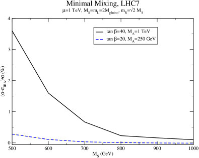
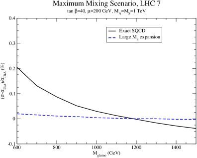
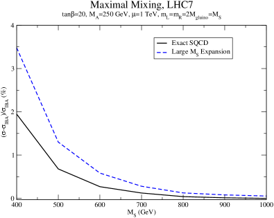
We present results for ppb(b¯)h𝑝𝑝𝑏¯𝑏pp\rightarrow b({\overline{b}})h at s=7TeV𝑠7𝑇𝑒𝑉\sqrt{s}=7~{}TeV with pTb>20GeVsubscript𝑝𝑇𝑏20𝐺𝑒𝑉p_{Tb}>20~{}GeV and ηb<2.0delimited-∣∣subscript𝜂𝑏2.0\mid\eta_{b}\mid<2.0. We use FeynHiggs to generate Mhsubscript𝑀M_{h} and sinαeffsubscript𝛼𝑒𝑓𝑓\sin\alpha_{eff} and then iteratively solve for the b𝑏b squark masses and ΔbsubscriptΔ𝑏\Delta_{b} from Eqs. 12 and 19. We evaluate the 2-loop MS¯¯𝑀𝑆{\overline{MS}} b𝑏b mass at μR=Mh/2subscript𝜇𝑅subscript𝑀2\mu_{R}=M_{h}/2, which we also take to be the renormalization and factorization scales999ΔbsubscriptΔ𝑏\Delta_{b} is evaluated using αs(MS)subscript𝛼𝑠subscript𝑀𝑆\alpha_{s}(M_{S}).. Finally, Figs 4, 5, 6, and 7 use the CTEQ6m NLO parton distribution functionsNadolsky et al. (2008). Figs. 4, 5 and 6 show the percentage deviation of the complete one-loop SQCD calculation from the Improved Born Approximation of Eq. 16 for tanβ=40𝛽40\tan\beta=40 and tanβ=20𝛽20\tan\beta=20 and representative values of the MSSM parameters101010Figs. 4, 5 and 6 do not include the pure QCD NLO correctionsDicus et al. (1999).. In both extremes of b𝑏b squark mixing, the Improved Born Approximation approximation is within a few percent of the complete one-loop SQCD calculation and so is a reliable prediction for the rate. This is true for both large and small MAsubscript𝑀𝐴M_{A}. In addition, the large MSsubscript𝑀𝑆M_{S} expansion accurately reproduces the full SQCD one-loop result to within a few percent. These results are expected from the expansions of Eqs. 45 and 55, since the terms which differ between the Improved Born Approximation and the one-loop calculation are suppressed in the large MSsubscript𝑀𝑆M_{S} limit.

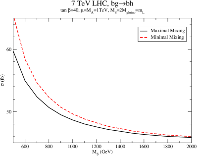
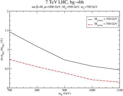
Fig. 7 compares the total SQCD rate for maximal and minimal mixing, which bracket the allowed mixing possibilities. For large MSsubscript𝑀𝑆M_{S}, the effect of the mixing is quite small, while for MS800GeVsimilar-tosubscript𝑀𝑆800𝐺𝑒𝑉M_{S}\sim 800~{}GeV, the mixing effects are at most a few fb𝑓𝑏fb. The accuracy of the Improved Born Approximation as a function of mRsubscript𝑚𝑅m_{R} is shown in Fig. 8 for fixed MA,μsubscript𝑀𝐴𝜇M_{A},\mu, and mLsubscript𝑚𝐿m_{L}. As mRsubscript𝑚𝑅m_{R} is increased, the effects become very tiny. Even for light gluino masses, the Improved Born Approximation reproduces the exact SQCD result to within a few percent.
Refer to caption
Figure 4: Percentage difference between the Improved Born Approximation and the exact one-loop SQCD calculation of ppbh𝑝𝑝𝑏pp\rightarrow bh for maximal mixing in the b𝑏b-squark sector at s=7TeV𝑠7𝑇𝑒𝑉\sqrt{s}=7~{}TeV, tanβ=40𝛽40\tan\beta=40, and MA=1TeVsubscript𝑀𝐴1𝑇𝑒𝑉M_{A}=1~{}TeV.
Refer to caption
Figure 5: Percentage difference between the Improved Born Approximation and the exact one-loop SQCD calculation of ppbh𝑝𝑝𝑏pp\rightarrow bh for maximal mixing in the b𝑏b-squark sector at s=7TeV𝑠7𝑇𝑒𝑉\sqrt{s}=7~{}TeV, tanβ=20𝛽20\tan\beta=20, and MA=250GeVsubscript𝑀𝐴250𝐺𝑒𝑉M_{A}=250~{}GeV.
Refer to caption
Figure 6: Percentage difference between the Improved Born Approximation and the exact one-loop SQCD calculation for ppbh𝑝𝑝𝑏pp\rightarrow bh for minimal mixing in the b𝑏b squark sector at s=7TeV𝑠7𝑇𝑒𝑉\sqrt{s}=7~{}TeV.
Refer to caption
Figure 7: Comparison between the exact one-loop SQCD calculation for ppbh𝑝𝑝𝑏pp\rightarrow bh for minimal and maximal mixing in the b𝑏b squark sector at s=7TeV𝑠7𝑇𝑒𝑉\sqrt{s}=7~{}TeV and tanβ=40𝛽40\tan\beta=40. The minimal mixing curve has mR=2MSsubscript𝑚𝑅2subscript𝑀𝑆m_{R}=\sqrt{2}M_{S} and θ~b0similar-tosubscript~𝜃𝑏0{\tilde{\theta}}_{b}\sim 0, while the maximal mixing curve has mR=MSsubscript𝑚𝑅subscript𝑀𝑆m_{R}=M_{S} and θ~bπ4similar-tosubscript~𝜃𝑏𝜋4{\tilde{\theta}}_{b}\sim{\pi\over 4}.
Refer to caption
Figure 8: Percentage difference between the Improved Born Approximation and the exact one-loop SQCD calculation for ppbh𝑝𝑝𝑏pp\rightarrow bh as a function of mRsubscript𝑚𝑅m_{R} at s=7TeV𝑠7𝑇𝑒𝑉\sqrt{s}=7~{}TeV and tanβ=40𝛽40\tan\beta=40.
Refer to caption
Figure 9: Total cross section for ppb(b¯)h𝑝𝑝𝑏¯𝑏pp\rightarrow b(\overline{b})h production including NLO QCD and SQCD corrections (dotted lines) as a function of renormalization/factorization scale using CTEQ6m (black) and MSTW2008 NLO (red) PDFs. We take Mg~=1TeVsubscript𝑀~𝑔1𝑇𝑒𝑉M_{\tilde{g}}=1~{}TeV and the remaining MSSM parameters as in Fig. 4.

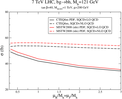
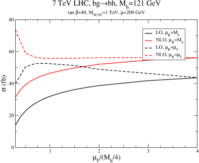
In Fig. 9, we show the scale dependence for the total rate, including NLO QCD and SQCD corrections (dotted lines) for a representative set of MSSM parameters at s=7TeV𝑠7𝑇𝑒𝑉\sqrt{s}=7~{}TeV. The NLO scale dependence is quite small when μR=μFMhsubscript𝜇𝑅subscript𝜇𝐹similar-tosubscript𝑀\mu_{R}=\mu_{F}\sim M_{h}. However, there is a roughly 5%similar-toabsentpercent5\sim 5\% difference between the predictions found using the CTEQ6m PDFs and the MSTW2008 NLO PDFsMartin et al. (2009). In Fig. 10, we show the scale dependence for small μFsubscript𝜇𝐹\mu_{F} (as preferred by Maltoni et al. (2005)), and see that it is significantly larger than in Fig. 9. This is consistent with the results of Harlander and Kilgore (2003); Dittmaier et al. (2011).
Refer to caption
Figure 10: Total cross section for ppb(b¯)h𝑝𝑝𝑏¯𝑏pp\rightarrow b(\overline{b})h production including NLO QCD and SQCD corrections as a function of the factorization scale using MSTW2008 NLO PDFs. We take Mg~=1TeVsubscript𝑀~𝑔1𝑇𝑒𝑉M_{\tilde{g}}=1~{}TeV and the remaining MSSM parameters as in Fig. 4.

V Conclusion

Our major results are the analytic expressions for the SQCD corrections to b𝑏b Higgs associated production in the minimal (Eqs.  41, 42 and 45) and maximal (Eqs. 49, 53 and 55) b𝑏b squark mixing scenarios for large tanβ𝛽\tan\beta and squark masses,MSsubscript𝑀𝑆M_{S}. These results clearly demonstrate that deviations from the ΔbsubscriptΔ𝑏\Delta_{b} approximation are suppressed by powers of (MEW/MS)subscript𝑀𝐸𝑊subscript𝑀𝑆(M_{EW}/M_{S}) in the large tanβ𝛽\tan\beta region. The ΔbsubscriptΔ𝑏\Delta_{b} approximation hence yields an accurate prediction in the 555 flavor number scheme for the cross section for squark and gluino masses at the TeV𝑇𝑒𝑉TeV scale. As a by-product of our calculation, we update the predictions for b𝑏b Higgs production at s=7TeV𝑠7𝑇𝑒𝑉\sqrt{s}=7~{}TeV.

Acknowledgements

S. Dawson  and P.Jaiswal are supported by the United States Department of Energy under Grant DE-AC02-98CH10886.

Appendix A: Passarino-Veltman Functions

The scalar integrals are defined as:

i16π2A0(M02)𝑖16superscript𝜋2subscript𝐴0superscriptsubscript𝑀02\displaystyle{i\over 16\pi^{2}}A_{0}(M_{0}^{2}) =\displaystyle= dnk(2π)n1N0,superscript𝑑𝑛𝑘superscript2𝜋𝑛1subscript𝑁0\displaystyle\int\frac{d^{n}k}{(2\pi)^{n}}\frac{1}{N_{0}}\,,
i16π2B0(p12;M02,M12)𝑖16superscript𝜋2subscript𝐵0superscriptsubscript𝑝12superscriptsubscript𝑀02superscriptsubscript𝑀12\displaystyle{i\over 16\pi^{2}}B_{0}(p_{1}^{2};M_{0}^{2},M_{1}^{2}) =\displaystyle= dnk(2π)n1N0N1,superscript𝑑𝑛𝑘superscript2𝜋𝑛1subscript𝑁0subscript𝑁1\displaystyle\int\frac{d^{n}k}{(2\pi)^{n}}\frac{1}{N_{0}N_{1}}\,,
i16π2C0(p12,p22,(p1+p2)2;M02,M12,M22)𝑖16superscript𝜋2subscript𝐶0superscriptsubscript𝑝12superscriptsubscript𝑝22superscriptsubscript𝑝1subscript𝑝22superscriptsubscript𝑀02superscriptsubscript𝑀12superscriptsubscript𝑀22\displaystyle{i\over 16\pi^{2}}C_{0}(p_{1}^{2},p_{2}^{2},(p_{1}+p_{2})^{2};M_{0}^{2},M_{1}^{2},M_{2}^{2}) =\displaystyle= dnk(2π)n1N0N1N2,superscript𝑑𝑛𝑘superscript2𝜋𝑛1subscript𝑁0subscript𝑁1subscript𝑁2\displaystyle\int\frac{d^{n}k}{(2\pi)^{n}}\frac{1}{N_{0}N_{1}N_{2}}\,,
i16π2D0(p12,p22,p32,p42,(p1+p2)2,(p2+p3)2;M02,M12,M22,M32)𝑖16superscript𝜋2subscript𝐷0superscriptsubscript𝑝12superscriptsubscript𝑝22superscriptsubscript𝑝32superscriptsubscript𝑝42superscriptsubscript𝑝1subscript𝑝22superscriptsubscript𝑝2subscript𝑝32superscriptsubscript𝑀02superscriptsubscript𝑀12superscriptsubscript𝑀22superscriptsubscript𝑀32\displaystyle{i\over 16\pi^{2}}D_{0}(p_{1}^{2},p_{2}^{2},p_{3}^{2},p_{4}^{2},(p_{1}+p_{2})^{2},(p_{2}+p_{3})^{2};M_{0}^{2},M_{1}^{2},M_{2}^{2},M_{3}^{2})
=dnk(2π)n1N0N1N2N3,absentsuperscript𝑑𝑛𝑘superscript2𝜋𝑛1subscript𝑁0subscript𝑁1subscript𝑁2subscript𝑁3\displaystyle\qquad\qquad\qquad=\int\frac{d^{n}k}{(2\pi)^{n}}\frac{1}{N_{0}N_{1}N_{2}N_{3}}\,, (56)

where,

N0subscript𝑁0\displaystyle N_{0} =\displaystyle= k2M02superscript𝑘2superscriptsubscript𝑀02\displaystyle k^{2}-M_{0}^{2}
N1subscript𝑁1\displaystyle N_{1} =\displaystyle= (k+p1)2M12superscript𝑘subscript𝑝12superscriptsubscript𝑀12\displaystyle(k+p_{1})^{2}-M_{1}^{2}
N2subscript𝑁2\displaystyle N_{2} =\displaystyle= (k+p1+p2)2M22superscript𝑘subscript𝑝1subscript𝑝22superscriptsubscript𝑀22\displaystyle(k+p_{1}+p_{2})^{2}-M_{2}^{2}
N3subscript𝑁3\displaystyle N_{3} =\displaystyle= (k+p1+p2+p3)2M32.superscript𝑘subscript𝑝1subscript𝑝2subscript𝑝32superscriptsubscript𝑀32\displaystyle(k+p_{1}+p_{2}+p_{3})^{2}-M_{3}^{2}\,. (57)

The tensor integrals encountered are expanded in terms of the external momenta pisubscript𝑝𝑖p_{i} and the metric tensor gμνsuperscript𝑔𝜇𝜈g^{\mu\nu}. For the two-point function we write:

i16π2Bμ(p12;M02,M12)𝑖16superscript𝜋2superscript𝐵𝜇superscriptsubscript𝑝12superscriptsubscript𝑀02superscriptsubscript𝑀12\displaystyle{i\over 16\pi^{2}}B^{\mu}(p_{1}^{2};M_{0}^{2},M_{1}^{2}) =\displaystyle= dnk(2π)nkμN0N1superscript𝑑𝑛𝑘superscript2𝜋𝑛superscript𝑘𝜇subscript𝑁0subscript𝑁1\displaystyle\int\frac{d^{n}k}{(2\pi)^{n}}\frac{k^{\mu}}{N_{0}N_{1}} (58)
\displaystyle\equiv i16π2p1μB1(p12,M02,M12),𝑖16superscript𝜋2superscriptsubscript𝑝1𝜇subscript𝐵1superscriptsubscript𝑝12superscriptsubscript𝑀02superscriptsubscript𝑀12\displaystyle{i\over 16\pi^{2}}p_{1}^{\mu}B_{1}(p_{1}^{2},M_{0}^{2},M_{1}^{2})\,,

while for the three-point functions we have both rank-one and rank-two tensor integrals which we expand as:

Cμ(p12,p22,(p1+p2)2;M02,M12,M22)superscript𝐶𝜇superscriptsubscript𝑝12superscriptsubscript𝑝22superscriptsubscript𝑝1subscript𝑝22superscriptsubscript𝑀02superscriptsubscript𝑀12superscriptsubscript𝑀22\displaystyle C^{\mu}(p_{1}^{2},p_{2}^{2},(p_{1}+p_{2})^{2};M_{0}^{2},M_{1}^{2},M_{2}^{2}) =\displaystyle= p1μC11+p2μC12,superscriptsubscript𝑝1𝜇subscript𝐶11superscriptsubscript𝑝2𝜇subscript𝐶12\displaystyle p_{1}^{\mu}C_{11}+p_{2}^{\mu}C_{12}\,,
Cμν(p12,p22,(p1+p2)2;M02,M12,M22)superscript𝐶𝜇𝜈superscriptsubscript𝑝12superscriptsubscript𝑝22superscriptsubscript𝑝1subscript𝑝22superscriptsubscript𝑀02superscriptsubscript𝑀12superscriptsubscript𝑀22\displaystyle C^{\mu\nu}(p_{1}^{2},p_{2}^{2},(p_{1}+p_{2})^{2};M_{0}^{2},M_{1}^{2},M_{2}^{2}) =\displaystyle= p1μp1νC21+p2μp2νC22superscriptsubscript𝑝1𝜇superscriptsubscript𝑝1𝜈subscript𝐶21superscriptsubscript𝑝2𝜇superscriptsubscript𝑝2𝜈subscript𝐶22\displaystyle p_{1}^{\mu}p_{1}^{\nu}C_{21}+p_{2}^{\mu}p_{2}^{\nu}C_{22} (59)
+\displaystyle+ (p1μp2ν+p1νp2μ)C23+gμνC24,superscriptsubscript𝑝1𝜇superscriptsubscript𝑝2𝜈superscriptsubscript𝑝1𝜈superscriptsubscript𝑝2𝜇subscript𝐶23superscript𝑔𝜇𝜈subscript𝐶24\displaystyle(p_{1}^{\mu}p_{2}^{\nu}+p_{1}^{\nu}p_{2}^{\mu})C_{23}+g^{\mu\nu}C_{24}\,,

where:

i16π2Cμ(Cμν)(p12,p22,(p1+p2)2;M02,M12,M22)dnk(2π)nkμ(kμkν)N0N1N2𝑖16superscript𝜋2superscript𝐶𝜇superscript𝐶𝜇𝜈superscriptsubscript𝑝12superscriptsubscript𝑝22superscriptsubscript𝑝1subscript𝑝22superscriptsubscript𝑀02superscriptsubscript𝑀12superscriptsubscript𝑀22superscript𝑑𝑛𝑘superscript2𝜋𝑛superscript𝑘𝜇superscript𝑘𝜇superscript𝑘𝜈subscript𝑁0subscript𝑁1subscript𝑁2{i\over 16\pi^{2}}C^{\mu}(C^{\mu\nu})(p_{1}^{2},p_{2}^{2},(p_{1}+p_{2})^{2};M_{0}^{2},M_{1}^{2},M_{2}^{2})\equiv\int\frac{d^{n}k}{(2\pi)^{n}}\frac{k^{\mu}(k^{\mu}k^{\nu})}{N_{0}N_{1}N_{2}} (60)

Finally, for the box diagrams, we encounter rank-one and rank-two tensor integrals which are written in terms of the Passarino-Veltmann coefficients as:

i16π2Dμ(p12,p22,p32,p42,(p1+p2)2,(p2+p3)2;M02,M12,M22)𝑖16superscript𝜋2superscript𝐷𝜇superscriptsubscript𝑝12superscriptsubscript𝑝22superscriptsubscript𝑝32superscriptsubscript𝑝42superscriptsubscript𝑝1subscript𝑝22superscriptsubscript𝑝2𝑝32superscriptsubscript𝑀02superscriptsubscript𝑀12superscriptsubscript𝑀22\displaystyle{i\over 16\pi^{2}}D^{\mu}(p_{1}^{2},p_{2}^{2},p_{3}^{2},p_{4}^{2},(p_{1}+p_{2})^{2},(p_{2}+p3)^{2};M_{0}^{2},M_{1}^{2},M_{2}^{2}) \displaystyle\equiv dnk(2π)nkμN0N1N2N3superscript𝑑𝑛𝑘superscript2𝜋𝑛superscript𝑘𝜇subscript𝑁0subscript𝑁1subscript𝑁2subscript𝑁3\displaystyle\int\frac{d^{n}k}{(2\pi)^{n}}\frac{k^{\mu}}{N_{0}N_{1}N_{2}N_{3}}
=i16π2{p1μD11+p2μD12+p3μD13}.absent𝑖16superscript𝜋2superscriptsubscript𝑝1𝜇subscript𝐷11superscriptsubscript𝑝2𝜇subscript𝐷12superscriptsubscript𝑝3𝜇subscript𝐷13\displaystyle\qquad\qquad\qquad={i\over 16\pi^{2}}\biggl{\{}p_{1}^{\mu}D_{11}+p_{2}^{\mu}D_{12}+p_{3}^{\mu}D_{13}\biggr{\}}\,. (61)
i16π2Dμν(p12,p22,p32,p42,(p1+p2)2,(p2+p3)2;M02,M12,M22)𝑖16superscript𝜋2superscript𝐷𝜇𝜈superscriptsubscript𝑝12superscriptsubscript𝑝22superscriptsubscript𝑝32superscriptsubscript𝑝42superscriptsubscript𝑝1subscript𝑝22superscriptsubscript𝑝2subscript𝑝32superscriptsubscript𝑀02superscriptsubscript𝑀12superscriptsubscript𝑀22\displaystyle{i\over 16\pi^{2}}D^{\mu\nu}(p_{1}^{2},p_{2}^{2},p_{3}^{2},p_{4}^{2},(p_{1}+p_{2})^{2},(p_{2}+p_{3})^{2};M_{0}^{2},M_{1}^{2},M_{2}^{2}) \displaystyle\equiv dnk(2π)nkμkνN0N1N2N3superscript𝑑𝑛𝑘superscript2𝜋𝑛superscript𝑘𝜇superscript𝑘𝜈subscript𝑁0subscript𝑁1subscript𝑁2subscript𝑁3\displaystyle\int\frac{d^{n}k}{(2\pi)^{n}}\frac{k^{\mu}k^{\nu}}{N_{0}N_{1}N_{2}N_{3}}
=i16π2{gμνD00+tensor structures not needed here}.absent𝑖16superscript𝜋2superscript𝑔𝜇𝜈subscript𝐷00tensor structures not needed here\displaystyle\quad\qquad\qquad={i\over 16\pi^{2}}\biggl{\{}g^{\mu\nu}D_{00}+{\hbox{tensor structures not needed here}}\biggr{\}}\,. (62)

Appendix B: One-Loop Results

In this appendix we give the non-zero contributions of the individual diagrams in terms of the basis functions of Eq. 20 and the decompositions of Eq. 22. The contributions proportional to mbtanβsubscript𝑚𝑏𝛽m_{b}\tan\beta are new and were not included in the results of Ref.Dawson and Jackson (2008). Although we specialize to the case of the lightest Higgs boson, hh, our results are easily generalized to the heavier neutral Higgs boson, H𝐻H, and so the Feynman diagrams in this appendix are shown for ϕi=h,Hsubscriptitalic-ϕ𝑖𝐻\phi_{i}=h,H.

The self-energy diagrams of Fig. 11:

Refer to caption
Refer to caption
Figure 11: Self-energy diagrams, S1subscript𝑆1S_{1} and S2subscript𝑆2S_{2}.
XS1(t)superscriptsubscript𝑋subscript𝑆1𝑡\displaystyle X_{S_{1}}^{\left(t\right)} =\displaystyle= 43i=12{B1(1)i2mbMg~s2b~tB0}(Mb~i2)43superscriptsubscript𝑖12subscript𝐵1superscript1𝑖2subscript𝑚𝑏subscript𝑀~𝑔subscript𝑠2~𝑏𝑡subscript𝐵0superscriptsubscript𝑀subscript~𝑏𝑖2\displaystyle\frac{4}{3}\sum_{i=1}^{2}\left\{B_{1}-\left(-1\right)^{i}\frac{2m_{b}M_{\tilde{g}}s_{2\tilde{b}}}{t}B_{0}\right\}\left(M_{\tilde{b}_{i}}^{2}\right)
XS1(2)superscriptsubscript𝑋subscript𝑆12\displaystyle X_{S_{1}}^{\left(2\right)} =\displaystyle= 43i=12(1)imbMg~s2b~tB0(Mb~i2)43superscriptsubscript𝑖12superscript1𝑖subscript𝑚𝑏subscript𝑀~𝑔subscript𝑠2~𝑏𝑡subscript𝐵0superscriptsubscript𝑀subscript~𝑏𝑖2\displaystyle-\frac{4}{3}\sum_{i=1}^{2}\left(-1\right)^{i}\frac{m_{b}M_{\tilde{g}}s_{2\tilde{b}}}{t}B_{0}\left(M_{\tilde{b}_{i}}^{2}\right) (63)

where we have have used the shorthand notation for the arguments of Passarino-Veltman functions, B0,1(Mb~i2)B0,1(t;Mg~2,Mb~i2)subscript𝐵01superscriptsubscript𝑀subscript~𝑏𝑖2subscript𝐵01𝑡superscriptsubscript𝑀~𝑔2superscriptsubscript𝑀subscript~𝑏𝑖2B_{0,1}\left(M_{\tilde{b}_{i}}^{2}\right)\equiv B_{0,1}\left(t;M_{\tilde{g}}^{2},M_{\tilde{b}_{i}}^{2}\right).

XS2(s)superscriptsubscript𝑋subscript𝑆2𝑠\displaystyle X_{S_{2}}^{\left(s\right)} =\displaystyle= 43i=12{B1(1)i2mbMg~s2b~sB0}(Mb~i2)43superscriptsubscript𝑖12subscript𝐵1superscript1𝑖2subscript𝑚𝑏subscript𝑀~𝑔subscript𝑠2~𝑏𝑠subscript𝐵0superscriptsubscript𝑀subscript~𝑏𝑖2\displaystyle\frac{4}{3}\sum_{i=1}^{2}\left\{B_{1}-\left(-1\right)^{i}\frac{2m_{b}M_{\tilde{g}}s_{2\tilde{b}}}{s}B_{0}\right\}\left(M_{\tilde{b}_{i}}^{2}\right)
XS2(2)superscriptsubscript𝑋subscript𝑆22\displaystyle X_{S_{2}}^{\left(2\right)} =\displaystyle= 43i=12(1)imbMg~s2b~sB0(Mb~i2)43superscriptsubscript𝑖12superscript1𝑖subscript𝑚𝑏subscript𝑀~𝑔subscript𝑠2~𝑏𝑠subscript𝐵0superscriptsubscript𝑀subscript~𝑏𝑖2\displaystyle-\frac{4}{3}\sum_{i=1}^{2}\left(-1\right)^{i}\frac{m_{b}M_{\tilde{g}}s_{2\tilde{b}}}{s}B_{0}\left(M_{\tilde{b}_{i}}^{2}\right) (64)

and B0,1(Mb~i2)B0,1(s;Mg~2,Mb~i2)subscript𝐵01superscriptsubscript𝑀subscript~𝑏𝑖2subscript𝐵01𝑠superscriptsubscript𝑀~𝑔2superscriptsubscript𝑀subscript~𝑏𝑖2B_{0,1}\left(M_{\tilde{b}_{i}}^{2}\right)\equiv B_{0,1}\left(s;M_{\tilde{g}}^{2},M_{\tilde{b}_{i}}^{2}\right)

The vertex functions of Fig. 12:

Refer to caption
Refer to caption
Figure 12: Virtual diagrams, V1subscript𝑉1V_{1} and V2subscript𝑉2V_{2}.

Diagram V1subscript𝑉1V_{1}:

XV1(s)superscriptsubscript𝑋subscript𝑉1𝑠\displaystyle X_{V_{1}}^{\left(s\right)} =\displaystyle= s6i=12{C12+C23(1)i2mbMg~s2b~t(C0+C11)}(Mbi~2)𝑠6superscriptsubscript𝑖12subscript𝐶12subscript𝐶23superscript1𝑖2subscript𝑚𝑏subscript𝑀~𝑔subscript𝑠2~𝑏𝑡subscript𝐶0subscript𝐶11superscriptsubscript𝑀~subscript𝑏𝑖2\displaystyle\frac{s}{6}\sum_{i=1}^{2}\left\{C_{12}+C_{23}-\left(-1\right)^{i}\frac{2m_{b}M_{\tilde{g}}s_{2\tilde{b}}}{t}\left(C_{0}+C_{11}\right)\right\}\left(M_{\tilde{b_{i}}}^{2}\right)
XV1(t)superscriptsubscript𝑋subscript𝑉1𝑡\displaystyle X_{V_{1}}^{\left(t\right)} =\displaystyle= 16i=12{t(C12+C23)+2C24(1)i2mbMg~s2b~(C0+C11)}(Mbi~2)16superscriptsubscript𝑖12𝑡subscript𝐶12subscript𝐶232subscript𝐶24superscript1𝑖2subscript𝑚𝑏subscript𝑀~𝑔subscript𝑠2~𝑏subscript𝐶0subscript𝐶11superscriptsubscript𝑀~subscript𝑏𝑖2\displaystyle-\frac{1}{6}\sum_{i=1}^{2}\left\{t\left(C_{12}+C_{23}\right)+2C_{24}-\left(-1\right)^{i}2m_{b}M_{\tilde{g}}s_{2\tilde{b}}\left(C_{0}+C_{11}\right)\right\}\left(M_{\tilde{b_{i}}}^{2}\right)
XV1(1)superscriptsubscript𝑋subscript𝑉11\displaystyle X_{V_{1}}^{\left(1\right)} =\displaystyle= u3i=12{C12+C23(1)i2mbMg~s2b~t(C0+C11)}(Mbi~2)𝑢3superscriptsubscript𝑖12subscript𝐶12subscript𝐶23superscript1𝑖2subscript𝑚𝑏subscript𝑀~𝑔subscript𝑠2~𝑏𝑡subscript𝐶0subscript𝐶11superscriptsubscript𝑀~subscript𝑏𝑖2\displaystyle-\frac{u}{3}\sum_{i=1}^{2}\left\{C_{12}+C_{23}-\left(-1\right)^{i}\frac{2m_{b}M_{\tilde{g}}s_{2\tilde{b}}}{t}\left(C_{0}+C_{11}\right)\right\}\left(M_{\tilde{b_{i}}}^{2}\right)
XV1(3)superscriptsubscript𝑋subscript𝑉13\displaystyle X_{V_{1}}^{\left(3\right)} =\displaystyle= 13i(1)imbMg~s2b~(C0+C11)(Mbi~2)13subscript𝑖superscript1𝑖subscript𝑚𝑏subscript𝑀~𝑔subscript𝑠2~𝑏subscript𝐶0subscript𝐶11superscriptsubscript𝑀~subscript𝑏𝑖2\displaystyle-\frac{1}{3}\sum_{i}\left(-1\right)^{i}m_{b}M_{\tilde{g}}s_{2\tilde{b}}\left(C_{0}+C_{11}\right)\left(M_{\tilde{b_{i}}}^{2}\right) (65)

where C0,11,12,23,24(Mb~i2)C0,11,12,23,24(0,0,t;Mg~2,Mbi~2,Mbi~2)subscript𝐶011122324superscriptsubscript𝑀subscript~𝑏𝑖2subscript𝐶01112232400𝑡superscriptsubscript𝑀~𝑔2superscriptsubscript𝑀~subscript𝑏𝑖2superscriptsubscript𝑀~subscript𝑏𝑖2C_{0,11,12,23,24}\left(M_{\tilde{b}_{i}}^{2}\right)\equiv C_{0,11,12,23,24}\left(0,0,t;M_{\tilde{g}}^{2},M_{\tilde{b_{i}}}^{2},M_{\tilde{b_{i}}}^{2}\right).

Diagram V2subscript𝑉2V_{2}:

XV2(s)superscriptsubscript𝑋subscript𝑉2𝑠\displaystyle X_{V_{2}}^{\left(s\right)} =\displaystyle= 13i=12C24(Mb~i2)13superscriptsubscript𝑖12subscript𝐶24superscriptsubscript𝑀subscript~𝑏𝑖2\displaystyle-\frac{1}{3}\sum_{i=1}^{2}C_{24}\left(M_{\tilde{b}_{i}}^{2}\right)
XV2(1)superscriptsubscript𝑋subscript𝑉21\displaystyle X_{V_{2}}^{\left(1\right)} =\displaystyle= u3i=12{C12+C23(1)i2mbMg~s2b~s(C0+C11)}(Mb~i2)𝑢3superscriptsubscript𝑖12subscript𝐶12subscript𝐶23superscript1𝑖2subscript𝑚𝑏subscript𝑀~𝑔subscript𝑠2~𝑏𝑠subscript𝐶0subscript𝐶11superscriptsubscript𝑀subscript~𝑏𝑖2\displaystyle-\frac{u}{3}\sum_{i=1}^{2}\left\{C_{12}+C_{23}-\left(-1\right)^{i}\frac{2m_{b}M_{\tilde{g}}s_{2\tilde{b}}}{s}\left(C_{0}+C_{11}\right)\right\}\left(M_{\tilde{b}_{i}}^{2}\right)
XV2(4)superscriptsubscript𝑋subscript𝑉24\displaystyle X_{V_{2}}^{\left(4\right)} =\displaystyle= 13i(1)imbMg~s2b~(C0+C11)(Mb~i2)13subscript𝑖superscript1𝑖subscript𝑚𝑏subscript𝑀~𝑔subscript𝑠2~𝑏subscript𝐶0subscript𝐶11superscriptsubscript𝑀subscript~𝑏𝑖2\displaystyle\frac{1}{3}\sum_{i}\left(-1\right)^{i}m_{b}M_{\tilde{g}}s_{2\tilde{b}}\left(C_{0}+C_{11}\right)\left(M_{\tilde{b}_{i}}^{2}\right) (66)

where C0,11,12,23,24(Mb~i2)C0,11,12,23,24(0,0,s;Mg~2,Mbi~2,Mbi~2)subscript𝐶011122324superscriptsubscript𝑀subscript~𝑏𝑖2subscript𝐶01112232400𝑠superscriptsubscript𝑀~𝑔2superscriptsubscript𝑀~subscript𝑏𝑖2superscriptsubscript𝑀~subscript𝑏𝑖2C_{0,11,12,23,24}\left(M_{\tilde{b}_{i}}^{2}\right)\equiv C_{0,11,12,23,24}\left(0,0,s;M_{\tilde{g}}^{2},M_{\tilde{b_{i}}}^{2},M_{\tilde{b_{i}}}^{2}\right).

The vertex functions of Fig. 13:

Refer to caption
Refer to caption
Figure 13: Virtual diagrams, V3subscript𝑉3V_{3} and V4subscript𝑉4V_{4}.

Diagram V3subscript𝑉3V_{3}:

XV3(s)superscriptsubscript𝑋subscript𝑉3𝑠\displaystyle X_{V_{3}}^{\left(s\right)} =\displaystyle= 3s2i=12{C12+C23(1)i2mbMg~s2b~t(C0+C12)}(Mbi~2)3𝑠2superscriptsubscript𝑖12subscript𝐶12subscript𝐶23superscript1𝑖2subscript𝑚𝑏subscript𝑀~𝑔subscript𝑠2~𝑏𝑡subscript𝐶0subscript𝐶12superscriptsubscript𝑀~subscript𝑏𝑖2\displaystyle\frac{3s}{2}\sum_{i=1}^{2}\left\{C_{12}+C_{23}-\left(-1\right)^{i}\frac{2m_{b}M_{\tilde{g}}s_{2\tilde{b}}}{t}\left(C_{0}+C_{12}\right)\right\}\left(M_{\tilde{b_{i}}}^{2}\right)
XV3(t)superscriptsubscript𝑋subscript𝑉3𝑡\displaystyle X_{V_{3}}^{\left(t\right)} =\displaystyle= 32i=12{Mg~2C02(1ϵ)C24(1)i2mbMg~s2b~C12}(Mbi~2)32superscriptsubscript𝑖12superscriptsubscript𝑀~𝑔2subscript𝐶021italic-ϵsubscript𝐶24superscript1𝑖2subscript𝑚𝑏subscript𝑀~𝑔subscript𝑠2~𝑏subscript𝐶12superscriptsubscript𝑀~subscript𝑏𝑖2\displaystyle-\frac{3}{2}\sum_{i=1}^{2}\left\{M_{\tilde{g}}^{2}C_{0}-2\left(1-\epsilon\right)C_{24}-\left(-1\right)^{i}2m_{b}M_{\tilde{g}}s_{2\tilde{b}}C_{12}\right\}\left(M_{\tilde{b_{i}}}^{2}\right)
XV3(1)superscriptsubscript𝑋subscript𝑉31\displaystyle X_{V_{3}}^{\left(1\right)} =\displaystyle= 3ui=12{C12+C23(1)i2mbMg~s2b~t(C0+C12)}(Mbi~2)3𝑢superscriptsubscript𝑖12subscript𝐶12subscript𝐶23superscript1𝑖2subscript𝑚𝑏subscript𝑀~𝑔subscript𝑠2~𝑏𝑡subscript𝐶0subscript𝐶12superscriptsubscript𝑀~subscript𝑏𝑖2\displaystyle-3u\sum_{i=1}^{2}\left\{C_{12}+C_{23}-\left(-1\right)^{i}\frac{2m_{b}M_{\tilde{g}}s_{2\tilde{b}}}{t}\left(C_{0}+C_{12}\right)\right\}\left(M_{\tilde{b_{i}}}^{2}\right)
XV3(2)superscriptsubscript𝑋subscript𝑉32\displaystyle X_{V_{3}}^{\left(2\right)} =\displaystyle= 32i=12(1)imbMg~s2b~C0(Mbi~2)32superscriptsubscript𝑖12superscript1𝑖subscript𝑚𝑏subscript𝑀~𝑔subscript𝑠2~𝑏subscript𝐶0superscriptsubscript𝑀~subscript𝑏𝑖2\displaystyle-\frac{3}{2}\sum_{i=1}^{2}\left(-1\right)^{i}m_{b}M_{\tilde{g}}s_{2\tilde{b}}C_{0}\left(M_{\tilde{b_{i}}}^{2}\right)
XV3(3)superscriptsubscript𝑋subscript𝑉33\displaystyle X_{V_{3}}^{\left(3\right)} =\displaystyle= 3i=12(1)imbMg~s2b~{C0+C12}(Mbi~2)3superscriptsubscript𝑖12superscript1𝑖subscript𝑚𝑏subscript𝑀~𝑔subscript𝑠2~𝑏subscript𝐶0subscript𝐶12superscriptsubscript𝑀~subscript𝑏𝑖2\displaystyle-3\sum_{i=1}^{2}\left(-1\right)^{i}m_{b}M_{\tilde{g}}s_{2\tilde{b}}\left\{C_{0}+C_{12}\right\}\left(M_{\tilde{b_{i}}}^{2}\right) (67)

where C0,11,12,23,24(Mb~i2)C0,11,12,23,24(0,0,t;Mg~2,Mg~2,Mbi~2)subscript𝐶011122324superscriptsubscript𝑀subscript~𝑏𝑖2subscript𝐶01112232400𝑡superscriptsubscript𝑀~𝑔2superscriptsubscript𝑀~𝑔2superscriptsubscript𝑀~subscript𝑏𝑖2C_{0,11,12,23,24}\left(M_{\tilde{b}_{i}}^{2}\right)\equiv C_{0,11,12,23,24}\left(0,0,t;M_{\tilde{g}}^{2},M_{\tilde{g}}^{2},M_{\tilde{b_{i}}}^{2}\right).

Diagram V4subscript𝑉4V_{4}:

XV4(s)superscriptsubscript𝑋subscript𝑉4𝑠\displaystyle X_{V_{4}}^{\left(s\right)} =\displaystyle= 32i=12{Mg~2C02(1ϵ)C24s(C12+C23)+(1)i2mbMg~s2b~C0}(Mbi~2)32superscriptsubscript𝑖12superscriptsubscript𝑀~𝑔2subscript𝐶021italic-ϵsubscript𝐶24𝑠subscript𝐶12subscript𝐶23superscript1𝑖2subscript𝑚𝑏subscript𝑀~𝑔subscript𝑠2~𝑏subscript𝐶0superscriptsubscript𝑀~subscript𝑏𝑖2\displaystyle-\frac{3}{2}\sum_{i=1}^{2}\left\{M_{\tilde{g}}^{2}C_{0}-2\left(1-\epsilon\right)C_{24}-s\left(C_{12}+C_{23}\right)+\left(-1\right)^{i}2m_{b}M_{\tilde{g}}s_{2\tilde{b}}C_{0}\right\}\left(M_{\tilde{b_{i}}}^{2}\right)
XV4(1)superscriptsubscript𝑋subscript𝑉41\displaystyle X_{V_{4}}^{\left(1\right)} =\displaystyle= 3ui=12{C12+C23(1)i2mbMg~s2b~s(C0+C12)}(Mbi~2)3𝑢superscriptsubscript𝑖12subscript𝐶12subscript𝐶23superscript1𝑖2subscript𝑚𝑏subscript𝑀~𝑔subscript𝑠2~𝑏𝑠subscript𝐶0subscript𝐶12superscriptsubscript𝑀~subscript𝑏𝑖2\displaystyle-3u\sum_{i=1}^{2}\left\{C_{12}+C_{23}-\left(-1\right)^{i}\frac{2m_{b}M_{\tilde{g}}s_{2\tilde{b}}}{s}\left(C_{0}+C_{12}\right)\right\}\left(M_{\tilde{b_{i}}}^{2}\right)
XV4(2)superscriptsubscript𝑋subscript𝑉42\displaystyle X_{V_{4}}^{\left(2\right)} =\displaystyle= 32i=12(1)imbMg~s2b~C0(Mbi~2)32superscriptsubscript𝑖12superscript1𝑖subscript𝑚𝑏subscript𝑀~𝑔subscript𝑠2~𝑏subscript𝐶0superscriptsubscript𝑀~subscript𝑏𝑖2\displaystyle-\frac{3}{2}\sum_{i=1}^{2}\left(-1\right)^{i}m_{b}M_{\tilde{g}}s_{2\tilde{b}}C_{0}\left(M_{\tilde{b_{i}}}^{2}\right)
XV4(4)superscriptsubscript𝑋subscript𝑉44\displaystyle X_{V_{4}}^{\left(4\right)} =\displaystyle= 3i=12(1)imbMg~s2b~{C0+C12}(Mbi~2)3superscriptsubscript𝑖12superscript1𝑖subscript𝑚𝑏subscript𝑀~𝑔subscript𝑠2~𝑏subscript𝐶0subscript𝐶12superscriptsubscript𝑀~subscript𝑏𝑖2\displaystyle 3\sum_{i=1}^{2}\left(-1\right)^{i}m_{b}M_{\tilde{g}}s_{2\tilde{b}}\left\{C_{0}+C_{12}\right\}\left(M_{\tilde{b_{i}}}^{2}\right) (68)

where C0,11,12,23,24(Mb~i2)C0,11,12,23,24(0,0,s;Mg~2,Mg~2,Mbi~2)subscript𝐶011122324superscriptsubscript𝑀subscript~𝑏𝑖2subscript𝐶01112232400𝑠superscriptsubscript𝑀~𝑔2superscriptsubscript𝑀~𝑔2superscriptsubscript𝑀~subscript𝑏𝑖2C_{0,11,12,23,24}\left(M_{\tilde{b}_{i}}^{2}\right)\equiv C_{0,11,12,23,24}\left(0,0,s;M_{\tilde{g}}^{2},M_{\tilde{g}}^{2},M_{\tilde{b_{i}}}^{2}\right).

The vertex functions of Fig. 14:

Refer to caption
Refer to caption
Figure 14: Virtual diagrams, V5subscript𝑉5V_{5} and V6subscript𝑉6V_{6}.

Diagram V5subscript𝑉5V_{5}:

XV5(t)superscriptsubscript𝑋subscript𝑉5𝑡\displaystyle X_{V_{5}}^{\left(t\right)} =\displaystyle= 43i,j=12Ch,ij{δijmbC11+aijMg~C0}(Mb~i2,Mb~j2)43superscriptsubscript𝑖𝑗12subscript𝐶𝑖𝑗subscript𝛿𝑖𝑗subscript𝑚𝑏subscript𝐶11subscript𝑎𝑖𝑗subscript𝑀~𝑔subscript𝐶0superscriptsubscript𝑀subscript~𝑏𝑖2superscriptsubscript𝑀subscript~𝑏𝑗2\displaystyle\frac{4}{3}\sum_{i,j=1}^{2}C_{h,ij}\left\{\delta_{ij}m_{b}C_{11}+a_{ij}M_{\tilde{g}}C_{0}\right\}\left(M_{\tilde{b}_{i}}^{2},M_{\tilde{b}_{j}}^{2}\right)
XV5(2)superscriptsubscript𝑋subscript𝑉52\displaystyle X_{V_{5}}^{\left(2\right)} =\displaystyle= 43mbi,j=1,2Ch,ijδijC12(Mb~i2,Mb~j2)43subscript𝑚𝑏subscriptformulae-sequence𝑖𝑗12subscript𝐶𝑖𝑗subscript𝛿𝑖𝑗subscript𝐶12superscriptsubscript𝑀subscript~𝑏𝑖2superscriptsubscript𝑀subscript~𝑏𝑗2\displaystyle\frac{4}{3}m_{b}\sum_{i,j=1,2}C_{h,ij}\delta_{ij}C_{12}\left(M_{\tilde{b}_{i}}^{2},M_{\tilde{b}_{j}}^{2}\right) (69)

where C0,11,12,23,24(Mb~i2,Mb~j2)C0,11,12,23,24(0,Mh2,t;Mg~2,Mb~i2,Mb~j2),subscript𝐶011122324superscriptsubscript𝑀subscript~𝑏𝑖2superscriptsubscript𝑀subscript~𝑏𝑗2subscript𝐶0111223240superscriptsubscript𝑀2𝑡superscriptsubscript𝑀~𝑔2superscriptsubscript𝑀subscript~𝑏𝑖2superscriptsubscript𝑀subscript~𝑏𝑗2C_{0,11,12,23,24}\left(M_{\tilde{b}_{i}}^{2},M_{\tilde{b}_{j}}^{2}\right)\equiv C_{0,11,12,23,24}\left(0,M_{h}^{2},t;M_{\tilde{g}}^{2},M_{\tilde{b}_{i}}^{2},M_{\tilde{b}_{j}}^{2}\right)\,, the squark mixing matrix is defined,

(a11a12a21a22)=(s2b~c2b~c2b~s2b~)subscript𝑎11subscript𝑎12subscript𝑎21subscript𝑎22subscript𝑠2~𝑏subscript𝑐2~𝑏subscript𝑐2~𝑏subscript𝑠2~𝑏\left(\begin{array}[]{cc}a_{11}&a_{12}\\ a_{21}&a_{22}\end{array}\right)=\left(\begin{array}[]{cc}s_{2\tilde{b}}&c_{2\tilde{b}}\\ c_{2\tilde{b}}&-s_{2\tilde{b}}\end{array}\right) (70)

and the light Higgs-squark-squark couplings Ch,ijsubscript𝐶𝑖𝑗C_{h,ij}, are normalized with respect to the Higgs-quark-quark couplingGunion et al. (1990),

Ch,11+Ch,22subscript𝐶11subscript𝐶22\displaystyle C_{h,11}+C_{h,22} =\displaystyle= 4mb+2MZ2mbI3bsα+βcβsα4subscript𝑚𝑏2superscriptsubscript𝑀𝑍2subscript𝑚𝑏superscriptsubscript𝐼3𝑏subscript𝑠𝛼𝛽subscript𝑐𝛽subscript𝑠𝛼\displaystyle 4m_{b}+\frac{2M_{Z}^{2}}{m_{b}}I_{3}^{b}\frac{s_{\alpha+\beta}c_{\beta}}{s_{\alpha}} (71)
Ch,11Ch,22subscript𝐶11subscript𝐶22\displaystyle C_{h,11}-C_{h,22} =\displaystyle= 2Ybs2b~+2MZ2mbc2b~(I3b2QbsW2)sα+βcβsα2subscript𝑌𝑏subscript𝑠2~𝑏2superscriptsubscript𝑀𝑍2subscript𝑚𝑏subscript𝑐2~𝑏superscriptsubscript𝐼3𝑏2subscript𝑄𝑏superscriptsubscript𝑠𝑊2subscript𝑠𝛼𝛽subscript𝑐𝛽subscript𝑠𝛼\displaystyle 2Y_{b}s_{2\tilde{b}}+\frac{2M_{Z}^{2}}{m_{b}}c_{2\tilde{b}}\left(I_{3}^{b}-2Q_{b}s_{W}^{2}\right)\frac{s_{\alpha+\beta}c_{\beta}}{s_{\alpha}} (72)
Ch,12=Ch,21subscript𝐶12subscript𝐶21\displaystyle C_{h,12}=C_{h,21} =\displaystyle= Ybc2b~MZ2mbs2b~(I3b2QbsW2)sα+βcβsα,subscript𝑌𝑏subscript𝑐2~𝑏superscriptsubscript𝑀𝑍2subscript𝑚𝑏subscript𝑠2~𝑏superscriptsubscript𝐼3𝑏2superscript𝑄𝑏superscriptsubscript𝑠𝑊2subscript𝑠𝛼𝛽subscript𝑐𝛽subscript𝑠𝛼\displaystyle Y_{b}c_{2\tilde{b}}-\frac{M_{Z}^{2}}{m_{b}}s_{2\tilde{b}}\left(I_{3}^{b}-2Q^{b}s_{W}^{2}\right)\frac{s_{\alpha+\beta}c_{\beta}}{s_{\alpha}}\,, (73)

sW2=sinθW2=1MW2/MZ2superscriptsubscript𝑠𝑊2superscriptsubscript𝜃𝑊21superscriptsubscript𝑀𝑊2superscriptsubscript𝑀𝑍2s_{W}^{2}=\sin\theta_{W}^{2}=1-M_{W}^{2}/M_{Z}^{2} and Ybsubscript𝑌𝑏Y_{b} is defined below Eq. 41.

Diagram V6subscript𝑉6V_{6}:

XV6(s)superscriptsubscript𝑋subscript𝑉6𝑠\displaystyle X_{V_{6}}^{\left(s\right)} =\displaystyle= 43i,j=1,2Ch,ij{δijmbC11+aijMg~C0}(Mb~i2,Mb~j2)43subscriptformulae-sequence𝑖𝑗12subscript𝐶𝑖𝑗subscript𝛿𝑖𝑗subscript𝑚𝑏subscript𝐶11subscript𝑎𝑖𝑗subscript𝑀~𝑔subscript𝐶0superscriptsubscript𝑀subscript~𝑏𝑖2superscriptsubscript𝑀subscript~𝑏𝑗2\displaystyle\frac{4}{3}\sum_{i,j=1,2}C_{h,ij}\left\{\delta_{ij}m_{b}C_{11}+a_{ij}M_{\tilde{g}}C_{0}\right\}\left(M_{\tilde{b}_{i}}^{2},M_{\tilde{b}_{j}}^{2}\right)
XV6(2)superscriptsubscript𝑋subscript𝑉62\displaystyle X_{V_{6}}^{\left(2\right)} =\displaystyle= 43mbi,j=1,2Ch,ijδijC12(Mb~i2,Mb~j2)43subscript𝑚𝑏subscriptformulae-sequence𝑖𝑗12subscript𝐶𝑖𝑗subscript𝛿𝑖𝑗subscript𝐶12superscriptsubscript𝑀subscript~𝑏𝑖2superscriptsubscript𝑀subscript~𝑏𝑗2\displaystyle\frac{4}{3}m_{b}\sum_{i,j=1,2}C_{h,ij}\delta_{ij}C_{12}\left(M_{\tilde{b}_{i}}^{2},M_{\tilde{b}_{j}}^{2}\right)
XV6(t)superscriptsubscript𝑋subscript𝑉6𝑡\displaystyle X_{V_{6}}^{\left(t\right)} =\displaystyle= XV6(3)=XV6(4)=0superscriptsubscript𝑋subscript𝑉63superscriptsubscript𝑋subscript𝑉640\displaystyle X_{V_{6}}^{\left(3\right)}=X_{V_{6}}^{\left(4\right)}=0 (74)

where C0,11,12,23,24(Mb~i2,Mb~j2)C0,11,12,23,24(0,Mh2,s;Mg~2,Mb~i2,Mb~j2).subscript𝐶011122324superscriptsubscript𝑀subscript~𝑏𝑖2superscriptsubscript𝑀subscript~𝑏𝑗2subscript𝐶0111223240superscriptsubscript𝑀2𝑠superscriptsubscript𝑀~𝑔2superscriptsubscript𝑀subscript~𝑏𝑖2superscriptsubscript𝑀subscript~𝑏𝑗2C_{0,11,12,23,24}\left(M_{\tilde{b}_{i}}^{2},M_{\tilde{b}_{j}}^{2}\right)\equiv C_{0,11,12,23,24}\left(0,M_{h}^{2},s;M_{\tilde{g}}^{2},M_{\tilde{b}_{i}}^{2},M_{\tilde{b}_{j}}^{2}\right).

The box diagram of Fig. 15:

Refer to caption
Figure 15: Box diagram, B1subscript𝐵1B_{1}.
XB1(s)superscriptsubscript𝑋subscript𝐵1𝑠\displaystyle X_{B_{1}}^{\left(s\right)} =\displaystyle= 3Mg~s2i,j=1,2aijCh,ij{D0+D13}(Mb~i2,Mb~j2)3subscript𝑀~𝑔𝑠2subscriptformulae-sequence𝑖𝑗12subscript𝑎𝑖𝑗subscript𝐶𝑖𝑗subscript𝐷0subscript𝐷13superscriptsubscript𝑀subscript~𝑏𝑖2superscriptsubscript𝑀subscript~𝑏𝑗2\displaystyle\frac{3M_{\tilde{g}}s}{2}\sum_{i,j=1,2}a_{ij}C_{h,ij}\left\{D_{0}+D_{13}\right\}\left(M_{\tilde{b}_{i}}^{2},M_{\tilde{b}_{j}}^{2}\right)
XB1(t)superscriptsubscript𝑋subscript𝐵1𝑡\displaystyle X_{B_{1}}^{\left(t\right)} =\displaystyle= 3Mg~t2i,j=1,2aijCh,ijD13(Mb~i2,Mb~j2)3subscript𝑀~𝑔𝑡2subscriptformulae-sequence𝑖𝑗12subscript𝑎𝑖𝑗subscript𝐶𝑖𝑗subscript𝐷13superscriptsubscript𝑀subscript~𝑏𝑖2superscriptsubscript𝑀subscript~𝑏𝑗2\displaystyle-\frac{3M_{\tilde{g}}t}{2}\sum_{i,j=1,2}a_{ij}C_{h,ij}D_{13}\left(M_{\tilde{b}_{i}}^{2},M_{\tilde{b}_{j}}^{2}\right)
XB1(1)superscriptsubscript𝑋subscript𝐵11\displaystyle X_{B_{1}}^{\left(1\right)} =\displaystyle= 3Mg~ui,j=1,2aijCh,ij{D11D13}(Mb~i2,Mb~j2)3subscript𝑀~𝑔𝑢subscriptformulae-sequence𝑖𝑗12subscript𝑎𝑖𝑗subscript𝐶𝑖𝑗subscript𝐷11subscript𝐷13superscriptsubscript𝑀subscript~𝑏𝑖2superscriptsubscript𝑀subscript~𝑏𝑗2\displaystyle 3M_{\tilde{g}}u\sum_{i,j=1,2}a_{ij}C_{h,ij}\left\{D_{11}-D_{13}\right\}\left(M_{\tilde{b}_{i}}^{2},M_{\tilde{b}_{j}}^{2}\right)
XB1(2)superscriptsubscript𝑋subscript𝐵12\displaystyle X_{B_{1}}^{\left(2\right)} =\displaystyle= 3mb2i,j=1,2δijCh,ij{Mg~2D02D00}(Mb~i2,Mb~j2)3subscript𝑚𝑏2subscriptformulae-sequence𝑖𝑗12subscript𝛿𝑖𝑗subscript𝐶𝑖𝑗superscriptsubscript𝑀~𝑔2subscript𝐷02subscript𝐷00superscriptsubscript𝑀subscript~𝑏𝑖2superscriptsubscript𝑀subscript~𝑏𝑗2\displaystyle-\frac{3m_{b}}{2}\sum_{i,j=1,2}\delta_{ij}C_{h,ij}\left\{M_{\tilde{g}}^{2}D_{0}-2D_{00}\right\}\left(M_{\tilde{b}_{i}}^{2},M_{\tilde{b}_{j}}^{2}\right) (75)

where, D0(Mb~i2,Mb~j2)D0(0,0,0,Mh2,s,t;Mb~i2,Mg~2,Mg~2,Mb~j2)subscript𝐷0superscriptsubscript𝑀subscript~𝑏𝑖2superscriptsubscript𝑀subscript~𝑏𝑗2subscript𝐷0000superscriptsubscript𝑀2𝑠𝑡superscriptsubscript𝑀subscript~𝑏𝑖2superscriptsubscript𝑀~𝑔2superscriptsubscript𝑀~𝑔2superscriptsubscript𝑀subscript~𝑏𝑗2D_{0}\left(M_{\tilde{b}_{i}}^{2},M_{\tilde{b}_{j}}^{2}\right)\equiv D_{0}\left(0,0,0,M_{h}^{2},s,t;M_{\tilde{b}_{i}}^{2},M_{\tilde{g}}^{2},M_{\tilde{g}}^{2},M_{\tilde{b}_{j}}^{2}\right).

The box diagram of Fig. 16:

Refer to caption
Figure 16: Box diagram, B2subscript𝐵2B_{2}.

Diagram B2subscript𝐵2B_{2}:

XB2(s)superscriptsubscript𝑋subscript𝐵2𝑠\displaystyle X_{B_{2}}^{\left(s\right)} =\displaystyle= Mg~s6i,j=1,2aijCh,ij{D0+D11}(Mb~i2,Mb~j2)subscript𝑀~𝑔𝑠6subscriptformulae-sequence𝑖𝑗12subscript𝑎𝑖𝑗subscript𝐶𝑖𝑗subscript𝐷0subscript𝐷11superscriptsubscript𝑀subscript~𝑏𝑖2superscriptsubscript𝑀subscript~𝑏𝑗2\displaystyle-\frac{M_{\tilde{g}}s}{6}\sum_{i,j=1,2}a_{ij}C_{h,ij}\left\{D_{0}+D_{11}\right\}\left(M_{\tilde{b}_{i}}^{2},M_{\tilde{b}_{j}}^{2}\right)
XB2(t)superscriptsubscript𝑋subscript𝐵2𝑡\displaystyle X_{B_{2}}^{\left(t\right)} =\displaystyle= Mg~t6i,j=1,2aijCh,ij{D0+D11}(Mb~i2,Mb~j2)subscript𝑀~𝑔𝑡6subscriptformulae-sequence𝑖𝑗12subscript𝑎𝑖𝑗subscript𝐶𝑖𝑗subscript𝐷0subscript𝐷11superscriptsubscript𝑀subscript~𝑏𝑖2superscriptsubscript𝑀subscript~𝑏𝑗2\displaystyle\frac{M_{\tilde{g}}t}{6}\sum_{i,j=1,2}a_{ij}C_{h,ij}\left\{D_{0}+D_{11}\right\}\left(M_{\tilde{b}_{i}}^{2},M_{\tilde{b}_{j}}^{2}\right)
XB2(1)superscriptsubscript𝑋subscript𝐵21\displaystyle X_{B_{2}}^{\left(1\right)} =\displaystyle= Mg~u3i,j=1,2aijCh,ij{D11D12}(Mb~i2,Mb~j2)subscript𝑀~𝑔𝑢3subscriptformulae-sequence𝑖𝑗12subscript𝑎𝑖𝑗subscript𝐶𝑖𝑗subscript𝐷11subscript𝐷12superscriptsubscript𝑀subscript~𝑏𝑖2superscriptsubscript𝑀subscript~𝑏𝑗2\displaystyle\frac{M_{\tilde{g}}u}{3}\sum_{i,j=1,2}a_{ij}C_{h,ij}\left\{D_{11}-D_{12}\right\}\left(M_{\tilde{b}_{i}}^{2},M_{\tilde{b}_{j}}^{2}\right)
XB2(2)superscriptsubscript𝑋subscript𝐵22\displaystyle X_{B_{2}}^{\left(2\right)} =\displaystyle= mb3i,j=1,2δijCh,ijD00(Mb~i2,Mb~j2)subscript𝑚𝑏3subscriptformulae-sequence𝑖𝑗12subscript𝛿𝑖𝑗subscript𝐶𝑖𝑗subscript𝐷00superscriptsubscript𝑀subscript~𝑏𝑖2superscriptsubscript𝑀subscript~𝑏𝑗2\displaystyle-\frac{m_{b}}{3}\sum_{i,j=1,2}\delta_{ij}C_{h,ij}D_{00}\left(M_{\tilde{b}_{i}}^{2},M_{\tilde{b}_{j}}^{2}\right) (76)

where D0(Mb~i2,Mb~j2)D0(0,0,0,Mh2,u,s;Mb~i2,Mg~2,Mb~j2,Mb~j2)subscript𝐷0superscriptsubscript𝑀subscript~𝑏𝑖2superscriptsubscript𝑀subscript~𝑏𝑗2subscript𝐷0000superscriptsubscript𝑀2𝑢𝑠superscriptsubscript𝑀subscript~𝑏𝑖2superscriptsubscript𝑀~𝑔2superscriptsubscript𝑀subscript~𝑏𝑗2superscriptsubscript𝑀subscript~𝑏𝑗2D_{0}\left(M_{\tilde{b}_{i}}^{2},M_{\tilde{b}_{j}}^{2}\right)\equiv D_{0}\left(0,0,0,M_{h}^{2},u,s;M_{\tilde{b}_{i}}^{2},M_{\tilde{g}}^{2},M_{\tilde{b}_{j}}^{2},M_{\tilde{b}_{j}}^{2}\right).

The box diagram of Fig. 17:

Refer to caption
Figure 17: Box diagram, B3subscript𝐵3B_{3}.

Diagram B3subscript𝐵3B_{3}:

XB3(s)superscriptsubscript𝑋subscript𝐵3𝑠\displaystyle X_{B_{3}}^{\left(s\right)} =\displaystyle= Mg~s6i,j=1,2aijCh,ij{D0+D12}(Mb~i2,Mb~j2)subscript𝑀~𝑔𝑠6subscriptformulae-sequence𝑖𝑗12subscript𝑎𝑖𝑗subscript𝐶𝑖𝑗subscript𝐷0subscript𝐷12superscriptsubscript𝑀subscript~𝑏𝑖2superscriptsubscript𝑀subscript~𝑏𝑗2\displaystyle\frac{M_{\tilde{g}}s}{6}\sum_{i,j=1,2}a_{ij}C_{h,ij}\left\{D_{0}+D_{12}\right\}\left(M_{\tilde{b}_{i}}^{2},M_{\tilde{b}_{j}}^{2}\right)
XB3(t)superscriptsubscript𝑋subscript𝐵3𝑡\displaystyle X_{B_{3}}^{\left(t\right)} =\displaystyle= Mg~t6i,j=1,2aijCh,ij{D0+D12}(Mb~i2,Mb~j2)subscript𝑀~𝑔𝑡6subscriptformulae-sequence𝑖𝑗12subscript𝑎𝑖𝑗subscript𝐶𝑖𝑗subscript𝐷0subscript𝐷12superscriptsubscript𝑀subscript~𝑏𝑖2superscriptsubscript𝑀subscript~𝑏𝑗2\displaystyle-\frac{M_{\tilde{g}}t}{6}\sum_{i,j=1,2}a_{ij}C_{h,ij}\left\{D_{0}+D_{12}\right\}\left(M_{\tilde{b}_{i}}^{2},M_{\tilde{b}_{j}}^{2}\right)
XB3(1)superscriptsubscript𝑋subscript𝐵31\displaystyle X_{B_{3}}^{\left(1\right)} =\displaystyle= Mg~u3i,j=1,2aijCh,ij{D11D12}(Mb~i2,Mb~j2)subscript𝑀~𝑔𝑢3subscriptformulae-sequence𝑖𝑗12subscript𝑎𝑖𝑗subscript𝐶𝑖𝑗subscript𝐷11subscript𝐷12superscriptsubscript𝑀subscript~𝑏𝑖2superscriptsubscript𝑀subscript~𝑏𝑗2\displaystyle\frac{M_{\tilde{g}}u}{3}\sum_{i,j=1,2}a_{ij}C_{h,ij}\left\{D_{11}-D_{12}\right\}\left(M_{\tilde{b}_{i}}^{2},M_{\tilde{b}_{j}}^{2}\right)
XB3(2)superscriptsubscript𝑋subscript𝐵32\displaystyle X_{B_{3}}^{\left(2\right)} =\displaystyle= mb3i,j=1,2δijCh,ijD00(Mb~i2,Mb~j2)subscript𝑚𝑏3subscriptformulae-sequence𝑖𝑗12subscript𝛿𝑖𝑗subscript𝐶𝑖𝑗subscript𝐷00superscriptsubscript𝑀subscript~𝑏𝑖2superscriptsubscript𝑀subscript~𝑏𝑗2\displaystyle-\frac{m_{b}}{3}\sum_{i,j=1,2}\delta_{ij}C_{h,ij}D_{00}\left(M_{\tilde{b}_{i}}^{2},M_{\tilde{b}_{j}}^{2}\right) (77)

where D0(Mb~i2,Mb~j2)D0(0,0,0,Mh2,u,t;Mb~i2,Mg~2,Mb~j2,Mb~j2)subscript𝐷0superscriptsubscript𝑀subscript~𝑏𝑖2superscriptsubscript𝑀subscript~𝑏𝑗2subscript𝐷0000superscriptsubscript𝑀2𝑢𝑡superscriptsubscript𝑀subscript~𝑏𝑖2superscriptsubscript𝑀~𝑔2superscriptsubscript𝑀subscript~𝑏𝑗2superscriptsubscript𝑀subscript~𝑏𝑗2D_{0}\left(M_{\tilde{b}_{i}}^{2},M_{\tilde{b}_{j}}^{2}\right)\equiv D_{0}\left(0,0,0,M_{h}^{2},u,t;M_{\tilde{b}_{i}}^{2},M_{\tilde{g}}^{2},M_{\tilde{b}_{j}}^{2},M_{\tilde{b}_{j}}^{2}\right).

The vertex and external wavefunction counter terms, Eq. 29, along with the subtraction of Eq. 32, give the counterterm of Eq. 33:

XCT(s)superscriptsubscript𝑋𝐶𝑇𝑠\displaystyle X_{CT}^{\left(s\right)} =\displaystyle= XCT(t)=(4παs(μR))[δZbV+δmbmb+δCT]superscriptsubscript𝑋𝐶𝑇𝑡4𝜋subscript𝛼𝑠subscript𝜇𝑅delimited-[]𝛿superscriptsubscript𝑍𝑏𝑉𝛿subscript𝑚𝑏subscript𝑚𝑏subscript𝛿𝐶𝑇\displaystyle X_{CT}^{\left(t\right)}=\biggl{(}{4\pi\over\alpha_{s}(\mu_{R})}\biggr{)}\biggl{[}\delta Z_{b}^{V}+{\delta m_{b}\over m_{b}}+\delta_{CT}\biggr{]} (78)
=\displaystyle= 43[2Mg~YbI(Mb~1,Mb~2,Mg~)+i=12((1)i2mbs2b~B0+2mb2B1)(0;Mg~2,Mb~i2)].43delimited-[]2subscript𝑀~𝑔subscript𝑌𝑏𝐼subscript𝑀subscript~𝑏1subscript𝑀subscript~𝑏2subscript𝑀~𝑔superscriptsubscript𝑖12superscript1𝑖2subscript𝑚𝑏subscript𝑠2~𝑏superscriptsubscript𝐵02superscriptsubscript𝑚𝑏2superscriptsubscript𝐵10superscriptsubscript𝑀~𝑔2superscriptsubscript𝑀subscript~𝑏𝑖2\displaystyle\frac{4}{3}\biggl{[}2M_{\tilde{g}}Y_{b}I(M_{{\tilde{b}}_{1}},M_{{\tilde{b}}_{2}},M_{\tilde{g}})+\sum_{i=1}^{2}\biggl{(}-\left(-1\right)^{i}2m_{b}s_{2\tilde{b}}B_{0}^{\prime}+2m_{b}^{2}B_{1}^{\prime}\biggr{)}(0;M_{\tilde{g}}^{2},M_{{\tilde{b}}_{i}}^{2})\biggr{]}\,.

Note that the counterterm contains no large tanβ𝛽\tan\beta enhanced contribution.

Appendix C: Definitions

In this appendix we define the f unctions used in the expansions of the Passarino-Veltman integrals in the maximum and minimum mixing scenarios, where RMg~MS𝑅subscript𝑀~𝑔subscript𝑀𝑆R\equiv{M_{\tilde{g}}\over M_{S}} in the maximal mixing scenario, and RiMb~iMSsubscript𝑅𝑖subscript𝑀subscript~𝑏𝑖subscript𝑀𝑆R_{i}\equiv{M_{{\tilde{b}}_{i}}\over M_{S}} in the minimal mixing scenario:

f1(R)subscript𝑓1𝑅\displaystyle f_{1}\left(R\right) =\displaystyle= 2(1R2)2[1R2+R2logR2]2superscript1superscript𝑅22delimited-[]1superscript𝑅2superscript𝑅2superscript𝑅2\displaystyle\frac{2}{\left(1-R^{2}\right)^{2}}\left[1-R^{2}+R^{2}\log R^{2}\right]
f2(R)subscript𝑓2𝑅\displaystyle f_{2}\left(R\right) =\displaystyle= 3(1R2)3[1R4+2R2logR2]3superscript1superscript𝑅23delimited-[]1superscript𝑅42superscript𝑅2superscript𝑅2\displaystyle\frac{3}{\left(1-R^{2}\right)^{3}}\left[1-R^{4}+2R^{2}\log R^{2}\right]
f3(R)subscript𝑓3𝑅\displaystyle f_{3}\left(R\right) =\displaystyle= 4(1R2)4[1+32R23R4+12R6+3R2logR2]4superscript1superscript𝑅24delimited-[]132superscript𝑅23superscript𝑅412superscript𝑅63superscript𝑅2superscript𝑅2\displaystyle\frac{4}{\left(1-R^{2}\right)^{4}}\left[1+\frac{3}{2}R^{2}-3R^{4}+\frac{1}{2}R^{6}+3R^{2}\log R^{2}\right]
f4(R)subscript𝑓4𝑅\displaystyle f_{4}\left(R\right) =\displaystyle= 5(1R2)5[124R2+4R612R86R4logR2]5superscript1superscript𝑅25delimited-[]124superscript𝑅24superscript𝑅612superscript𝑅86superscript𝑅4superscript𝑅2\displaystyle\frac{5}{\left(1-R^{2}\right)^{5}}\left[\frac{1}{2}-4R^{2}+4R^{6}-\frac{1}{2}R^{8}-6R^{4}\log R^{2}\right]
h1(R1,R2,n)subscript1subscript𝑅1subscript𝑅2𝑛\displaystyle h_{1}\left(R_{1},R_{2},n\right) =\displaystyle= (R121R12)nlogR121R12(R221R22)nlogR221R22superscriptsuperscriptsubscript𝑅121superscriptsubscript𝑅12𝑛superscriptsubscript𝑅121superscriptsubscript𝑅12superscriptsuperscriptsubscript𝑅221superscriptsubscript𝑅22𝑛superscriptsubscript𝑅221superscriptsubscript𝑅22\displaystyle\left(\frac{R_{1}^{2}}{1-R_{1}^{2}}\right)^{n}\frac{\log R_{1}^{2}}{1-R_{1}^{2}}-\left(\frac{R_{2}^{2}}{1-R_{2}^{2}}\right)^{n}\frac{\log R_{2}^{2}}{1-R_{2}^{2}}
j=0n(1)jj+22{(1R12)jn(1R22)jn}superscriptsubscript𝑗0𝑛superscript1𝑗𝑗22superscript1superscriptsubscript𝑅12𝑗𝑛superscript1superscriptsubscript𝑅22𝑗𝑛\displaystyle-\sum_{j=0}^{n}(-1)^{j}\frac{j+2}{2}\left\{\left(1-R_{1}^{2}\right)^{j-n}-\left(1-R_{2}^{2}\right)^{j-n}\right\}
h2(R1,R2)subscript2subscript𝑅1subscript𝑅2\displaystyle h_{2}\left(R_{1},R_{2}\right) =\displaystyle= R12+R222(1R12)(1R22)+1R12R22[R12+R222R14(1R12)2logR12\displaystyle\frac{R_{1}^{2}+R_{2}^{2}-2}{\left(1-R_{1}^{2}\right)\left(1-R_{2}^{2}\right)}+\frac{1}{R_{1}^{2}-R_{2}^{2}}\Biggl{[}\frac{R_{1}^{2}+R_{2}^{2}-2R_{1}^{4}}{\left(1-R_{1}^{2}\right)^{2}}\log R_{1}^{2} (79)
R12+R222R24(1R22)2logR22].\displaystyle-\frac{R_{1}^{2}+R_{2}^{2}-2R_{2}^{4}}{\left(1-R_{2}^{2}\right)^{2}}\log R_{2}^{2}\Biggr{]}\,.

Further,

fi(R)superscriptsubscript𝑓𝑖𝑅\displaystyle f_{i}^{\prime}\left(R\right) \displaystyle\equiv dfi(x)dx2|x=Revaluated-atdsubscript𝑓𝑖𝑥dsuperscript𝑥2𝑥𝑅\displaystyle\frac{\mathrm{d}f_{i}\left(x\right)}{\mathrm{d}x^{2}}\Biggr{|}_{x=R}
fi1(R)superscriptsubscript𝑓𝑖1𝑅\displaystyle f_{i}^{-1}\left(R\right) \displaystyle\equiv fi(1/R)R2subscript𝑓𝑖1𝑅superscript𝑅2\displaystyle\frac{f_{i}\left(1/R\right)}{R^{2}}
f^i(R)subscript^𝑓𝑖𝑅\displaystyle\hat{f}_{i}\left(R\right) \displaystyle\equiv 1R4dfi(x)dx2|x=1/R.evaluated-at1superscript𝑅4dsubscript𝑓𝑖𝑥dsuperscript𝑥2𝑥1𝑅\displaystyle\frac{1}{R^{4}}\frac{\mathrm{d}f_{i}\left(x\right)}{\mathrm{d}x^{2}}\Biggr{|}_{x=1/R}\,. (80)

References

  • Djouadi (2005) A. Djouadi (2005), eprint hep-ph/0503173.
  • Gunion et al. (1990) J. F. Gunion, H. E. Haber, G. L. Kane, and S. Dawson, THE HIGGS HUNTER’S GUIDE (Addison Wesley (Menlo Park), 1990).
  • Carena and Haber (2003) M. S. Carena and H. E. Haber, Prog. Part. Nucl. Phys. 50, 63 (2003), eprint hep-ph/0208209.
  • Benjamin et al. (2010) D. Benjamin et al. (Tevatron New Phenomena and Higgs Working Group) (2010), eprint 1003.3363.
  • Chatrchyan et al. (2011) S. Chatrchyan et al. (CMS) (2011), eprint 1104.1619.
  • Aad et al. (2009) G. Aad et al. (The ATLAS) (2009), eprint 0901.0512.
  • Bayatian et al. (2007) G. L. Bayatian et al. (CMS), J. Phys. G34, 995 (2007).
  • Dawson et al. (2005) S. Dawson, C. B. Jackson, L. Reina, and D. Wackeroth, Phys. Rev. Lett. 94, 031802 (2005), eprint hep-ph/0408077.
  • Dawson et al. (2006) S. Dawson, C. B. Jackson, L. Reina, and D. Wackeroth, Mod. Phys. Lett. A21, 89 (2006), eprint hep-ph/0508293.
  • Carena et al. (2007) M. S. Carena, A. Menon, and C. E. M. Wagner, Phys. Rev. D76, 035004 (2007), eprint arXiv:0704.1143 [hep-ph].
  • Campbell et al. (2004) J. Campbell et al. (2004), eprint hep-ph/0405302.
  • Dittmaier et al. (2004) S. Dittmaier, M. Kramer, and M. Spira, Phys. Rev. D70, 074010 (2004), eprint hep-ph/0309204.
  • Carena et al. (1999) M. S. Carena, S. Mrenna, and C. E. M. Wagner, Phys. Rev. D60, 075010 (1999), eprint hep-ph/9808312.
  • Dawson et al. (2004) S. Dawson, C. B. Jackson, L. Reina, and D. Wackeroth, Phys. Rev. D69, 074027 (2004), eprint hep-ph/0311067.
  • Maltoni et al. (2003) F. Maltoni, Z. Sullivan, and S. Willenbrock, Phys. Rev. D67, 093005 (2003), eprint hep-ph/0301033.
  • Maltoni et al. (2005) F. Maltoni, T. McElmurry, and S. Willenbrock, Phys. Rev. D72, 074024 (2005), eprint hep-ph/0505014.
  • Dicus et al. (1999) D. Dicus, T. Stelzer, Z. Sullivan, and S. Willenbrock, Phys. Rev. D59, 094016 (1999), eprint hep-ph/9811492.
  • Campbell et al. (2003) J. Campbell, R. K. Ellis, F. Maltoni, and S. Willenbrock, Phys. Rev. D67, 095002 (2003), eprint hep-ph/0204093.
  • Dittmaier et al. (2011) S. Dittmaier et al. (LHC Higgs Cross Section Working Group) (2011), eprint 1101.0593.
  • Field et al. (2007) B. Field, L. Reina, and C. B. Jackson, Phys. Rev. D76, 074008 (2007), eprint 0705.0035.
  • Dawson and Jaiswal (2010) S. Dawson and P. Jaiswal, Phys. Rev. D81, 073008 (2010), eprint 1002.2672.
  • Beccaria et al. (2010) M. Beccaria et al., Phys. Rev. D82, 093018 (2010), eprint 1005.0759.
  • Dawson and Jackson (2008) S. Dawson and C. B. Jackson, Phys. Rev. D77, 015019 (2008), eprint 0709.4519.
  • Dabelstein (1995) A. Dabelstein, Nucl. Phys. B456, 25 (1995), eprint hep-ph/9503443.
  • Hall et al. (1994) L. J. Hall, R. Rattazzi, and U. Sarid, Phys. Rev. D50, 7048 (1994), eprint hep-ph/9306309.
  • Carena et al. (2000) M. S. Carena, D. Garcia, U. Nierste, and C. E. M. Wagner, Nucl. Phys. B577, 88 (2000), eprint hep-ph/9912516.
  • Guasch et al. (2003) J. Guasch, P. Hafliger, and M. Spira, Phys. Rev. D68, 115001 (2003), eprint hep-ph/0305101.
  • Haber et al. (2001) H. E. Haber et al., Phys. Rev. D63, 055004 (2001), eprint hep-ph/0007006.
  • Harlander and Kilgore (2003) R. V. Harlander and W. B. Kilgore, Phys. Rev. D68, 013001 (2003), eprint hep-ph/0304035.
  • Heinemeyer et al. (2005) S. Heinemeyer, W. Hollik, H. Rzehak, and G. Weiglein, Eur. Phys. J. C39, 465 (2005), eprint hep-ph/0411114.
  • Brignole et al. (2002) A. Brignole, G. Degrassi, P. Slavich, and F. Zwirner, Nucl. Phys. B643, 79 (2002), eprint hep-ph/0206101.
  • Noth and Spira (2010) D. Noth and M. Spira (2010), eprint 1001.1935.
  • Noth and Spira (2008) D. Noth and M. Spira, Phys. Rev. Lett. 101, 181801 (2008), eprint 0808.0087.
  • Heinemeyer et al. (2000) S. Heinemeyer, W. Hollik, and G. Weiglein, Comput. Phys. Commun. 124, 76 (2000), eprint hep-ph/9812320.
  • Degrassi et al. (2003) G. Degrassi, S. Heinemeyer, W. Hollik, P. Slavich, and G. Weiglein, Eur. Phys. J. C28, 133 (2003), eprint hep-ph/0212020.
  • Heinemeyer et al. (1999) S. Heinemeyer, W. Hollik, and G. Weiglein, Eur. Phys. J. C9, 343 (1999), eprint hep-ph/9812472.
  • Dittmaier et al. (2007) S. Dittmaier, M. Kramer, A. Muck, and T. Schluter, JHEP 03, 114 (2007), eprint hep-ph/0611353.
  • Carena et al. (1994) M. S. Carena, M. Olechowski, S. Pokorski, and C. E. M. Wagner, Nucl. Phys. B426, 269 (1994), eprint hep-ph/9402253.
  • Dittmaier et al. (2009) S. Dittmaier, M. Kramer, M. Spira, and M. Walser (2009), eprint 0906.2648.
  • Berger et al. (2005) E. L. Berger, T. Han, J. Jiang, and T. Plehn, Phys. Rev. D71, 115012 (2005), eprint hep-ph/0312286.
  • Hofer et al. (2009) L. Hofer, U. Nierste, and D. Scherer, JHEP 10, 081 (2009), eprint 0907.5408.
  • Accomando et al. (2011) E. Accomando, G. Chachamis, F. Fugel, M. Spira, and M. Walser (2011), eprint 1103.4283.
  • Berge et al. (2007) S. Berge, W. Hollik, W. M. Mosle, and D. Wackeroth, Phys. Rev. D76, 034016 (2007), eprint hep-ph/0703016.
  • Nason et al. (1988) P. Nason, S. Dawson, and R. K. Ellis, Nucl. Phys. B303, 607 (1988).
  • Gunion et al. (1988) J. F. Gunion, H. E. Haber, and M. Sher, Nucl. Phys. B306, 1 (1988).
  • Nadolsky et al. (2008) P. M. Nadolsky et al., Phys. Rev. D78, 013004 (2008), eprint 0802.0007.
  • Martin et al. (2009) A. D. Martin, W. J. Stirling, R. S. Thorne, and G. Watt, Eur. Phys. J. C63, 189 (2009), eprint 0901.0002.