Planar Cycle Covering Graphs

Abstract

We describe a new variational lower-bound on the minimum energy configuration of a planar binary Markov Random Field (MRF). Our method is based on adding auxiliary nodes to every face of a planar embedding of the graph in order to capture the effect of unary potentials. A ground state of the resulting approximation can be computed efficiently by reduction to minimum-weight perfect matching. We show that optimization of variational parameters achieves the same lower-bound as dual-decomposition into the set of all cycles of the original graph. We demonstrate that our variational optimization converges quickly and provides high-quality solutions to hard combinatorial problems 10-100x faster than competing algorithms that optimize the same bound.

1 Introduction

Dual-decomposition methods for optimization have emerged as an extremely powerful tool for solving combinatorial problems in graphical models. These techniques can be thought of as decomposing a complex model into a collection of easier-to-solve components, providing a variational bound which can then be optimized over its parameters. A wide variety of algorithms have been proposed, often distinguished by the class of models from which subproblems are constructed, including trees (Wainwright et al., 2005; Kolmogorov, 2006), planar graphs (Globerson and Jaakkola, 2007), outer-planar graphs (Batra et al., 2010), k-fans (Kappes et al., 2010), or some more heterogeneous mix of combinatorial subproblems (e.g., Torresani et al., 2008).

While the class of tree-reweighted methods are now fairly well understood, many of the same concepts and guidance available for trees are not available for more general classes of decompositions. In this paper, we analyze reweighting methods that seek to decompose binary MRFs into subproblems consisting of tractable planar subgraphs. We show that the ultimate building blocks of such a decomposition are simple cycles of the original graph and that to achieve the tightest possible bounds, one must choose a set of subproblems that cover all such cycles. Cycles in planar-reweighted decomposition thus play a role analogous to trees in tree-reweighted decompositions.

There are various techniques for enforcing consistency over cycles in an MRF. For example, one can triangulate the graph and introduce constraints over all triplets in the resulting triangulation. However, this involves $O(n^{3})$ constraints which is impractical in large-scale inference problems. A more efficient route is to only add a small number of constraints as needed, e.g., using a cutting-plane approach (Sontag and Jaakkola, 2007).

The contribution of this paper is a graphical construction for a new variational bound that enforces the constraints over all cycles in a planar binary MRF with only a constant factor overhead. This representation is very simple and efficient to optimize, which we demonstrate in experimental comparisons to existing state-of-the-art, cycle-enforcing methods where we achieve substantial performance gains.

Figure 1: (a) shows a standard planar MRF which is represented by an energy function containing unary and pairwise potentials (b) shows an equivalent MRF in which the unary terms have been replaced by an auxiliary node (square). Both (a) and (b) are intractable in general. (c) shows a decomposition which gives a lower-bound on the ground-state of (a) by using a collection of outer-planar graphs whose ground states can be computed efficiently using minimum-weight perfect matching. (d) shows the new lower-bound construction introduced in this paper which uses multiple auxiliary nodes, one for each face of the original graph.

2 Exact Inference for Binary Outer-planar MRFs

Consider the energy function $E(X)$ associated with a general binary MRF defined over a collection of variables $(X_{1},X_{2},\ldots)\in\{0,1\}^{N}$ with specified unary and pairwise potentials. It is straightforward to show that any such MRF can be reparametrized up to a constant using pairwise disagreement costs $\theta_{ij}$ along with unary parameters $\theta_{i}$ (see, e.g., Kolmogorov and Zabih, 2004; Schraudolph and Kamenetsky, 2008). The energy function can thus be written as

$$E(X,\theta)=\sum_{i>j}\theta_{ij}[X_{i}\not=X_{j}]+\sum_{i}\theta_{i}[X_{i}\not=0]$$ (1)

where $[\cdot]$ is the indicator function and we have dropped any constant terms.

We can express such an energy function without including any unary terms by introducing an auxiliary variable $X_{0}$ and replacing the unary terms with pairwise connections to $X_{0}$ so that

$$E_{1}(X,\theta)=\sum_{i>j}\theta_{ij}[X_{i}\not=X_{j}]+\sum_{i}\theta_{i}[X_{i}\not=X_{0}]$$ (2)

If we fix $X_{0}=0$, then $E_{1}$ is clearly equivalent to our original energy function $E$. Since the potentials in $E_{1}$ are symmetric, for any state $X=(X_{0},X_{1},\ldots)$, there is a state $\bar{X}$ with identical energy, given by flipping the states of every $X_{i}$ including $X_{0}$. Thus any $X$ that minimizes $E_{1}$ can be easily mapped to a minimizer of $E$.

Minimizing the energy function $E_{1}$ can be interpreted as the problem of finding a bi-partition of a graph ${\mathcal{G}}_{1}$ which has a vertex $i$ corresponding to each variable $X_{i}$ and edges for any pair $(i,j)$ with $\theta_{ij}\not=0$. The cost of a partition is simply the sum of the weights $\theta_{ij}$ of edges cut. Given a minimal weight partition, we can find a corresponding optimal state $X$ by assigning all the nodes in the partition containing $X_{0}$ to state $0$ and the complement to state $1$. Since the edge weights $\theta_{ij}$ may be negative, such a minimal weight cut is typically non-empty.

While minimizing $E(X,\theta)$ is computationally intractable in general (Barahona, 1982), a clever construction due to Kasteleyn (1961, 1967) and Fisher (1961, 1966) allows one to find minimizing states when the graph corresponding to $E_{1}$ is planar. This is based on the complementary relation between states of the nodes $X$ and perfect matchings in the so-called expanded dual of the graph ${\mathcal{G}}_{1}$. A minimizing state for a planar problem can thus be found efficiently, e.g. using Edmonds’ blossom algorithm (Edmonds, 1965) to compute minimum-weight perfect matchings. We use the Blossom V implementation of Kolmogorov (2009) which is quite efficient in practice, easily handling problems with a million nodes in a few seconds. Furthermore, for planar problems, one can also compute the partition function associated with $E$ in polynomial time. See the report of Schraudolph and Kamenetsky (2008) for an in-depth discussion and implementation details.

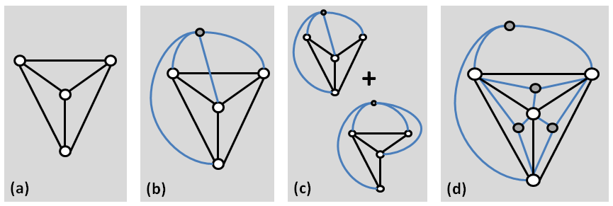
While this reduction to perfect matching provides a unique tool for energy minimization and probabilistic inference, the requirement that ${\mathcal{G}}_{1}$ be planar is a serious restriction. In particular, even if the original graph ${\mathcal{G}}$ corresponding to $E$ is planar, e.g., in the case of the grid graphs commonly used in computer vision applications, ${\mathcal{G}}_{1}$ is typically not, since the addition of edges from every node to the auxiliary node $X_{0}$ renders the graph non-planar. Assuming arbitrary values of $\theta_{i}$, those energy functions $E$ to which this method can be applied are exactly the set whose graphs ${\mathcal{G}}$ are outer-planar. An outer-planar graph is a graph with a planar embedding where all vertices share a common face (e.g., the exterior face). For such a graph, every vertex can be connected to a single auxiliary node placed inside the common face without any edges crossing so that the resulting graph ${\mathcal{G}}_{1}$ is still planar. See examples in Figure 1.

3 Inference with Dual Decomposition

Dual decomposition is a general approach for leveraging such islands of tractability in order to perform inference in more general MRFs. The application of dual decomposition to inference in graphical models was popularized by the work of Wainwright et al. (2003, 2005) on Tree-Reweighted Belief Propagation (TRW). TRW finds an optimal decomposition of an MRF into a collection of tree-structured problems where exact inference is tractable. More formally, let $t$ index a collection of subproblems defined over the same set of variables $X$ and whose parameters sum up to the original parameter values, so that $\theta=\sum_{t}\theta^{t}$. The energy function is linear in $\theta$ so we have

$$E_{MAP} =\min_{X}E(X,\Theta)=\min_{X}\sum_{t}E(X,\Theta^{t})$$ (3)

$$\qquad\geq\max_{\sum_{t}\theta^{t}=\theta}\sum_{t}\min_{X^{t}}E(X^{t},\Theta^{t})$$ (4)

The inequality arises because each subproblem $t$ is solved independently and thus may yield different solutions. On the other hand, if the solutions to the sub-problems all happen to agree then the bound is tight. The problem of maximizing the lower-bound over possible decompositions $\{\theta^{t}\}$ is convex and when inference for each sub-problem is tractable (for example, $\theta^{t}$ is tree-structured) the bound can be optimized efficiently using message passing (fixed-point iterations) based on computing min-marginals in each subproblem (Wainwright et al., 2003) or by projected subgradient methods (Komodakis et al., 2007).

A powerful tool for understanding the minimization in Equation 4 is to work with the Lagrangian dual. Equation 3 is an integer linear program over $X$, but the integrality constraints can be relaxed to a linear program over continuous parameters $\mu$ representing min-marginals which are constrained to lie within the marginal polytope, $\mu\in{\mathbb{M}}({\mathcal{G}})$. The set of constraints that define ${\mathbb{M}}({\mathcal{G}})$ are a function of the graph structure $\mathcal{G}$ and are defined by an (exponentially large) set of linear constraints that restrict $\mu$ to the set of min-marginals achievable by some consistent joint distribution (see Wainwright and Jordan, 2008). Lower-bounds of the form in Equation 4 correspond to relaxing this set of constraints to the intersection of the constraints enforced by the structure of each subproblem. For the tree-structured subproblems of TRW, this relaxation results in the so-called local polytope ${\mathbb{L}}({\mathcal{G}})$ which enforces marginalization constraints on each edge. Since ${\mathbb{L}}({\mathcal{G}})$ is an outer bound on ${\mathbb{M}}({\mathcal{G}})$, minimization yields a lower-bound on the original problem. For any relaxed set of constraints, the values of $\mu$ may not correspond to the min-marginals of any valid distribution, and so are referred to as pseudo-marginals.

One can tighten the bound in Equation 4 by adding additional subproblems to the primal (or equivalently constraints to the dual) which enforce consistency over larger sets of variables. This has been explored, e.g. by Sontag and Jaakkola (2007) who suggest adding cycle inequalities to the dual which enforce consistency of pseudo-marginals around a cycle. Since there are a large number of potential cycles present in the graph, Sontag suggests either using a cutting plane algorithm to successively add violated cycle constraints (Sontag and Jaakkola, 2007) or to only add small cycles such as triplets or quadruplets (Sontag et al., 2008) that can be enumerated with relative ease and optimized using local message passing rather than general LP solvers.

For binary problems, it is natural to consider replacing Wainwright’s tree subproblems with tractable outer-planar subgraphs. This has been explored by Globerson and Jaakkola (2007) and Batra et al. (2010) who proposed decomposing a graph into a set of planar graphs for the purposes of estimating the partition function and minimum energy state respectively. For energy minimization, it is well-known that any set of subproblems that cover every edge is sufficient to achieve the TRW bound; but what is the best set of planar graphs to use? Is it necessary to use all outer-planar or even all planar subgraphs? It turns out that the set of all outer-planar or planar subgraphs is equivalent to the set of all cycle constraints in ${\mathcal{G}}$, which can be enforced by any so-called cycle basis of the graph. This observation leads to algorithms such as reweighted perfect matching (Schraudolph, 2010), which explicitly constructs a set of subproblems that form a complete cycle basis, or incremental algorithms to enforce cycle constraints (Sontag and Jaakkola, 2007; Sontag et al., 2008; Komodakis and Paragios, 2008).

In the following sections, we focus on the case in which the original MRF is planar but the addition of the auxiliary unary node makes it non-planar. We describe a novel, compactly expressed variational approximation. We then prove that it achieves as tight a bound as decomposition into any collection of cycles or outer-planar graphs. This also gives a relatively simple proof that the tightest bounds achievable by sets of planar, outer-planar, or cycle subproblems are equivalent, and that the set of subproblems that are necessary and sufficient to achieve this bound form a cycle basis, i.e., cover every chordless cycle in the original graph at least once.

4 Planar Cycle Coverings

Figure 2: Demonstration that the minimal energy of a cycle is equal to the maximum lower-bound given by an approximation in which unary potentials are represented by a decoupled set of auxiliary variables (squares). At optimality of the variational parameters, all six cuts depicted must have equal energies and thus it is possible to choose a ground-state in which all the duplicate copies of the auxiliary node are in the same state.

Consider a planar embedding of the graph ${\mathcal{G}}$ corresponding to an MRF. Since we cannot directly connect the unary node $X_{0}$ to every node in the graph without losing planarity, we propose the following relaxation. For each face $f$ of ${\mathcal{G}}$ add an independent copy of the unary node $X_{0}^{f}$ and connect it to all vertices on the boundary of the face with weights $\theta^{f}_{i}$. Let $N_{i}$ be the set of unary node copies attached to node $i$. We split the original unary potential $\theta_{i}$ across all the unary face nodes connected to $i$ while maintaining the constraint that $\sum_{f\in N_{i}}\theta^{f}_{i}=\theta_{i}$; see Figure 1(d). Using this system we have the following relaxation

$$E_{MAP} =\min_{X:X_{0}^{f}=X_{0}}\sum_{i>j}\theta_{ij}[X_{i}\not=X_{j}]+\sum_{i,f}\theta^{f}_{i}[X_{i}\not=X^{f}_{0}]$$

$$\geq\min_{X}\sum_{i>j}\theta_{ij}[X_{i}\not=X_{j}]+\sum_{i,f}\theta^{f}_{i}[X_{i}\not=X^{f}_{0}]$$ (5)

The inequality arises because we have dropped the constraint that all copies of $X_{0}$ take on the same value. On the other hand, since the graph corresponding to the relaxation in Equation 5 is planar, we can compute the minimum exactly. Furthermore, we have freedom to adjust the $\theta^{f}_{i}$ parameters so long as they sum up to our original parameters. This yields the variational problem

$$E_{PCC}=\!\!\max_{\theta:\sum_{f}\theta^{f}_{i}=\theta_{i}}\min_{X}\sum_{i>j}\theta_{ij}[X_{i}\!\neq\!X_{j}]+\sum_{i,f}\theta^{f}_{i}[X_{i}\!\not=\!X^{f}_{0}]$$ (6)

where $E_{MAP}\geq E_{PCC}$. We refer to this construction as a planar cycle covering of the original graph since the singular potentials for each face cycle are covered by some auxiliary node (and as we shall see, all other cycles also are covered in a precise sense). Although this planar decomposition includes duplicate copies of nodes from the original problem, it differs in that there are not multiple independent subproblems but just a single, larger planar problem to be solved. This is in some ways analogous to the work of Yarkony et al. (2010) which replaces the collection of spanning trees in TRW with a single “covering tree”.

As with dual decomposition, the parameters may be optimized using subgradient or marginal fixed-point updates. For example, the subgradient updates for $\theta^{f}_{i}$ at a given setting of $X$ can be easily computed by taking a gradient and enforcing the summation constraint. This yields the update rule

$$\theta^{f}_{i}=\theta^{f}_{i}+\lambda\left([X_{i}\not=X^{f}_{0}]-\frac{1}{|N_{i}|}\sum_{g\in N_{i}}[X_{i}\not=X^{g}_{0}]\right)$$ (7)

where $|N_{i}|$ is the number of auxiliary face nodes attached to $X_{i}$ and $\lambda$ is a stepsize parameter. After each such gradient step, one must recompute the optimal setting of $X$ which can be done efficiently using perfect matching.

The subgradient update lends itself to a simple interpretation. If $X^{f}_{0}$ disagrees with $X_{i}$ but the other neighboring copies $\{X^{g}_{0}\}$ do not, then the cost for $X^{f}_{0}$ and $X_{i}$ disagreeing is increased. On the other hand, if all the copies $\{X^{g}_{0}\}$ take on the same state then the update leaves the parameters unchanged.

5 Cycle Decompositions and Cycle Covering Bounds

In this section, we show that the planar cycle cover bound $E_{PCC}$ for any planar binary MRF ${\mathcal{G}}$ is equivalent to the lower-bound given by decomposition into the collection of all cycles of ${\mathcal{G}}$.

For a given planar binary MRF with graph ${\mathcal{G}}$, consider the bound $E_{CYCLE}$ given by decomposing the MRF into the collection of all cycles of ${\mathcal{G}}$. By optimizing the allocation of parameters across these subproblems one produces a lower-bound that is generally tighter than that given by TRW and related algorithms since the subproblems can correctly account for the energy of frustrated cycles that is approximated in the tree-based bound. In fact, for planar graphs without unary potentials adding cycle subproblems is enough to make the lower-bound tight.

Lemma 5.1

The lower-bound $E_{CYCLE}$ given by the optimal cycle decomposition of a planar MRF with no unary potentials is tight.

For such an MRF the set of states corresponds exactly with the set of edge incidence vectors representing cuts in the graph. The convex hull of this set is known as the cut polytope. The connection between the cut polytope and the cycle decomposition is seen by taking the Lagrangian dual of the lower-bound optimization which yields a constrained optimization of the edge incidence vectors (pseudo-marginals) over a polytope defined by cycle inequalities. For planar graphs (or more generally graphs containing no $K_{5}$ minor), the set of cycle inequalities is sufficient to completely describe the cut polytope. See Barahona and Mahjoub (1986) for proof and related discussion by Sontag and Jaakkola (2007). Just as local edge consistency implies global consistency for a tree, cycle consistency implies global consistency for a planar binary MRF without unary potentials.

While the number of simple cycles grows exponentially in the size of the graph for general planar graphs, it is still possible to solve such a problem in polynomial time. It is not in fact necessary to include every cycle subproblem but simply a subset which form a cycle basis (Barahona, 1993). Furthermore, there exists an efficiently computable witness for identifying a violated cycle (Barahona and Mahjoub, 1986). Sontag and Jaakkola (2007) use this as the basis for a cutting plane method which successively adds cycle constraints to the dual.

We would now like to consider cycles in MRFs which do have unary potentials. We start with the simplest case of a single cycle.

Lemma 5.2

The minimum energy of a single cycle is the same as the maximum lower-bound given by the graph in which the unary potentials have been replaced by a collection of auxiliary nodes (one for each edge in the cycle) where each node in the cycle is connected to the pair of auxiliary nodes corresponding to its incident edges.

Figure 2 provides a visualization of the set of auxiliary nodes (squares) added to the cycle (circles). We refer to this as the “saw” graph. Suppose we have optimized the decomposition of unary parameters across the auxiliary node connections to maximize the lower-bound. We claim that at the optimal decomposition, there always exists a minimal energy configuration such that all the auxiliary nodes take on state $0$, making the bound equivalent to the cycle with a single auxiliary node.

Suppose we choose a minimum energy configuration of the graph but the duplicate auxiliary nodes take on mixed states. Start at some point along the cycle where there is an auxiliary node in state 0 and proceed clockwise until we find an auxiliary node in state 1. As we continue around the cycle we will encounter some later point at which the auxiliary nodes return to being in state 0. This is most easily visualized in terms of the cut separating $0$ and $1$ nodes as shown in Figure 2.

Let $X_{i}$ be the first node which is attached to a pair of disagreeing auxiliary nodes $X^{a}_{0},X^{b}_{0}$ and $X_{j}$ be the second attached to $X^{e}_{0},X^{f}_{0}$. Consider the four possible cuts highlighted in red and green in Figure 2. At the optimal decomposition of the parameters, it must be the case that these paths have equal costs. If not, then we could transfer weight (e.g. from $\theta^{a}_{i}$ to $\theta^{b}_{i}$) and increase the energy, contradicting optimality. Let $C_{1}=(\theta_{ic}+\theta^{a}_{i})=(\theta_{id}+\theta^{b}_{i})$ and $C_{2}=(\theta_{jh}+\theta^{f}_{j})=(\theta_{jg}+\theta^{e}_{j})$. If one of the four cuts shown is minimal then it must be that $C_{1}+C_{2}\leq 0$, otherwise the path which cuts none of these edges (orange) would be preferred. However, if $C_{1}+C_{2}<0$ then there is yet another cut (blue) which would achieve an energy that is lower by a non-zero amount $(C_{1}+C_{2})$ by cutting both sets of edges. Therefore, it must be the case that $C_{1}+C_{2}=0$ and thus either orange or blue cuts also represents a minimal configuration that leaves the collection of auxiliary nodes in state $0$. A similar line of argument works for the cases when $X_{c}=1$ or $X_{h}=1$ or both.

We are thus free to flip the states of the block of disagreeable auxiliary nodes and their neighbors on the cycle without changing the energy. We can then continue around the cycle in this manner until all copies of the auxiliary nodes are in state $0$ as desired. $\Box$

We are now ready to give the main result of this section.

Figure 3: Graphical depiction of Theorem 5.3 demonstrating that the planar cycle covering graph enforces constraints over all cycles of the original graph. (a) depicts the lower bound $E_{CYCLE}$ based on a decomposition into the collection of all simple cycles of the original graph. Lemma 5.2 shows that this bound is equivalent to the bound given by a corresponding collection of graphs (b) in which unary potentials are captured by multiple auxiliary nodes placed along each edge. Since every one of these graphs is a subgraph of the planar cycle covering graph (c) their minimum energy must be less than $E_{PCC}$. Finally, since the planar cycle covering graph (c) has no unary potentials, it is equal to its collection of cycles which are themselves all subgraphs of (b).

Theorem 5.3

The lower-bound given by the planar cycle covering graph is equal to the lower-bound given by decomposition into the collection of all cycles so that $E_{PCC}=E_{CYCLE}$.

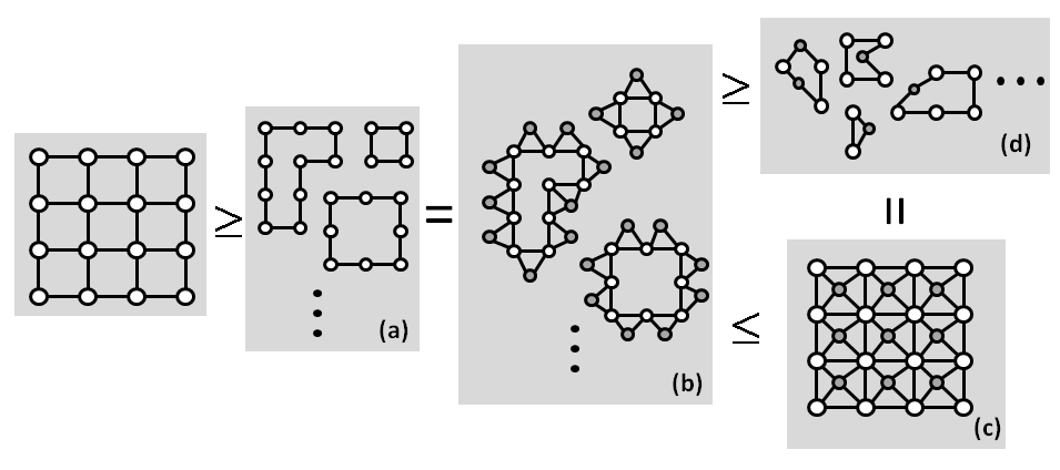
• We proceed by showing a circular sequence of inequalities. Figure 3 provides a graphical overview. Take the set of cycles which yield the bound $E_{CYCLE}$. We can apply Lemma 5.2 to transform each cycle subproblem into a corresponding “saw” containing an auxiliary node for each edge while maintaining the bound. We then observe that every such augmented cycle is a subgraph of the planar cycle covering graph. As with any such decomposition into subgraphs, the minimal energy of the cycle covering graph must be at least as large as the sum of the minimal subgraph energies and hence $E_{CYCLE}\leq E_{PCC}$. On the other hand, since the PCC graph is now a planar binary MRF with no unary terms, by Lemma 5.1 we can decompose it exactly into the collection of its constituent cycles with no loss in the bound. Finally each of these cycles is itself a subgraph of some augmented cycle and hence we must also have that $E_{CYCLE}\geq E_{PCC}$, proving equality. $\Box$

Batra et al. (2010) and Globerson and Jaakkola (2007) both propose decomposing a binary MRF into a set of tractable planar graphs. Based on the previous result, we can clearly see that the best achievable bound under such a decomposition must include a subproblem that covers every chordless cycle in the original graph. If consistency along a particular cycle is not enforced we can always arrange parameters so that the resulting bound is arbitrarily bad. We also show the converse, that outer-planar decomposition can do no better than the set of cycles.

Corollary 5.4

The best lower-bound achieved by any outer-planar decomposition for a planar MRF is no larger than $E_{PCC}$.

• Take any outer-planar decomposition of a planar MRF. We first note that an outer-planar graph may be decomposed into a forest of blocks consisting of either biconnected components or individual edges, where blocks are connected by single vertices (cut vertices). Each biconnected component in turn has a dual graph which is a tree, meaning it consists of face cycles which have one edge in common (see e.g., Syslo (1979) for a more in-depth discussion).

  We first split apart the forest into blocks. Consider any pair of blocks connected at a single cut vertex $X_{i}$. To split them, we introduce copies $X^{1}_{i}$ $X^{2}_{i}$ of the cut vertex which are allowed to take on independent states. The unary parameter $\theta_{i}$ is shared between these two copies with the constraint that $\theta^{1}_{i}+\theta^{2}_{i}=\theta_{i}$. There exists an optimal decomposition of $\theta_{i}$ which assures the two nodes share an optimizing configuration. For, suppose to the contrary that the optimal decomposition yielded a minimum energy configuration where $X^{1}_{i}$ and $X^{2}_{i}$ took on different states, say $X^{1}_{i}=0$ and $X^{2}_{i}=1$. Then, shifting weight from $\theta^{1}_{i}$ to $\theta^{2}_{i}$ would drive up the energy of such a disagreeing configuration, contradicting optimality of the decomposition.

  Once blocks have been split apart, we may apply essentially the same argument to split each biconnected component into its constituent face cycles. Consider the pair of neighboring nodes $X_{i}$,$X_{j}$ which are split into $X^{1}_{i}$,$X^{2}_{i}$,$X^{1}_{j}$, and $X^{2}_{j}$. At the optimal decomposition of the parameters $\theta_{i},\theta_{j},\theta_{ij}$, it again must be the case that the copies of the duplicated edge must share at least one optimizing configuration. If not then the parameters could be redistributed by removing weight from one or more unused states in one copy and adding it to the set of optimizing states for the other copy. This would increase the energy and thus contradict optimality of the decomposition.

  Thus any outer-planar decomposition is equivalent to a bound given by the set of constituent cycles and edges. Every one of these subproblems is a subgraph of the cycle covering graph and so the bound can be no tighter than the PCC graph bound. $\Box$

6 Experimental Results

We demonstrate the performance of the planar cycle cover bound on randomly generated Ising grid problems, and compare against two state-of-the-art approaches: max-product linear programming (MPLP) with incrementally added cycles (Sontag et al., 2008) and reweighted perfect matching (RPM) (Schraudolph, 2010).

Each problem consists a grids of size $N$x$N$ with pairwise potentials drawn from a uniform distribution $\theta_{ij}\sim U(-1,1)$. The unary potentials are generated from a uniform distribution $\theta_{i}\sim U(-a,a)$, where the magnitude $a$ determines the difficulty of the problem. Large values are relatively easy to solve, since each variable has strong local information about its optimal value; as $a$ becomes smaller the problems typically become more difficult. We generate three categories of problem, “easy” ($a=3.2$), “medium” ($a=0.8$), and “hard” ($a=0.2$), and show the results on each class of problem separately. To make it easy to test convergence, we scaled the weights by $500$ and rounded them to integers. Thus a gap of less than $1$ between lower and upper bounds provides a certificate of optimality.

We implemented the PCC bound using the Blossom V implementation of Kolmogorov and Zabih (2004). At each step $t$ we obtain both a lower-bound $E_{PCC}^{t}$ and a configuration of $X=[X_{1},\ldots,X_{N}]$ and the copies $\{X_{0}^{f}\}$. We compute the energy of two possible joint solutions, $X$ and its complement $\bar{X}$, and save the best solution found so far and its energy $\hat{E}^{t}$ as a current upper bound. The variational parameters are updated using the projected sub-gradient given in Equation 7, and the step size $\lambda$ is chosen using Polyak’s step size rule, i.e., given sub-gradient $g(\theta)$ we choose $\lambda=\frac{1}{2}(\hat{E}^{t}-E_{PCC}^{t})/\|g\|^{2}$. The incremental update feature of Blossom V is used to speed up successive optimizations as the variational parameters are modified.

For both MPLP and RPM, we used the original authors’ code available online. MPLP first runs an optimization corresponding to the tree-reweighted lower bound (TRW), then successively tightens this bound by trying to identify cycles whose constraints are significantly violated and adding those subproblems to the collection. For grids, it enumerates and checks each square of four variables; we modified the code slightly to ensure that any given square is added only once. Because weak tree agreement can lead to suboptimal fixed points in MPLP, we tried both the standard message updates and a version which used subgradient steps, but found little difference and report only the fixed point update results. We also note that because this implementation of MPLP explicitly enumerates only a subset of cycles, the MPLP implementation may not provide the tightest possible lower-bound, an effect we observe in our experiments.

For RPM, we used the author’s implementation IsInf, which uses a bundle-trust optimization subroutine for its subgradient updates. IsInf does not compute upper bounds (proposed solutions) frequently; in plots showing the change in bounds over time we modified the code to also return such a solution, but used the default behavior for our timing comparisons.

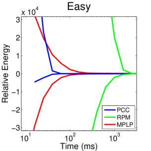
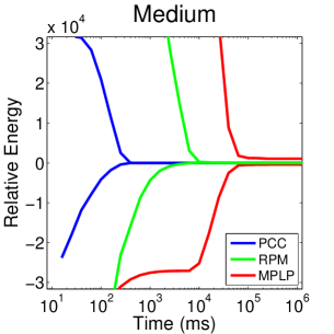
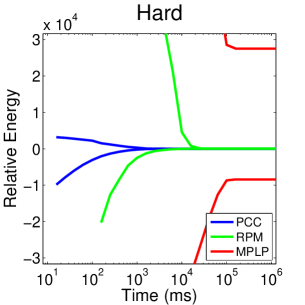
Figure 4 shows the upper and lower bounds found by each algorithm as a function of time, for a single $32\times 32$ problem instance from each of the three categories. For the “easy” problem, all three methods find and verify the optimal solution (zero duality gap); in this case, MPLP converges more quickly than RPM, and PCC is faster still. For the “medium” problem, we see that MPLP converges more slowly and to a small duality gap, with RPM slightly faster and PCC still fastest. For the “hard” problem, MPLP has a large duality gap; in this case RPM and PCC still converge to and verify the optimum. In all cases, PCC is significantly faster than the other methods.

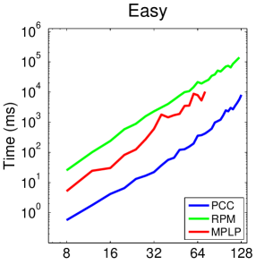
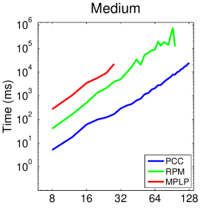
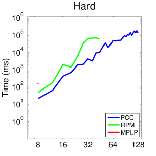
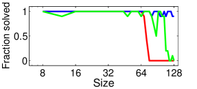
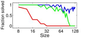
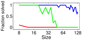
Figure 5 shows timing results as a function of problem size for all three algorithms. Since each method may converge (return a provably optimal solution) on some problems but not others, we report two quantities: the geometric mean of the time over all problems for which the method converged (upper row), and the fraction of problems that the method successfully solved (lower row). As can be seen, PCC is significantly faster than the other two methods across both problem difficulty and size, and successfully solves a greater percentage of the problems.

Figure 4: Average convergence behavior of lower- and upper-bounds for randomly generated 32x32 Ising grid problems. We compare PCC, the planar cycle cover bound (blue) to RPM (green) and MPLP (red) for easy, medium and hard problems. The problem difficulty is controlled by the relative influence of unary and pairwise potentials. Energies are averaged over 10 random problem instances and plotted relative to a MAP energy of $0$.

Figure 5: Convergence times as a function of problem size for randomly generated Ising grid problems. We compare PCC (blue) to RPM (green) and MPLP (red) for easy, medium and hard problems. We record times for upper- and lower- bounds to converge averaged over 10 problem instances. We only include in the average convergence time those problem instances for which an algorithm was able to find the MAP configuration (a duality gap of less than 1). The second row of plots shows in each case the fraction of problems for which this happened.

7 Discussion

We have described a new variational bound for performing inference in planar binary MRFs. Our bound subsumes those given by both the tree-reweighted (TRW) and outer-planar decompositions of such a graph since it implicitly includes every edge and cycle as a sub-problem. Unlike approaches such as MPLP which successively add cycles, we are able to get the full benefit of all cycle constraints immediately. As a result we achieve fast convergence in practice.

The PCC graph bound is limited to planar binary problems. We are currently exploring routes to remove these limitations. For example, in general non-planar graphs, we can triangulate the graph to get a cycle basis of triangles and then “glue” those triangles together into the smallest possible planar graph. In addition to MAP inference, it will also be interesting to see how the PCC graph relates to variational approximations to the marginals.

Acknowledgements

This work was supported by a grant from the UC Labs Research Program

References

- Barahona (1982) F. Barahona. On the computational complexity of Ising spin glass models. Journal of Physics A: Mathematical, Nuclear and General, 15(10):3241-3253, 1982.
- Barahona (1993) F. Barahona. On cuts and matchings in planar graphs. Mathematical Programming, 60:53–68, 1993.
- Barahona and Mahjoub (1986) F. Barahona and A. Mahjoub. On the cut polytope. Mathematcial Programming, 36:157–173, 1986.
- Batra et al. (2010) D. Batra, A. Gallagher, D. Parikh, and T. Chen. Beyond trees: MRF inference via outer-planar decomposition. In CVPR, 2010.
- Edmonds (1965) J. Edmonds. Paths, trees, and flowers. Canad. J. Math., 17:449–467, 1965.
- Fisher (1961) M. Fisher. Statistical mechanics of dimers on a plane lattice. Physical Review, 124 (6):1664-1672, 1961.
- Fisher (1966) M. Fisher. On the dimer solution of planar Ising models. 7(10):1776-1781, 1966.
- Globerson and Jaakkola (2007) A. Globerson and T. Jaakkola. Approximate inference using planar graph decomposition. In NIPS, pages 473–480, 2007.
- Kappes et al. (2010) J. Kappes, S. Schmidt, and C. Schnoerr. MRF inference by k-fan decomposition and tight lagrangian relaxation. In ECCV, 2010.
- Kasteleyn (1961) P. Kasteleyn. The statistics of dimers on a lattice: I. the number of dimer arrangements on a quadratic lattice. Physica, 27(12):1209-1225, 1961.
- Kasteleyn (1967) P. Kasteleyn. Graph theory and crystal physics. In Frank Harary, editor, Graph Theory and Theoretical Physics, pages 43–110, 1967.
- Kolmogorov (2006) V. Kolmogorov. Convergent tree-reweighted message passing for energy minimization. IEEE Trans. Pattern Anal. Machine Intell., 28(10):1568–1583, 2006.
- Kolmogorov (2009) V. Kolmogorov. Blossom V: A new implementation of a minimum cost perfect matching algorithm. Mathematical Programming Computation, 1(1):43–67, 2009.
- Kolmogorov and Zabih (2004) V. Kolmogorov and R. Zabih. What energy functions can be minimized via graph cuts? IEEE Trans. Pattern Anal. Machine Intell., 26(2):147–159, 2004.
- Komodakis and Paragios (2008) N. Komodakis and N. Paragios. Beyond loose LP-relaxations: Optimizing MRFs by repairing cycles. In ECCV, 2008.
- Komodakis et al. (2007) N. Komodakis, N. Paragios, and G. Tziritas. MRF optimization via dual decomposition: Message-passing revisited. In ICCV, Rio de Janeiro, Brazil, Oct. 2007. doi: 10.1109/ICCV.2007.4408890.
- Schraudolph (2010) N. Schraudolph. Polynomial-time exact inference in np-hard binary MRFs via reweighted perfect matching. In AISTATS, 2010.
- Schraudolph and Kamenetsky (2008) N. Schraudolph and D. Kamenetsky. Efficient exact inference in planar Ising models. Technical Report 0810.4401, Oct. 2008.
- Shih et al. (1990) W.-K. Shih, S. Wu, and Y. Kuo. Unifying maximum cut and minimum cut of a planar graph. IEEE Transactions on Computers, 39:694–697, 1990.
- Sontag and Jaakkola (2007) D. Sontag and T. Jaakkola. New outer bounds on the marginal polytope. In NIPS, 2007.
- Sontag et al. (2008) D. Sontag, T. Meltzer, A. Globerson, Y. Weiss, and T. Jaakkola. Tightening LP relaxations for MAP using message passing. In UAI, 2008.
- Syslo (1979) M. Syslo. Characterizations of outerplanar graphs. Discrete Mathematics, 26:1, 47-53, 1979.
- Torresani et al. (2008) L. Torresani, V. Kolmogorov, and C. Rother. Feature correspondence via graph matching: Models and global optimization. In ECCV, pages 596–609, 2008.
- Wainwright and Jordan (2008) M. J. Wainwright and M. I. Jordan. Graphical models, exponential families, and variational inference. Foundations and Trends in Machine Learning, 1:1–305, 2008.
- Wainwright et al. (2003) M. J. Wainwright, T. Jaakkola, and A. S. Willsky. Tree–based reparameterization analysis of sum–product and its generalizations. IEEE Trans. Inform. Theory, 49(5):1120–1146, May 2003.
- Wainwright et al. (2005) M. J. Wainwright, T. Jaakkola, and A. S. Willsky. MAP estimation via agreement on (hyper)trees: message-passing and linear programming approaches. IEEE Trans. Inform. Theory, 51(11):3697–3717, 2005.
- Yarkony et al. (2010) J. Yarkony, C. Fowlkes, and A. Ihler. Covering trees and lower-bounds on the quadratic assignment. In CVPR, 2010.