The Narrow Escape problem in a flat cylindrical microdomain with application to diffusion in the synaptic cleft

Abstract

The mean first passage time (MFPT) for a Brownian particle to reach a small target in cellular microdomains is a key parameter for chemical activation. Although asymptotic estimations of the MFPT are available for various geometries, these formula cannot be applied to degenerated structures where one dimension of is much smaller compared to the others. Here we study the narrow escape time (NET) problem for a Brownian particle to reach a small target located on the surface of a flat cylinder, where the cylinder height is comparable to the target size, and much smaller than the cylinder radius. When the cylinder is sealed, we estimate the MFPT for a Brownian particle to hit a small disk located centrally on the lower surface. For a laterally open cylinder, we estimate the conditional probability and the conditional MFPT to reach the small disk before exiting through the lateral opening. We apply our results to diffusion in the narrow synaptic cleft, and compute the fraction and the mean time for neurotransmitters to find their specific receptors located on the postsynaptic terminal. Finally, we confirm our formulas with Brownian simulations.

1 Introduction

The problem of computing the mean first passage time (MFPT) for a Brownian particle to reach a small target located on a surface of a microdomain, also referred to as the Narrow Escape Time (NET) [36, 14], is ubiquitous in biophysics and cellular biology because it corresponds to determining the forward binding rate of chemical reactions [39, 2, 38, 10]. Applications of the NET ranges from quantitative analysis for the resident time of receptors in the postsynaptic density [14, 27, 35, 12], a fundamental microdomain associated to synaptic transmission and plasticity [8], to scaling laws in physics [7], early steps of viral infection [11, 19, 18], or the hydrolysis rate of activated phosphodiesterase in rod photoreceptors [23, 24].

Recent analytical approaches lead to asymptotic formula for the NET in a confined geometry [36, 37, 30, 29]. For example, in a three dimensional domain of volume $V$ with isoperimetric ratio of order 1, and with no bottlenecks, the overall NET to an absorbing circular hole of (dimensionless) radius $a$ centered at $\mbox{\boldmath$x$}_{s}$ on the surface is [30]

$$\tau=\frac{|V|}{4aD}\left(1+\frac{L(\mbox{\boldmath$x$}_{s})+N(\mbox{\boldmath$x$}_{s})}{2\pi}a\ln a+O(a\ln a))\right)^{-1}\,,$$ (1)

where $D$ is the diffusion constant, $L(\mbox{\boldmath$x$}_{s})$ and $N(\mbox{\boldmath$x$}_{s})$ are the principal curvatures at $x_{s}$. In the case of a sphere, a precise asymptotic expression with the first three terms was recently obtained in [6], where the $O(1)$ term depends on the regular part of the Green’s function. The NET computations were further generalized to the case of several holes [15, 21, 6], and to stochastic dynamics with a potential well [28, 35].

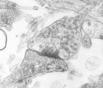
However, the NET formula (1) cannot be directly applied to degenerated microdomains where one dimension is much smaller than the others. This is for example the case for the synaptic cleft separating pre- and post-synaptic neuronal terminals (Fig. 1a), which can be approximated as a flat cylinder with height much smaller compared to its width [3]. Furthermore, in retinal rod photoreceptors sustaining night vision, the outer segment contains thousands of piled flat cylinders that define the photoresponse and the fidelity of the vision under dim light conditions [25, 13, 23].

The goal of this paper is to extend the NET analysis to degenerate domains. More specifically, we study the NET of a Brownian particle in a flat cylinder, where the cylinder height $h$ is much smaller compared to the cylinder radius $R$ ($h\ll R$), with a small circular hole of radius $a$ centered on the bottom cylinder surface (Fig. 1b). In the first part, we will analyze the NET to exit the cylindrical domain when the boundary is reflecting everywhere except at the small hole, where it is absorbing. Due to the radial symmetry, the solution of the the mixed boundary value problem can be expanded in terms of Bessel functions. For a flat cylinder with $h\ll R$ and $R\gg a$, we find that the NET is given by

$$\tau\approx\frac{|V|}{aD}\frac{a_{0}\left(\frac{h}{a}\right)}{\sqrt{2}}+\frac{R^{2}}{8D}\left(4\ln\left(\frac{R}{a}\right)-3\right)\,,$$ (2)

where the function ${a_{0}\left(\frac{h}{a}\right)}/{\sqrt{2}}\in[0.07,0.25]$ is depicted in Fig. 2a. Although we derive (2) for $h\ll R$, we expect that it remains a valid approximation until $h\sim R$, in which case $a_{0}(\frac{h}{a})\sim\frac{1}{4}$ and the leading order terms in (2) and (1) coincide. We note that the log-contribution in (1) comes from the local property of the boundary at the hole, whereas in (2) it originates from the degenerated geometry.

In the second part of the paper, we study a cylinder that is open at lateral boundary, and we present asymptotic estimates for the conditional probability $p$ and the conditional mean time $\tau_{c}$ that a Brownian particle reaches the small hole before leaving the domain through the lateral boundary. For example, for a flat cylinder with $h\sim a$ and $R\gg a$, when the particle starts at the upper boundary at position $(r=0,z=h)$ opposite to the small hole, the conditional probability $p(0,h)$ and the conditional mean time $\tau_{c}(0,h)$ are ((95), (129) and (163))

$$\begin{array}[]{rcl}\displaystyle\tau(0,h)&\approx&\displaystyle{\frac{|V|}{aD}\frac{a_{0}(h/a)}{I_{0}(\frac{\pi a}{2h})}},\\ \\ \displaystyle{p(0,h)}&\approx&\displaystyle{1-\frac{2D}{R^{2}\ln(R/a)}\tau(0,h)},\\ \\ \displaystyle\tau_{c}(0,h)&\approx&\displaystyle{\frac{\displaystyle{1-\frac{\sqrt{2}D}{R^{2}\ln(R/a)}}\displaystyle{I_{0}(\frac{\pi a}{2h})}\tau(0,h)}{\displaystyle{1-\ \frac{2D}{R^{2}\ln(R/a)}\tau(0,h)}}}\displaystyle{\frac{\tau(0,h)}{2(\ln(R/a))^{2}}},\end{array}$$ (8)

where $\alpha=R/a\gg 1$, $\beta=h/a\sim 1$ and $\tau(0,h)$ is the mean time to reach the small hole when the cylinder is closed. These asymptotic expressions can be applied to study diffusion in the synaptic cleft, where synaptic transmission depends on neurotransmitters that are released at the presynaptic terminal from vesicles and activate receptors located on the opposite post-synaptic neuron (Fig. 1). The transmission efficiency depends crucially on the conditional probability for a diffusing neurotransmitter to hit a functional receptor before leaving the synaptic cleft.

2 Mean time to find a small target in a bounded cylindrical compartment

We shall now present our analysis to estimate the MFPT $\tau(\mbox{\boldmath$x$})$ for a Brownian molecule, initially located at position $\mbox{\boldmath$x$}=(x_{1},x_{2},z)$, to escape a cylinder of radius $R$ and height $h$ (Fig.1) through a small circular hole of radius $a$ located centrally on the lower surface at $z=0$. The cylindrical surface is reflecting, except for the small hole where it is absorbing. Due to the radial symmetry, the MFPT is a function of the radius $r=\sqrt{x_{1}^{2}+x_{2}^{2}}$ and the height $z$. Using the small hole radius $a$, we define the dimensionless parameters and variables

$$x=\frac{r}{a}\,,\quad y=\frac{z}{a}\,,\quad\alpha=\frac{R}{a}\,,\quad\beta=\frac{h}{a}\,,\quad|\Omega|=\frac{|V|}{a^{3}}=\pi\beta\alpha^{2}\,,$$

and the scaled MFPT

$$\hat{\tau}(x,y)=\frac{aD}{|V|}\tau(r,z)=\frac{D}{\pi R^{2}\beta}\tau(r,z)\,,$$ (9)

which is a solution of [26]

$$\begin{array}[]{rcl}\displaystyle\left(\frac{1}{x}\frac{\partial}{\partial x}x\frac{\partial}{\partial x}+\frac{\partial^{2}}{\partial y^{2}}\right)\hat{\tau}(x,y)&=&\displaystyle-\frac{1}{|\Omega|}\,,\quad x\in\Omega\\ \displaystyle\hat{\tau}(x,y)&=&0\,,\quad y=0\,,\,x<1\\ \displaystyle\frac{\partial}{\partial y}\hat{\tau}(x,y)&=&0\,,\quad y=0\,,\,1<x<\alpha\\ \displaystyle\frac{\partial}{\partial y}\hat{\tau}(x,y)\Big{|}_{y=\beta}=0\,,&&\displaystyle\frac{\partial}{\partial x}\hat{\tau}(x,y)\Big{|}_{x=\alpha}=0\,.\end{array}$$ (14)

Our goal is to obtain a solution for (14) and to clarify its dependency on the parameters $\alpha$ and $\beta$. To study the shape of the boundary layer, we note that (14) corresponds to a heat equation where the total amount of heat produced in $\Omega$ is one, independent of $\alpha$ and $\beta$. Furthermore, because the scaled radius of the hole through which the heat dissipates is one, it follows that $\hat{\tau}(x,y)$ has a finite asymptotic limit in the neighborhood of the hole for $\alpha\to\infty$ and $\beta\to\infty$.

Figure 1: (a) EM picture of a synapse showing a synaptic cleft and the two pre and post-synaptic terminals. (b) Schematic representation of a Brownian trajectory in a cylinder of height $h$ and radius $R$ with reflecting boundaries, except at the small absorbing disk of radius $a\ll R$, located centrally on the lower surface. We are interested in the case of a flat cylinder with $R\gg a$ and $h\sim a$.

2.1 Equation for the scaled MFPT $\hat{\tau}(x,y)$

To derive the solution $\hat{\tau}(x,y)$ of (14), we consider the two domains

$$\Omega_{i}=\{x|x<1\}\hbox{ and }\Omega_{o}=\{x|1<x<\alpha\},$$

and obtain for $\hat{\tau}(x,y)$ the representation

$$\hat{\tau}(x,y)=\left\{\begin{array}[]{l}\displaystyle\hat{\tau}_{i}(x,y)\,,\quad(x,y)\in\Omega_{i}\\ \\ \displaystyle\hat{\tau}_{o}(x,y)\,,\quad(x,y)\in\Omega_{o}\,.\end{array}\right.$$ (18)

To ensure that $\hat{\tau}(x,y)$ is a solution of (14) in $\Omega$, $\hat{\tau}(x,y)$ and the flux $\frac{\partial}{\partial x}\hat{\tau}(x,y)$ have to be continuous at $x=1$, leading to the conditions

$$\begin{array}[]{lll}\displaystyle\hat{\tau}_{i}(1,y)&=&\displaystyle\hat{\tau}_{o}(1,y)\,,\quad 0<y<\beta\\ \\ \displaystyle\frac{\partial\hat{\tau}_{i}(x,y)}{\partial x}\Big{|}_{x=1}&=&\displaystyle\frac{\partial\hat{\tau}_{o}(x,y)}{\partial x}\Big{|}_{x=1}\,,\quad 0<y<\beta\,.\end{array}$$ (22)

Using a separation of variable method, we expand $\tau_{i}(x,y)$ and $\tau_{o}(x,y)$ in series

$$\tau_{i}(x,y) = \sum_{n=0}^{\infty}b_{n}q_{n}(x)v_{n}(y)+w_{i}(x,y)$$ (23)

$$\tau_{o}(x,y) = \sum_{n=0}^{\infty}a_{n}p_{n}(x)u_{n}(y)+w_{o}(x,y)$$ (24)

where

$$\begin{array}[]{c}\displaystyle k_{n}=\frac{n\pi}{\beta}\,,\quad l_{n}=\frac{(n+\frac{1}{2})\pi}{\beta}\,,\\ \displaystyle u_{0}=\frac{1}{\sqrt{2}}\,,\quad u_{n}(y)=\cos\left(k_{n}y\right)\quad(n\geq 1)\,,\quad v_{n}(y)=\sin(l_{n}y)\quad(n\geq 0)\,,\end{array}$$ (27)

$w_{i}(x,y)$ and $w_{o}(x,y)$ are the inhomogeneous solutions of (14) that vanish at $x=1$, and $p_{n}(x)$ and $q_{n}(x)$ will be derived below in terms of the modified Bessel functions $I_{0}(x)$ and $K_{0}(x)$, and are normalized such that $p_{n}(1)=q_{n}(1)=1$.

The functions $v_{n}(y)$ and $u_{n}(y)$ satisfy the orthogonality relations

$$\begin{array}[]{c}\displaystyle\int_{0}^{\beta}u_{n}(y)u_{m}(y)dy=\int_{0}^{\beta}v_{n}(y)v_{m}(y)dy=\frac{\beta}{2}\delta_{nm}\\ \displaystyle\int_{0}^{\beta}v_{n}(y)u_{m}(y)dy=\frac{\beta}{2}\xi_{nm}\,,\end{array}$$ (30)

where

$$\xi_{nm}=\left\{\begin{array}[]{l}\displaystyle\frac{2}{\beta}\frac{l_{n}}{l_{n}^{2}-k_{m}^{2}}=\frac{2}{\pi}\frac{(n+\frac{1}{2})}{(n+\frac{1}{2})^{2}-m^{2}}\,,\quad m\geq 1\\ \\ \displaystyle\frac{\sqrt{2}}{\beta l_{n}}=\frac{\sqrt{2}}{\pi}\frac{1}{n+\frac{1}{2}}\,,\quad m=0\end{array}\right.$$ (34)

is an orthogonal matrix satisfying

$$\sum_{p=0}^{\infty}\xi_{pn}\xi_{pm}=\sum_{p=0}^{\infty}\xi_{np}\xi_{mp}=\delta_{nm}\,.$$

Using the orthogonality relations, we obtain the expansions

$$u_{n}(y)=\sum_{m=0}^{\infty}\xi_{mn}v_{m}(y)\,,\quad v_{n}(y)=\sum_{m=0}^{\infty}\xi_{nm}u_{m}(y)\,.$$ (35)

2.1.1 Derivation of $p_{n}(x)$ and $w_{o}(x,y)$

The equation for $\hat{\tau}_{o}(x,y)$ in $\Omega_{o}$ is

$$\begin{array}[]{c}\displaystyle\left(\frac{1}{x}\frac{\partial}{\partial x}x\frac{\partial}{\partial x}+\frac{\partial^{2}}{\partial y^{2}}\right)\hat{\tau}_{o}(x,y)=-\frac{1}{|\Omega|}\,,\quad(x,y)\in\Omega_{o}\\ \displaystyle\frac{\partial}{\partial y}\hat{\tau}_{o}(x,y)\Big{|}_{y=0,\beta}=0\,,\quad\frac{\partial}{\partial x}\hat{\tau}_{o}(x,y)\Big{|}_{x=\alpha}=0\end{array}$$ (38)

and we choose $w_{o}(x,y)$ to satisfy

$$\begin{array}[]{c}\displaystyle\left(\frac{1}{x}\frac{\partial}{\partial x}x\frac{\partial}{\partial x}+\frac{\partial^{2}}{\partial y^{2}}\right)w_{o}(x,y)=-\frac{1}{|\Omega|}\,,\quad(x,y)\in\Omega_{o}\\ \displaystyle w_{o}(1,y)=0\,,\quad\frac{\partial}{\partial y}w_{o}(x,y)\Big{|}_{y=0,\beta}=0\,,\quad\frac{\partial}{\partial x}w_{o}(x,y)\Big{|}_{x=\alpha}=0.\end{array}$$ (40)

The solution for $w_{o}(x,y)$ is

$$w_{o}(x,y)=\frac{\ln x}{2\pi\beta}-\frac{x^{2}-1}{4|\Omega|}\,.$$ (41)

Inserting $\hat{\tau}_{o}(x,y)$ from (24) into (38) yields for $p_{n}(x)$ the equations

$$\begin{array}[]{c}\displaystyle\left(\frac{1}{x}\frac{\partial}{\partial x}x\frac{\partial}{\partial x}-k_{n}^{2}\right)p_{n}(x)=0\,,\quad 1<x<\alpha\\ \displaystyle p_{n}(1)=1\,,\quad\frac{\partial}{\partial x}p_{n}(x)\Big{|}_{x=\alpha}=0\,.\end{array}$$ (43)

Using the modified Bessel functions $I_{0}(x)$ and $K_{0}(x)$ and the relations [5] ($I_{0}^{\prime}(x)=I_{1}(x)$, $K_{0}^{\prime}(x)=-K_{1}(x)$, we obtain

$$p_{n}(x)=\frac{F_{0}(k_{n}x,k_{n}\alpha)}{F_{0}(k_{n},k_{n}\alpha)}\,,$$ (44)

with

$$F_{0}(x,y)=I_{0}(x)K_{1}(y)+K_{0}(x)I_{1}(y)\,.$$

2.1.2 Derivation of $q_{n}(x)$ and $w_{i}(x,y)$

Proceeding similarly to the previous paragraph, the equation for $\hat{\tau}_{i}(x,y)$ in $\Omega_{i}$ is

$$\begin{array}[]{c}\displaystyle\left(\frac{1}{x}\frac{\partial}{\partial x}x\frac{\partial}{\partial x}+\frac{\partial^{2}}{\partial y^{2}}\right)\hat{\tau}_{i}(x,y)=-\frac{1}{|\Omega|}\,,\quad(x,y)\in\Omega_{i}\\ \displaystyle\hat{\tau}_{i}(x,0)=0\,,\quad\frac{\partial}{\partial y}\hat{\tau}_{i}(x,y)\Big{|}_{y=\beta}=0\,.\end{array}$$ (47)

We choose $w_{i}(x,y)$ to satisfy

$$\begin{array}[]{c}\displaystyle\left(\frac{1}{x}\frac{\partial}{\partial x}x\frac{\partial}{\partial x}+\frac{\partial^{2}}{\partial y^{2}}\right)w_{i}(x,y)=-\frac{1}{|\Omega|}\,,\quad(x,y)\in\Omega_{i}\\ \displaystyle w_{i}(1,y)=0\,,\quad w_{i}(x,0)=0\,,\quad\frac{\partial}{\partial y}w_{i}(x,y)\Big{|}_{y=\beta}=0\,,\end{array}$$ (49)

with solution

$$\begin{array}[]{lll}\displaystyle w_{i}(x,y)&=&\displaystyle\frac{1}{|\Omega|}\sum_{n=1}^{\infty}c_{n}J_{0}(z_{n}x)\frac{\cosh(z_{n}(\beta-y))}{\cosh(z_{n}\beta)}-\frac{x^{2}-1}{4|\Omega|}\\ \displaystyle&=&\displaystyle\frac{1}{|\Omega|}\sum_{n=1}^{\infty}c_{n}J_{0}(z_{n}x)\left(\frac{\cosh(z_{n}(\beta-y))}{\cosh(z_{n}\beta)}-1\right)\,,\end{array}$$ (52)

where $z_{n}$ are the positive zeros of the Bessel function $J_{0}(x)$, and the coefficients $c_{n}$ are given by

$$c_{n}=\frac{2}{J_{0}^{\prime}(z_{n})^{2}}\int_{0}^{1}J_{0}(z_{n}x)\frac{x^{2}-1}{4}xdx\,.$$ (53)

To derive expression (53), we used the orthogonality relation [5]

$$\int_{0}^{1}J_{0}(z_{n}x)J_{0}(z_{m}x)xdx=\delta_{nm}\frac{1}{2}\left(J_{0}(z_{n})^{2}+J_{0}^{\prime}(z_{n})^{2}\right).$$

Inserting $\hat{\tau}_{i}(x,y)$ from (23) into (47) gives for $q_{n}(x)$ the equation

$$\begin{array}[]{c}\displaystyle\left(\frac{1}{x}\frac{\partial}{\partial x}x\frac{\partial}{\partial x}-l_{n}^{2}\right)q_{n}(x)=0\,,\quad x<1\\ \displaystyle q_{n}(1)=1\,,\end{array}$$ (55)

and the solution that is regular at $x=0$ is

$$q_{n}(x)=\frac{I_{0}(l_{n}x)}{I_{0}(l_{n})}\,.$$ (56)

2.1.3 General expression for $\hat{\tau}(x,y)$

Using the expressions for $p_{n}(x)$, $q_{n}(x)$, $w_{i}(x,y)$ and $w_{o}(x,y)$, the NET solution is

$$\hat{\tau}(x,y)=\left\{\begin{array}[]{l}\displaystyle\hat{\tau}_{i}(x,y)=\sum_{n=0}^{\infty}b_{n}\frac{I_{0}(l_{n}x)}{I_{0}(l_{n})}v_{n}(y)+w_{i}(x,y)\,,\quad x\leq 1\\ \\ \displaystyle\hat{\tau}_{o}(x,y)=\sum_{n=0}^{\infty}a_{n}\frac{F_{0}(k_{n}x,k_{n}\alpha)}{F_{0}(k_{n},k_{n}\alpha)}u_{n}(y)+\frac{\ln x}{2\pi\beta}-\frac{x^{2}-1}{4|\Omega|}\,,\quad 1\leq x\leq\alpha,\end{array}\right.$$ (60)

where the unknown coefficients $a_{n}$ and $b_{n}$ will be determined by patching the two expressions at $x=1$. The continuity condition for $\hat{\tau}(x,y)$ at $x=1$ gives

$$\sum_{n=0}^{\infty}a_{n}u_{n}(y)=\sum_{n=0}^{\infty}b_{n}v_{n}(y)\,,$$

and using the expansions in (35), we obtain that $a_{n}$ and $b_{n}$ are related by

$$b_{n}=\sum_{m=0}^{\infty}\xi_{nm}a_{m}\,,\quad a_{m}=\sum_{n=0}^{\infty}\xi_{nm}b_{n}\,.$$ (61)

The continuity condition for the flux at $x=1$ gives

$$\sum_{n=0}^{\infty}b_{n}l_{n}\frac{I_{1}(l_{n})}{I_{0}(l_{n})}v_{n}(y)-\sum_{n=1}^{\infty}a_{n}k_{n}\frac{F_{1}(k_{n},k_{n}\alpha)}{F_{0}(k_{n},k_{n}\alpha)}u_{n}(y)=\frac{1}{2\pi\beta}-\frac{1}{2|\Omega|}-\frac{\partial}{\partial x}w_{i}(x,y)\Big{|}_{x=1}\,,$$

with

$$F_{1}(x,y)=\frac{\partial}{\partial x}F_{0}(x,y)=I_{1}(x)K_{1}(y)-K_{1}(x)I_{1}(y)\,.$$

This can be rewritten as

$$\sum_{n=0}^{\infty}b_{n}\beta_{n}v_{n}(y)+\sum_{n=0}^{\infty}a_{n}\alpha_{n}u_{n}(y)=\sum_{n=0}^{\infty}\gamma_{n}u_{n}(y)\,.$$ (62)

where

$$\begin{array}[]{c}\displaystyle\alpha_{0}=0\,,\quad\alpha_{n}=-k_{n}\frac{F_{1}(k_{n},k_{n}\alpha)}{F_{0}(k_{n},k_{n}\alpha)}\,\,(n\geq 1)\,,\quad\displaystyle\beta_{n}=l_{n}\frac{I_{1}(l_{n})}{I_{0}(l_{n})}\end{array}$$ (64)

and the $\gamma_{n}$ are implicitly defined by the equation

$$\sum_{n=0}^{\infty}\gamma_{n}u_{n}(y)=\frac{1}{2\pi\beta}-\frac{1}{2|\Omega|}-\frac{\partial}{\partial x}w_{i}(x,y)\Big{|}_{x=1}\,.$$ (65)

By using the expansions in (35) we obtain from (62)

$$\begin{array}[]{lll}\displaystyle\sum_{m=0}^{\infty}\alpha_{m}\xi_{nm}a_{m}+\beta_{n}b_{n}&=&\displaystyle\sum_{m=0}^{\infty}\xi_{nm}\gamma_{m}\\ \displaystyle\alpha_{n}a_{n}+\sum_{m=0}^{\infty}\beta_{m}b_{m}\xi_{mn}&=&\displaystyle\gamma_{n}\,.\end{array}$$ (68)

Finally, using the relations between $a_{n}$ and $b_{n}$ given in (61), we obtain the matrix equations

$$\begin{array}[]{lll}\displaystyle\sum_{m=0}^{\infty}(\beta_{n}+\alpha_{m})\xi_{nm}a_{m}&=&\displaystyle\sum_{m=0}^{\infty}\xi_{nm}\gamma_{m}\\ \displaystyle\sum_{m=0}^{\infty}(\beta_{m}+\alpha_{n})\xi_{mn}b_{m}&=&\displaystyle\gamma_{n}\,.\end{array}$$ (71)

For given $\alpha$ and $\beta$, by truncating and numerically solving these equations we find approximated values for $a_{n}$ and $b_{n}$, and from this we obtain an approximation for $\hat{\tau}(x,y)$. We will analyze the equations for $a_{n}$ and $b_{n}$ in more detail later on.

2.2 MFPT with a uniform initial distribution

We shall first consider the average MFPT $\hat{\tau}(x)$ when the Brownian particle is initially uniformly distributed at radial position $x$. Using (60) we obtain

$$\hat{\tau}(x)=\frac{1}{\beta}\int_{0}^{\beta}\hat{\tau}(x,y)dy=\left\{\begin{array}[]{l}\displaystyle\hat{\tau}_{i}(x)=\frac{1}{\beta}\sum_{n=0}^{\infty}\frac{b_{n}}{l_{n}}\frac{I_{0}(l_{n}x)}{I_{0}(l_{n})}+\frac{1}{\beta}\int_{0}^{\beta}w_{i}(x,y)dy\,,\quad x\in\Omega_{i}\\ \\ \displaystyle\hat{\tau}_{o}(x)=\frac{a_{0}}{\sqrt{2}}+\frac{\ln x}{2\pi\beta}-\frac{x^{2}-1}{4|\Omega|}\,,\quad x\in\Omega_{o}.\end{array}\right.$$ (75)

Expression (75) shows that $\frac{a_{0}}{\sqrt{2}}$ is the averaged MFPT for Brownian particles that are initially uniformly distributed at $x=1$. The expression for $\hat{\tau}_{o}(x)$ has an intuitive interpretation: the escape time starting at $x\geq 1$ is the sum of the average time to reach $x=1$, plus the escape time starting at $x=1$.

The average MFPT $\hat{\tau}$ for particles that are initially uniformly distributed in $\Omega$ is

$$\hat{\tau} = \frac{1}{|\Omega|}\int_{\Omega}\hat{\tau}(x,y)dV=\frac{|\Omega_{i}|}{|\Omega|}\frac{1}{|\Omega_{i}|}\int_{\Omega_{i}}\hat{\tau}(x,y)dV+\frac{|\Omega_{o}|}{|\Omega|}\frac{1}{|\Omega_{o}|}\int_{\Omega_{o}}\hat{\tau}(x,y)dV$$ (76)

$$= \frac{|\Omega_{i}|}{|\Omega|}\hat{\tau}_{i}+\frac{|\Omega_{o}|}{|\Omega|}\hat{\tau}_{o}=\frac{1}{\alpha^{2}}\hat{\tau}_{i}+\frac{\alpha^{2}-1}{\alpha^{2}}\hat{\tau}_{o}\,,$$

where

$$\begin{array}[]{lll}\displaystyle\hat{\tau}_{i}&=&\displaystyle\frac{2}{\beta}\sum_{n=0}^{\infty}\frac{b_{n}}{l_{n}^{2}}\frac{I_{1}(l_{n})}{I_{0}(l_{n})}+\frac{2}{\beta}\int_{0}^{1}\int_{0}^{\beta}w_{i}(x,y)xdxdy\\ \displaystyle\hat{\tau}_{o}&=&\displaystyle{\frac{a_{0}}{\sqrt{2}}+\frac{\alpha^{2}}{\alpha^{2}-1}\frac{\displaystyle{4\ln\alpha-3+\frac{4}{\alpha^{2}}-\frac{1}{\alpha^{4}}}}{8\pi\beta}}\,.\end{array}$$ (79)

The time $\hat{\tau}_{i}$ is the average MFPT for particles starting uniformly distributed in the inner cylinder $\Omega_{i}$, and $\hat{\tau}_{o}$ is the average MFPT for particles starting uniformly distributed in the annulus $\Omega_{o}$. We shall now derive asymptotic limits for $\hat{\tau}_{i}$ and $\hat{\tau}_{o}$ under various conditions.

2.3 Asymptotic expressions for a cylinder with $R\gg a$, and a flat cylinder with $R\gg a$ and $h\ll R$

We will first derive asymptotic expressions for $\hat{\tau}$ for a cylinder with $R\gg a$ ($\alpha\gg 1$) and arbitrary height $h$, and we will then focus on a flat cylinder with $h\ll R$ ($\beta\ll\alpha$). We show that $a_{0}(\alpha,\beta)$ is the leading order contribution to $\hat{\tau}$ for $\alpha\gg 1$. For a flat cylinder with $\alpha\gg 1$ and $\beta/\alpha\ll 1$, we further have that $a_{0}(\alpha,\beta)\approx a_{0}(\beta)$. To derive $a_{0}(\beta)$ as a function of $\beta$, we consider the limit $\alpha\to\infty$ while $\beta$ stays bounded ($R\to\infty$ with finite $h$). We show that $\hat{\tau}(x,y)$ and $\hat{\tau}$ have finite asymptotic limits for $\alpha\to\infty$ that depend only on $\beta$.

We start by considering the limit $\alpha\gg 1$. The function $w_{i}(x,y)$ in (52) is of the order $|\Omega|^{-1}\sim\alpha^{-2}$ and can be neglected, and we have

$$\hat{\tau}_{i}(x,y)\approx\sum_{n=0}^{\infty}b_{n}\frac{I_{0}(l_{n}x)}{I_{0}(l_{n})}v_{n}(y).$$ (80)

Because the average time $\hat{\tau}_{i}$ starting uniformly distributed in $\Omega_{i}$ is similar to the the average time $\hat{\tau}(1)=\frac{a_{0}}{\sqrt{2}}$ starting uniformly distributed at $x=1$, the contribution of $\tau_{i}$ in (76) is by a factor $\alpha^{-2}$ smaller compared to the contribution of $\hat{\tau}_{o}$, and we arrive at the asymptotic expression

$$\hat{\tau}\approx\hat{\tau}_{o}\approx\frac{a_{0}(\alpha,\beta)}{\sqrt{2}}+\frac{4\ln\alpha-3}{8\pi\beta}\,.$$ (81)

The dimensional time $\tau$ is

$$\tau\approx\frac{|V|}{aD}\hat{\tau}\approx\frac{|V|}{aD}\frac{a_{0}(\alpha,\beta)}{\sqrt{2}}+\frac{R^{2}}{8D}\left(4\ln\left(\frac{R}{a}\right)-3\right)\,.$$ (82)

In particular, for $\beta\gg\ln\alpha$ and $\alpha\gg 1$ we obtain the result

$$\hat{\tau}\approx\frac{a_{0}(\alpha,\beta)}{\sqrt{2}}\quad\Longrightarrow\quad\tau\approx\frac{|V|}{aD}\frac{a_{0}(\alpha,\beta)}{\sqrt{2}}\,.$$ (83)

Equations (82)-(83) show that $a_{0}(\alpha,\beta)$ is the leading term that determines the average MFPT for $\alpha\gg 1$. To further evaluate $\tau$, we shall now estimate $a_{0}(\alpha,\beta)$ for a flat cylinder with a small hole, when $\beta\ll\alpha$ and $\alpha\gg 1$, by considering the limit $\alpha\to\infty$ while $\beta$ remains finite ($R\to\infty$ with fixed $h$). For $\alpha\to\infty$, the scaled times $\hat{\tau}(x,y)$ and $\hat{\tau}$ have have finite limits that depend on $\beta$, and only the dimensional times $\tau(r,z)$ and $\tau$ diverge $\sim R^{2}$. In this limit, the coefficients $\alpha_{n}$, $\beta_{n}$ and $\gamma_{n}$ in (64) and (65) are given by

$$\alpha_{0}=0,\quad\alpha_{n}=k_{n}\frac{K_{1}(k_{n})}{K_{0}(k_{n})}\,(n\geq 1)\,,\quad\beta_{n}=l_{n}\frac{I_{1}(l_{n})}{I_{0}(l_{n})}\,,\quad\gamma_{n}=\frac{\delta_{n0}}{\sqrt{2}\pi\beta}=\gamma_{0}\delta_{n0}\,,$$ (84)

with $\gamma_{0}=\frac{1}{\sqrt{2}\pi\beta}$, and (68) simplifies to

$$\sum_{m=0}^{\infty}(\beta_{n}+\alpha_{m})\xi_{nm}a_{m}=\xi_{n0}\gamma_{0}\,.$$ (85)

$\alpha_{n}$, $\beta_{n}$ and $\gamma_{n}$ are functions of $\beta$ only, and hence, also $a_{n}$ and $b_{n}$ depend only on $\beta$. For $\alpha\gg 1$ and $\beta/\alpha\ll 1$, $\hat{\tau}(x,y)$ in (60) is in first order given by

$$\hat{\tau}(x,y)=\left\{\begin{array}[]{l}\displaystyle\sum_{n=0}^{\infty}b_{n}(\beta)\frac{I_{0}(l_{n}x)}{I_{0}(l_{n})}v_{n}(y)\,,\quad x\leq 1\\ \\ \displaystyle\frac{a_{0}(\beta)}{\sqrt{2}}+\sum_{n=1}^{\infty}a_{n}(\beta)\frac{K_{0}(k_{n}x)}{K_{0}(k_{n})}u_{n}(y)+\frac{\ln x}{2\pi\beta}\,,\quad 1\leq x\ll\alpha\,,\end{array}\right.$$ (89)

where we used

$$\frac{F_{0}(k_{n}x,k_{n}\alpha)}{F_{0}(k_{n},k_{n}\alpha)}\approx\frac{K_{0}(k_{n}x)}{K_{0}(k_{n})}\,,\quad\alpha\gg 1\mbox{ and }x\ll\alpha\,.$$

We conclude that the NET for $\alpha\gg 1$ and $\beta/\alpha\ll 1$ is in leading order

$$\tau\approx\frac{|V|}{aD}\frac{a_{0}(\beta)}{\sqrt{2}}+\frac{R^{2}}{8D}\left(4\ln\left(\frac{R}{a}\right)-3\right)\,.$$ (90)

In the next section we shall analyze the behavior of $a_{0}$ as a function of $\beta$.

2.3.1 Behavior of ${a_{0}(\beta)}$ as a function of $\beta$

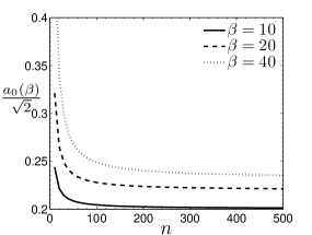
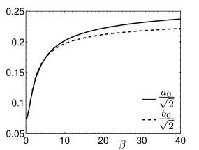
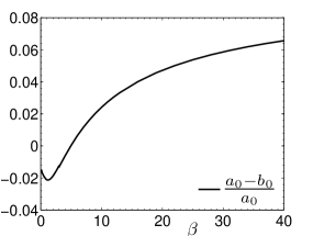
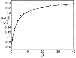
To evaluate $a_{0}(\beta)$ as a function of $\beta$, we solve numerically (85) by truncating the series at sufficiently high values $n$: in Fig. 2(a) we plot the analytic approach result for ${a_{0}(\beta)}/{\sqrt{2}}$ and confirm that it agrees well with results from Brownian simulations that were performed with $\alpha=50$. Interestingly, Fig. 2a shows that the simulation result for $\beta=40$ (when $\beta$ is comparable to $\alpha=50$) still agrees very well with the analytic result derived with the assumption $\alpha\gg\beta$, suggesting that $a_{0}(\beta)$ remains a good approximation until values $\beta\sim\alpha$ ($h\sim R$). As a consequence, this suggests that (90) is an acceptable approximation for $\tau$ until values $h\sim R$. Fig. 2a shows that $a_{0}/\sqrt{2}$ approaches the value $\frac{1}{4}$ for large $\beta$, thus, from (83) we recover the narrow escape formula $\tau\approx\frac{|V|}{4aD}$ [36, 10, 31] derived for a volume with isoperimetric ratio of order 1. Conversely, (81) shows that the validity of the narrow escape formula $\frac{|V|}{4aD}$ is not limited to the range where $h\sim R$, but it is already a valid approximation when $\ln\alpha\ll\beta$ and $\beta\gtrsim 40$ (Fig. 2a). Hence, we conclude that $\tau=\frac{|V|}{4aD}$ is a good approximation even for an oblate volume with $R\gg h$ (and $h\gg a$). In the opposite limit $\beta\to 0$, we find that ${a_{0}(\beta)}/{\sqrt{2}}$ does not converge towards zero (Fig. 2a), but $\lim_{\beta\to 0}{a_{0}(\beta)}/{\sqrt{2}}\approx 0.071$ (in appendix A we derive an analytical approximation for $a_{0}(\beta)$ for $\beta\to 0$). In Fig. 2b we show the effect of the truncation level $n$ on the value of ${a_{0}(\beta)}/{\sqrt{2}}$: after $n\sim 100$ the steady state regime is achieved. Finally, in Fig. 2c-d, we compare the values of the coefficients $a_{0}(\beta)$ and $b_{0}(\beta)$, where $b_{0}(\beta)$ is obtained using (61). The graphs show that $b_{0}(\beta)\approx a_{0}(\beta)$ is a good approximation, and we will use this in section 2.3.3.

Figure 2: (a) Graph of $\frac{a_{0}(\beta)}{\sqrt{2}}$ as a function of $\beta$ for $\alpha\gg 1$. The values for $a_{0}$ are obtained by truncating and numerically solving (85) (for $\beta>10$ we truncate at $n=500$). ${a_{0}(\beta)}/{\sqrt{2}}$ is the average MFPT for Brownian particles starting uniformly distributed at $x=1$. The analytic estimations for ${a_{0}(\beta)}/{\sqrt{2}}$ are compared to results from Brownian simulations (data points) obtained for 10 000 Brownian trajectories, starting uniformly distributed at $x=1$ ( for $\alpha=50$). (b) Dependency of $\frac{a_{0}(\beta)}{\sqrt{2}}$ on the truncation level $n$ for various $\beta$. (c) Comparison between $a_{0}(\beta)$ and $b_{0}(\beta)$, where $b_{0}$ is obtained from (61), showing that $a_{0}(\beta)\approx b_{0}(\beta)$. (d) Relative difference $(a_{0}(\beta)-b_{0}(\beta))/a_{0}(\beta)$.

2.3.2 Boundary layer analysis: particles starting near the absorbing hole

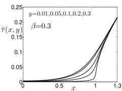
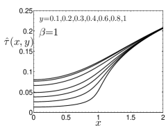
In the neighborhood of the small absorbing window (for $x\sim 1$ and $y\sim 1$), there is a boundary layer (BL) where the behavior of $\hat{\tau}(x,y)$ is very different compared to large $x$ and $y$. In Fig. 3 we study numerically the shape of the BL using (89). The different panels depict $\hat{\tau}(x,y)$ in the neighborhood of the absorbing window for various $\beta$. The plots show that a boundary layer starts to evolve around $\beta\sim 0.3$, and the evolution is almost finished for $\beta\sim 10$ (there is no significant difference between the plots for $\beta=10$ and $\beta=50$). Furthermore, the approximate extent of the boundary layer for large $\beta$ is $\Delta x\sim\Delta y\sim 10$.

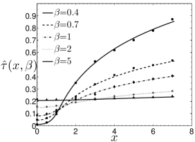
In Fig. 4a, we show $\hat{\tau}(x,\beta)$ for particles released on the upper surface at $y=\beta$ as a function of $x$ and for various $\beta$. Such a situation is relevant at synapses where neurotransmitters are released at the presynaptic terminal, located opposite to the surface with the postsynaptic density (PSD) where receptors are clustered [20, 4]. The hole radius $a$ would correspond to the radius of the PSD. Fig. 4(a) shows that when the height of the synaptic cleft is comparable to the radius of the PSD ($\beta\sim 1)$, $\hat{\tau}(x,\beta)$ changes considerably as a function of the radial release position $x$. In contrast, for $\beta\gg 1$ the release site is outside the boundary layer and the NET is almost independent of $x$ and is well approximated by $1/4$.

Figure 3: Shape of the boundary layer at the absorbing hole for $\alpha\gg 1$ and different values of $\beta$. The NET $\hat{\tau}(x,y)$ (from (89)) as a function of $x$ for different $y$ and $\beta$ (as displayed in each panel).

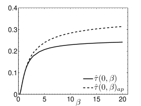
Figure 4: (a) The NET $\hat{\tau}(x,\beta)$ computed from (89) for particles that are released at the upper cylinder surface at radial position $x$ for various $\beta$. We further compare the analytic computations with results from Brownian simulations obtained with 10000 particles and $\alpha=50$. (b) Comparison of $\hat{\tau}(0,\beta)$ with the approximation $\hat{\tau}^{(0)}(0,\beta)_{ap}\approx{a_{0}(\beta)}/{I_{0}(\frac{\pi}{2\beta})}$ given in (95).

2.3.3 Impact of truncating the series for $\hat{\tau}(x,y)$ in(89)

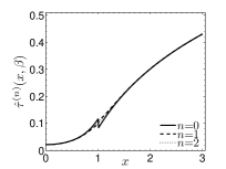
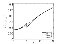
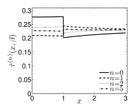
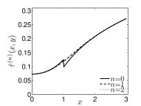
We now study the error induced by truncating the sum in (89) at levels $n\sim 1$ by considering the truncated series

$$\hat{\tau}^{(n)}(x,y)=\left\{\begin{array}[]{l}\displaystyle\sum_{i=0}^{n}b_{i}(\beta)\frac{I_{0}(l_{i}x)}{I_{0}(l_{i})}v_{i}(y)\,,\quad x\leq 1\\ \\ \displaystyle\frac{a_{0}(\beta)}{\sqrt{2}}+\sum_{i=1}^{n}a_{i}(\beta)\frac{K_{0}(k_{i}x)}{K_{0}(k_{i})}u_{i}(y)+\frac{\ln x}{2\pi\beta}\,,\quad 1\leq x\ll\alpha\,,\end{array}\right.$$ (94)

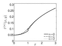
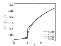
To evaluate the error induced by the truncation, we first compute the coefficients $a_{n}$ and $b_{n}$ with high precision (using a truncation level $n\sim 200$), and then use these values in (94). In Fig. 5, we show the effect of the truncations for various $n$ and $\beta$: interestingly, the numerical analysis reveals that for $\beta\lesssim 1$, truncating at $n=0$ or $n=1$ already provides a very good approximation. The accuracy of the truncation depends on $\beta$, and $n$ has to be increased for larger $\beta$ in order to maintain a similar accuracy (Fig. 5c). In Fig. 4a-c, we plot the effect of the truncation as a function of $x$ for $y=\beta$ (particles are released at the upper surface), and in Fig. 4d-f, the starting position $y$ is reduced to $y=0.7\beta$, $y=0.4\beta$ and $y=0.1\beta$.

Due to the truncation, at the patching boundary $x=1$, (94) has a small discontinuity $\Delta^{(n)}(y)=\hat{\tau}^{(n)}(1^{+},y)-\hat{\tau}^{(n)}(1^{-},y)$. For example, for $n=0$ and $y=\beta$ (see Fig. 5a-c) we obtain $\Delta^{(0)}(\beta)=\frac{a_{0}(\beta)}{\sqrt{2}}-b_{0}(\beta)\approx a_{0}(\beta)(1-\frac{2}{\sqrt{2}})$, where we used $a_{0}(\beta)\approx b_{0}(\beta)$ (see Fig. 2c-d).

Finally, for $\beta\lesssim 1$, when a Brownian particle is released at the center of the upper surface $(x=0,y=\beta)$, using the truncation $n=0$, we obtain from (94)

$$\hat{\tau}(0,\beta)\approx\hat{\tau}^{(0)}(0,\beta)=\frac{b_{0}(\beta)}{I_{0}(\frac{\pi}{2\beta})}\approx\frac{a_{0}(\beta)}{I_{0}(\frac{\pi}{2\beta})}=\frac{\sqrt{2}}{I_{0}(\frac{\pi}{2\beta})}\hat{\tau}(1)\,,$$ (95)

where we additionally used that $a_{0}(\beta\approx b_{0}(\beta)$ and $\hat{\tau}(1)=a_{0}/\sqrt{2}$. In Fig. 4b, we test this approximation as a function of $\beta$ by comparing it with $\hat{\tau}(0,\beta)$, computed with high accuracy ($n\sim 200$). We find that this approximation is valid until $\beta\sim 1$.

(a) $\beta=0.5$

(b) $\beta=1$

(c) $\beta=10$

(d) $\beta=1$ and $y=0.7\times\beta$

(e) $\beta=1$ and $y=0.4\times\beta$

(f) $\beta=1$ and $y=0.1\times\beta$

Figure 5: The truncated NET $\hat{\tau}^{(n)}(x,y)$ from (94) for various truncation levels $n$ and several $\beta$. The figure shows that for $\beta\lesssim 1$ very good results can be obtained by considering a low truncation level $n\sim 2$. (a)-(c): $\hat{\tau}^{(n)}(x,\beta)$ for various $\beta$. (d)-(f): $\hat{\tau}^{(n)}(x,y)$ for $\beta=1$ and various $y$.

2.3.4 Analogy with the electrified disk problem

For $\beta\gg 1$ and $\alpha\gg 1$, an asymptotic solution for $\hat{\tau}(x,y)$ can be obtained by considering the analogy with the electrified disk problem: the total outflux $-1$ through the hole leads to the electrified disk problem with a disk charge $Q=-1$, and using the capacitance $C=4$ of the unit disk [33, 32], we find that the disk potential is ${Q}/{C}=-{1}/{4}$. Using the solution $U(x,y)$ of the electrified disk problem with disk potential $-1/4$ [33], we obtain the asymptotic correspondence

$$\hat{\tau}(x,y)=U(x,y)+\frac{1}{4}\,,\quad\alpha\gg 1\,\,,\beta\gg 1\,.$$ (96)

Hence, for large $\beta$, $U(x,y)$ determines the shape of the boundary layer. Furthermore, by comparing (96) with (89), we recover that $\frac{a_{0}}{\sqrt{2}}=\frac{1}{4}$ for $\beta\sim\alpha\gg 1$.

3 Conditional probability to reach the small target before leaving a laterally open cylinder

When the cylinder is open at the lateral boundary, we shall now compute the conditional probability $p(x,y)$ that a Brownian particle, initially at position $(x,y)$, reaches the small target disk before leaving the cylinder through the lateral opening. Because the geometry of the synaptic cleft can be approximated by a laterally open cylinder [1, 22, 34], we will use our computations to estimate the efficiency of receptor activation at a synapse. Indeed, at the presynaptic site, vesicles release neurotransmitters into the synaptic cleft, and the diffusing neurotransmitter either bind to and thereby activate receptors located on postsynaptic terminal, or they leave the synaptic cleft without activating a receptor. We will first derive a general expression for the conditional probability $p(x,y)$ to hit the small target before exiting, and then compute average values for uniform initial distributions. Finally, we will determine the leading order behavior in a flat cylinder with $R\gg a$ and $h\ll R$.

The conditional probability $p(x,y)$ satisfies the Laplace equation [26, 16]

$$\begin{array}[]{c}\displaystyle\left(\frac{1}{x}\frac{\partial}{\partial x}x\frac{\partial}{\partial x}+\frac{\partial^{2}}{\partial y^{2}}\right)p(x,y)=0\,,\quad x\in\Omega\\ \displaystyle p(x,0)=1\,\mbox{ for }x<1\,,\quad p(x,\alpha)=0\\ \displaystyle\frac{\partial}{\partial y}p(x,0)=0\mbox{ for }1<x<\alpha\,,\quad\displaystyle\frac{\partial}{\partial y}p(x,\beta)=0\,.\end{array}$$ (100)

Similarly to the analysis of $\hat{\tau}(x,y)$ in the previous section, we solve (14) in the subdomains $\Omega_{i}$ and $\Omega_{o}$, and then patch the two solutions $p_{i}(x,y)$ and $p_{o}(x,y)$ at the boundary $x=1$. The general expressions are

$$p(x,y)=\left\{\begin{array}[]{l}\displaystyle 1-\sum_{n=0}^{\infty}b_{n}^{p}\frac{I_{0}(l_{n}x)}{I_{0}(l_{n})}v_{n}(y)\,,\quad x\leq 1\\ \\ \displaystyle\left(1-\frac{a_{0}^{p}}{\sqrt{2}}\right)\frac{\ln\left(\frac{\alpha}{x}\right)}{\ln\alpha}-\sum_{n=1}^{\infty}a_{n}^{p}\frac{G_{0}(k_{n}x,k_{n}\alpha)}{G_{0}(k_{n},k_{n}\alpha)}u_{n}(y)\,,\quad 1\leq x\leq\alpha\end{array}\right.$$ (104)

where

$$G_{0}(x,y)=I_{0}(x)K_{0}(y)-K_{0}(x)I_{0}(y),$$

and the unknown coefficients $a_{n}^{p}$ and $b_{n}^{p}$ are functions of $\alpha$ and $\beta$ and are related by a relation similar to (61). The coefficient $a_{n}^{p}$ resp. $b_{n}^{p}$ are given by

$$\begin{array}[]{lll}\displaystyle\sum_{m=0}^{\infty}(\beta_{n}+\alpha_{m}^{p})\xi_{nm}a_{m}^{p}&=&\displaystyle\xi_{n0}\gamma_{0}^{p}\\ \displaystyle\sum_{m=0}^{\infty}(\beta_{m}+\alpha_{n}^{p})\xi_{mn}b_{m}^{p}&=&\displaystyle\gamma_{0}^{p}\delta_{n0}\,,\end{array}$$ (107)

with

$$\alpha_{0}^{p}=\frac{1}{\ln\alpha}\,,\,\,\alpha_{n}^{p}=-k_{n}\frac{G_{1}(k_{n},k_{n}\alpha)}{G_{0}(k_{n},k_{n}\alpha)}\,(n\geq 1)\,,\quad\beta_{n}=l_{n}\frac{I_{1}(l_{n})}{I_{0}(l_{n})}\,,\quad\gamma_{0}^{p}=\frac{\sqrt{2}}{\ln\alpha}\,,$$ (108)

and

$$G_{1}(x,y)=\frac{\partial}{\partial x}G_{0}(x,y)=I_{1}(x)K_{0}(y)+K_{1}(x)I_{0}(y)\,.$$

For the $\beta_{n}$ we omitted the superscript ^p because they coincide with the $\beta_{n}$ already defined in (64).

3.1 Conditional probabilities with uniform initial distributions

The fraction $p(x)$ of Brownian particles that eventually reach the target starting initially uniformly distributed at $x$ is

$$p(x)=\frac{1}{\beta}\int_{0}^{\beta}p(x,y)dy=\left\{\begin{array}[]{l}\displaystyle 1-\sum_{n=0}^{\infty}\frac{b_{n}^{p}}{\beta l_{n}}\frac{I_{0}(l_{n}x)}{I_{0}(l_{n})}\,,\quad x\leq 1\\ \\ \displaystyle\left(1-\frac{a_{0}^{p}}{\sqrt{2}}\right)\frac{\ln\left(\frac{\alpha}{x}\right)}{\ln\alpha}=p(1)\frac{\ln\left(\frac{\alpha}{x}\right)}{\ln\alpha}\,,\quad 1\leq x\leq\alpha\end{array}\right.$$ (112)

where $p(1)=1-{a_{0}^{p}}/{\sqrt{2}}$. For particles starting initially uniformly distributed in $\Omega$, the average probability is

$$p=\frac{2}{\alpha^{2}}\int_{0}^{\alpha}p(x)xdx=p(1)\frac{\alpha^{2}-2\ln\alpha-1}{2\alpha^{2}\ln\alpha}+\frac{1}{\alpha^{2}}-\frac{2}{\beta\alpha^{2}}\sum_{n=0}^{\infty}\frac{b_{n}}{l_{n}^{2}}\frac{I_{1}(l_{n})}{I_{0}(l_{n})}\,.$$ (113)

When the particles are initially uniformly released at the upper surface within an area $x\leq x_{0}$, the fraction $p_{\beta}(x_{0})$ that will reach the target before escaping through the lateral opening is

$$p_{\beta}(x_{0})=\frac{2}{x_{0}^{2}}\int_{0}^{x_{0}}p(x,\beta)xdx=\left\{\begin{array}[]{l}\displaystyle 1-\frac{2}{x_{0}}\sum_{n=0}^{\infty}(-1)^{n}\frac{b_{n}^{p}\beta_{n}}{l_{n}^{2}}\frac{I_{1}(l_{n}x_{0})}{I_{1}(l_{n})}\,,\quad x_{0}\leq 1\\ \\ \\ \displaystyle\frac{p_{\beta}(1)}{x_{0}^{2}}+\frac{2}{x_{0}^{2}}\left(1-\frac{a_{0}^{p}}{\sqrt{2}}\right)\frac{x_{0}^{2}\left(1+2\ln(\frac{\alpha}{x_{0}})\right)-(1+2\ln\alpha)}{4\ln\alpha}\\ \displaystyle+\frac{2}{x_{0}^{2}}\sum_{n=1}^{\infty}(-1)^{n}\frac{a_{n}^{p}\alpha_{n}^{p}}{k_{n}^{2}}\left(\frac{x_{0}G_{1}(k_{n}x_{0},k_{n}\alpha)}{G_{1}(k_{n},k_{n}\alpha)}-1\right)\,,\quad 1\leq x_{0}\leq\alpha\,.\end{array}\right.$$ (119)

3.2 Asymptotic expressions for the conditional probability in a flat cylinder with $\alpha\gg 1$ and $\beta\ll\alpha$

To obtain an asymptotic expression for the conditional probability $p$ in the limit $\alpha\gg 1$ and $\beta\ll\alpha$, we estimate $a_{n}^{p}$ and $b_{n}^{p}$. For $\alpha\gg 1$ and $\beta/\alpha\ll 1$ we have

$$\alpha_{0}^{p}=\frac{1}{\ln\alpha}\,,\quad\alpha_{n}^{p}\approx k_{n}\frac{K_{1}(k_{n})}{K_{0}(k_{n})}=\alpha_{n},\,\,(n\geq 1)\,,$$

where $\alpha_{n}$ are given in (84). For the scaled coefficients $\tilde{a}_{n}^{p}=\frac{\ln\alpha}{2\pi\beta}a_{n}^{p}$ we obtain from (107) the asymptotic equations

$$(\beta_{n}+\frac{1}{\ln\alpha})\xi_{n0}\tilde{a}_{0}^{p}+\sum_{m=1}^{\infty}(\beta_{n}+\alpha_{m})\xi_{nm}\tilde{a}_{m}^{p}=\frac{1}{\sqrt{2}\pi\beta}\xi_{n0}\,.$$ (120)

When $\alpha$ is large such that $\frac{1}{\ln\alpha}\ll\beta_{n}$, (120) reduces to (85) for the coefficients $a_{n}$ of $\hat{\tau}(x,y)$, hence, $\tilde{a}_{n}^{p}\approx a_{n}$. Because $\beta_{n}$ are monotonically increasing with $n$, if $\frac{1}{\ln\alpha}\ll\beta_{n}$ for $n=0$, this is also valid for $n>0$. Hence, by setting $n=0$, we obtain the condition $\frac{1}{\ln\alpha}\ll\frac{\pi}{2\beta}\frac{I_{1}(\frac{\pi}{2\beta})}{I_{0}(\frac{\pi}{2\beta})}$, satisfied for small $\beta$ when $\ln\alpha\gg\beta$, and for large $\beta$ when $\ln\alpha\gg\beta^{2}$. In this limit, the asymptotic expressions for $a_{n}^{p}$ and $b_{n}^{p}$ are

$$a_{n}^{p}=\frac{2\pi\beta}{\ln\alpha}a_{n}\quad\mbox{and}\quad b_{n}^{p}=\frac{2\pi\beta}{\ln\alpha}b_{n}\,.$$ (121)

Finally, by inserting $a_{n}^{p}$ and $b_{n}^{p}$ into (104) we obtain for for $\ln\alpha\gg\frac{2\beta}{\pi}\frac{I_{0}(\frac{\pi}{2\beta})}{I_{1}(\frac{\pi}{2\beta})}$ the asymptotic formula

$$p(x,y)=\left\{\begin{array}[]{l}\displaystyle 1-\frac{2\pi\beta}{\ln\alpha}\sum_{n=0}^{\infty}b_{n}\frac{I_{0}(l_{n}x)}{I_{0}(l_{n})}v_{n}(y)\,,\quad x\leq 1\\ \\ \displaystyle p(1)\frac{\ln\left(\frac{\alpha}{x}\right)}{\ln\alpha}-\frac{2\pi\beta}{\ln\alpha}\sum_{n=1}^{\infty}a_{n}\frac{K_{0}(k_{n}x)}{K_{0}(k_{n})}u_{n}(y)\,,\quad 1\leq x\ll\alpha\end{array}\right.$$ (125)

where $p(1)=1-\frac{a_{0}^{p}}{\sqrt{2}}=1-\frac{2\pi\beta}{\ln\alpha}\frac{a_{0}}{\sqrt{2}}$ (112) and we used

$$\frac{G_{0}(k_{n}x,k_{n}\alpha)}{G_{0}(k_{n},k_{n}\alpha)}\approx\frac{K_{0}(k_{n}x)}{K_{0}(k_{n})}\,,\quad\alpha\gg 1\mbox{ and }x\ll\alpha\,.$$

By considering (89) for $\hat{\tau}(x,y)$, this can be rewritten as

$$p(x,y)=\left\{\begin{array}[]{l}\displaystyle 1-\frac{2\pi\beta}{\ln\alpha}\hat{\tau}(x,y)\,,\quad x\leq 1\\ \\ \displaystyle 1+\frac{2\pi\beta}{\ln\alpha}\left(1-\frac{\ln\left(\frac{\alpha}{x}\right)}{\ln\alpha}\right)\hat{\tau}(1)-\frac{2\pi\beta}{\ln\alpha}\hat{\tau}(x,y)\,,\quad 1\leq x\ll\alpha\end{array}\right.$$ (129)

showing an interesting relation between the conditional probability and the MFPT. As an example, for particles that start uniformly distributed at $x=1$ we have

$$p(1)=1-\frac{2\pi\beta}{\ln\alpha}\hat{\tau}(1)\,,$$ (130)

and using that $\hat{\tau}(1)\lesssim\frac{1}{4}$, we find that the probability $p(1)$ approaches one for large $\alpha$. In contrast, for particles that start initially uniformly distributed in $\Omega$ we obtain from (113)

$$p\approx\frac{p(1)}{2\ln\alpha}\,,\quad\alpha\gg 1\,,$$ (131)

which shows that $p$ tends to zero for large $\alpha$, in contrast to $p(1)$.

3.3 Numerical evaluations

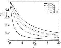
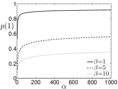
In Fig. 6a we plot $p(1)=1-\frac{a_{0}^{p}}{\sqrt{2}}$ as a function of $\alpha$ for various $\beta$ (we numerically solve (107) with high accuracy up to $n\sim 400$). As $\alpha\to 1$, the probability $p(1)$ tends to zero because the particles start close to the lateral boundary. The asymptotic limit of $p(1)$ for large $\alpha$ is one, as shown in (130). However, the convergence is only logarithmical and therefore very slow. In Fig. 6b we display $p(1)$ as a function of $\beta$ for various $\alpha$: for a fixed value $\alpha>1$, the asymptotic limit of $p(1)$ for $\beta\to 0$ is one, and zero for $\beta\to\infty$. The limit for $\beta\to 0$ is intuitive, because the particles start next to the target. To obtain the asymptotic limit for $\beta\to\infty$ we consider (107) for $a_{n}^{p}$ and (108): because the coefficients $\alpha_{n}^{p}$ ($n\geq 1$) and $\beta_{n}^{p}$ ($n\geq 0$) tend to zero for large $\beta$, the non-vanishing part of (107) is $\alpha_{0}^{p}\xi_{n0}a_{0}^{p}=\gamma_{0}^{p}\xi_{n,0}$, from which it follows that the asymptotic limit of $a_{0}^{p}$ for large $\beta$ is $\sqrt{2}$, and thus $p(1)=1-{a_{0}^{p}}/{\sqrt{2}}$ converges to zero in this limit. Indeed, for fixed $\alpha$ and increasing $\beta$, it becomes less probable that a particle reaches the disk before the lateral boundary.

Figure 6: Average conditional probability $p(1)=1-\frac{a_{0}^{p}}{\sqrt{2}}$ for Brownian particles starting uniformly distributed at $x=1$ to reach the target before leaving the cylinder through the lateral boundary. The coefficient $a_{0}^{p}$ are obtained by truncating and numerically solving (107) with high accuracy. (a) $p(1)$ as a function of $\alpha$ for different $\beta$. (b) $p(1)$ as a function of $\beta$ for different $\alpha$.

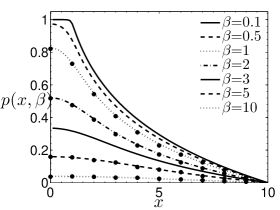
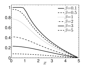
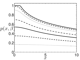
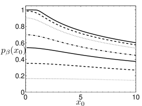
We now study the conditional probability for particles that are released at the upper surface, which is relevant for synaptic transmission. In Fig. 7a-c we plot $p(x,\beta)$ as a function of $x$ for $\alpha=10$, $\alpha=5$ and $\alpha=100$, and various $\beta$ between 0.1 and 10, and in Fig. 7a we further show that our analytical computations agree with results from Brownian simulations. In Fig. 7d we further depict the average probability $p_{\beta}(x_{0})$ when particles are released at the upper surface within an area of radius $x_{0}$ for similar values $\alpha$ and $\beta$ as in panel (c). In general, Fig. 7 shows that $p(x,\beta)$ is very sensitive to the cylinder height $\beta$ and the release position $x$. For very flat cylinders with $\beta\lesssim 1$, when the particles are released in the area opposite to the hole (for $x<1$), the probability is $\sim 1$, whereas when they are released outside this region (for $x>1$), the probability that they reach the target before exiting decreases considerably (Fig. 7a-c). For example, Fig. 7b, obtained for $\beta=0.5$ and $\alpha=5$, shows that the conditional probability is larger than 90% when the particles are released at the upper surface within the area $x<1$, whereas it decreases to around 60% when they are released at $x\sim 2$. For cylinder with large $\alpha$ the impact of the release position is much less pronounced (panel (d) with $\alpha=100$). In addition, Fig. 7 shows that the conditional probability to reach the target is more sensitive to changes in the cylinder height $\beta$ compared to the radius $\alpha$.

(a) $\alpha=10$

(b) $\alpha=5$

(c) $\alpha=100$

(d) $\alpha=100$

Figure 7: Panels a-c: Conditional probability $p(x,\beta)$ (from (104)) for a Brownian particle to reach the target at $(x<1,y=0)$ when released at the upper surface at $y=\beta$ and radial position $x$. The data points in (a) are obtained from Brownian simulations with $10^{3}$ particles. (c) The values for $\beta$ are as in panel (a). (d) Average conditional probability $p_{\beta}(x_{0})$ (from (119)) when the particles are released uniformly on the upper surface in an area of radius $x_{0}$ with values $\beta$ as in (c).

3.4 Impact of truncating the series for $p(x,y)$ in (104)

We now proceed similarly to section 2.3.3 and estimate the error induced by truncating the series in (104) at small $n$. We first compute the coefficients $a_{i}^{p}$ and $b_{i}^{p}$ using (107) with a high accuracy, and then use these coefficients to define the truncated probability

$$p^{(n)}(x,y)=\left\{\begin{array}[]{l}\displaystyle 1-\sum_{i=0}^{n}b_{i}^{p}\frac{I_{0}(l_{i}x)}{I_{0}(l_{i})}v_{i}(y)\,,\quad x\leq 1\\ \\ \displaystyle\left(1-\frac{a_{0}^{p}}{\sqrt{2}}\right)\frac{\ln\left(\frac{\alpha}{x}\right)}{\ln\alpha}-\sum_{i=1}^{n}a_{i}^{p}\frac{G_{0}(k_{i}x,k_{i}\alpha)}{G_{0}(k_{i},k_{i}\alpha)}u_{i}(y)\,,\quad 1\leq x\leq\alpha\end{array}\right.$$ (135)

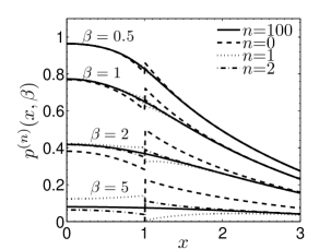
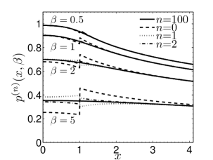
In Fig. 8, we plot $p^{(n)}(x,\beta)$ for various $\alpha$ and $\beta$ as a function of $x$, and show that truncating at $n=0,1,2$ already gives good approximations (we plot $p^{(n)}(x,\beta)$ for $n=100$ to show the error induced by the low truncations). Similarly as in section 2.3.3, we conclude that truncation at $n=1$ or $n=2$ already provides a good approximation for $\beta\lesssim 1$.

(a) $\alpha=5$

(b) $\alpha=100$

Figure 8: The truncated conditional probability $p^{(n)}(x,\beta)$ from (135) for various $n$, $\beta$ and $\alpha$. Similar to Fig. 5, for $\beta\lesssim 1$, we already obtain good approximations for $n\sim 2$.

4 Conditional mean time to reach a small target before escaping a laterally open cylinder

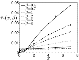
After having estimated the conditional probability $p(x,y)$, we are now in a position to study the conditional MFPT $\hat{\tau}_{c}(x,y)$ to reach a target before escaping through the lateral cylinder boundary. This analysis will estimate the time scale of the synaptic response. For example, the conditional time $\hat{\tau}_{c}(0,\beta)$ in (163) provides an estimate for the mean time until postsynaptic receptors become activated after transmitter release into the synaptic cleft at the upper cylinder surface. In a wide cylinder with $\alpha\gg 1$, (163) shows that the conditional time $\hat{\tau}_{c}(0,\beta)$ is roughly by a factor $1/(\ln\alpha)^{2}$ faster than the mean time $\hat{\tau}(0,\beta)$ for a laterally closed cylinder, because in a closed cylinder all trajectories that are reflected at the lateral boundary contribute to the mean time, thereby increasing the mean compared to an open cylinder. Thus, to obtain a realistic estimation of the synaptic activation time, we have to consider the conditional time $\tau_{c}$ for an open cylinder.

To determine the mean conditional time $\hat{\tau}_{c}(x,y)$, we use the known conditional probability $p(x,y)$ to solve an equation for the function $A(x,y)=\hat{\tau}_{c}(x,y)p(x,y)$, and then we obtain $\hat{\tau}_{c}(x,y)$ from $\hat{\tau}_{c}(x,y)=\frac{A(x,y)}{p(x,y)}$. The function $A(x,y)$ satisfies [9, 35, 17]

$$\begin{array}[]{rcl}\displaystyle\left(\frac{1}{x}\frac{\partial}{\partial x}x\frac{\partial}{\partial x}+\frac{\partial^{2}}{\partial y^{2}}\right)A(x,y)&=&\displaystyle-\frac{p(x,y)}{|\Omega|}\,,\quad(x,y)\in\Omega\\ \displaystyle A(x,y)&=&0\,,\quad y=0\,,x<1\\ \displaystyle A(x,y)&=&0\,,\quad x=\alpha\\ \displaystyle\frac{\partial}{\partial y}A(x,y)&=&0\,,\quad y=0\,,\,x>1\\ \displaystyle\frac{\partial}{\partial y}A(x,y)&=&0\,,\quad y=\beta\,.\end{array}$$ (141)

Proceeding as in the previous sections, we expand $A(x,y)$ as

$$A(x,y)=\left\{\begin{array}[]{l}\displaystyle\sum_{n=0}^{\infty}b^{A}_{n}\frac{I_{0}(l_{n}x)}{I_{0}(l_{n})}v_{n}(y)+w_{i}^{A}(x,y)\,,\quad x\leq 1\\ \\ \displaystyle\frac{a^{A}_{0}}{\sqrt{2}}\frac{\ln\left(\frac{\alpha}{x}\right)}{\ln\alpha}+\sum_{n=1}^{\infty}a^{A}_{n}\frac{G_{0}(k_{n}x,k_{n}\alpha)}{G_{0}(k_{n},k_{n}\alpha)}u_{n}(y)+w_{o}^{A}(x,y)\,,\quad 1\leq x\leq\alpha,\end{array}\right.$$ (145)

where $w_{i}^{A}(x,y)$ and $w_{o}^{A}(x,y)$ are the inhomogeneous solutions of (141) that vanish at $x=1$. The coefficients $a^{A}_{n}$ and $b^{A}_{n}$ are related as $a_{n}$ and $b_{n}$ in (61), and $a^{A}_{n}$ satisfies

$$\sum_{m=0}^{\infty}(\beta_{n}^{A}+\alpha_{m}^{A})\xi_{nm}a^{A}_{m}=\sum_{m=0}^{\infty}\xi_{nm}\gamma_{m}^{A}\,,$$ (146)

where

$$\alpha_{0}^{A}=\frac{1}{\ln\alpha}\,,\,\,\alpha_{n}^{A}=-k_{n}\frac{G_{1}(k_{n},k_{n}\alpha)}{G_{0}(k_{n},k_{n}\alpha)}\,(n\geq 1)\,,\quad\beta_{n}^{A}=l_{n}\frac{I_{1}(l_{n})}{I_{0}(l_{n})}\,,$$ (147)

and the $\gamma_{n}^{A}$ are implicitly defined through

$$\frac{\partial}{\partial x}\left(w_{o}^{A}(x,y)-w_{i}^{A}(x,y)\right)\Big{|}_{x=1}=\sum_{n=0}^{\infty}\gamma_{n}^{A}u_{n}(y)\,.$$ (148)

To determine the coefficients $\gamma^{A}_{n}$, we first evaluate $w_{i}^{A}(x,y)$ and $w_{o}^{A}(x,y)$. When $\alpha\gg 1$, $w_{i}^{A}(x,y)$ is of the order $\alpha^{-2}$ and we neglect its contribution in first approximation. Using $p(x,y)$ from (104), the equation for $w_{o}^{A}(x,y)$ is

$$\begin{array}[]{rcl}\displaystyle\left(\frac{1}{x}\frac{\partial}{\partial x}x\frac{\partial}{\partial x}+\frac{\partial^{2}}{\partial y^{2}}\right)w_{o}^{A}(x,y)&=&\displaystyle-\frac{1}{|\Omega|}\left(p(1)\frac{\ln\left(\frac{\alpha}{x}\right)}{\ln\alpha}-\sum_{n=1}^{\infty}a_{n}^{p}\frac{G_{0}(k_{n}x,k_{n}\alpha)}{G_{0}(k_{n},k_{n}\alpha)}u_{n}(y)\right)\\ \displaystyle w_{o}^{A}(x,y)&=&\displaystyle 0\,,\quad x=1\mbox{ and }x=\alpha\\ \displaystyle\frac{\partial}{\partial y}w_{o}^{A}(x,y)&=&\displaystyle 0\,,\quad y=\beta\mbox{ and }y=0\,.\end{array}$$ (152)

To solve (152) we expand $w_{o}^{A}(x,y)$ in terms of $u_{n}(y)$,

$$w_{o}^{A}(x,y)=w_{o}^{A(0)}(x)+\sum_{n=1}^{\infty}w_{o}^{A(n)}(x)u_{n}(y)\,,$$

and inserting this expansion into (152) gives for $w_{o}^{A(0)}(x)$ the solution

$$w_{o}^{A(0)}(x)=-\frac{p(1)}{4|\Omega|\ln(\alpha)}\left(x^{2}(\ln\left(\frac{\alpha}{x}\right)+1)-(\alpha^{2}-\ln\alpha-1)\frac{\ln x}{\ln\alpha}-(\ln\alpha+1)\right)\,.$$ (153)

The higher order functions $w_{o}^{A(n)}(x)$ ($n\geq 1$) satisfy the equation

$$\begin{array}[]{c}\displaystyle\left(\frac{1}{x}\frac{\partial}{\partial x}x\frac{\partial}{\partial x}-k_{n}^{2}\right)w_{o}^{A(n)}(x)=\displaystyle\frac{a_{n}^{p}}{|\Omega|}\frac{G_{0}(k_{n}x,k_{n}\alpha)}{G_{0}(k_{n},k_{n}\alpha)}\,,\quad 1<x<\alpha\\ \displaystyle w_{o}^{A(n)}(1)=0\,,\quad\displaystyle w_{o}^{A(n)}(\alpha)=0\,.\end{array}$$

To proceed, we now truncate the series for $w_{o}^{A}(x,y)$ in (4) at $n=0$ and use only the first order approximation $w_{o}^{A}(x,y)\approx w_{o}^{A(0)}(x)$. We expect that this already provides a good approximation because the coefficients $a_{n}^{p}$ are small for for $n\geq 1$ and large $\alpha$, and, as shown in section 3.4, truncation at $n=0$ already gives a very good approximation for $p(x,y$ when $\beta\lesssim 1$. Hence, we expect that our analysis is a valid approximation for large $\alpha$ and small $\beta\sim 1$. With truncation at $n=0$, the parameters $\gamma_{n}^{A}$ defined in (148) are

$$\gamma_{n}^{A}=\gamma_{0}^{A}\delta_{n0}\,,\quad\mbox{with}\quad\gamma_{0}^{A}=p(1)\frac{\alpha^{2}-2(\ln\alpha)^{2}-2\ln\alpha-1}{2\sqrt{2}\pi\beta\alpha^{2}(\ln\alpha)^{2}}\approx\frac{1}{\sqrt{2}\pi\beta}\frac{p(1)}{2(\ln\alpha)^{2}}\,.$$ (156)

Similar to (121), for $\displaystyle{\ln\alpha\gg\frac{2\beta}{\pi}\frac{I_{0}(\frac{\pi}{2\beta})}{I_{1}(\frac{\pi}{2\beta})}}$, the asymptotic solutions for $a_{n}^{A}$ and $b_{n}^{A}$ in terms of $a_{n}$ and $b_{n}$ are

$$a_{n}^{A}=\frac{p(1)}{2(\ln\alpha)^{2}}a_{n}\quad\mbox{and}\quad b_{n}^{A}=\frac{p(1)}{2(\ln\alpha)^{2}}b_{n}\,.$$ (157)

Finally, we obtain for $\hat{\tau}_{c}(x,y)$ the approximation

$$\hat{\tau}_{c}(x,y)=\frac{A(x,y)}{p(x,y)}=\frac{1}{p(x,y)}\left\{\begin{array}[]{l}\displaystyle\sum_{n=0}^{\infty}b_{n}^{A}\frac{I_{0}(l_{n}x)}{I_{0}(l_{n})}v_{n}(y)=\frac{p(1)}{2(\ln\alpha)^{2}}\hat{\tau}(x,y)\,,\quad x\leq 1\\ \\ \displaystyle\frac{a^{A}_{0}}{\sqrt{2}}\frac{\ln\left(\frac{\alpha}{x}\right)}{\ln\alpha}+\sum_{n=1}^{\infty}a_{n}^{A}\frac{K_{0}(k_{n}x)}{K_{0}(k_{n})}u_{n}(y)+w_{o}^{A(0)}(x)\,,\quad 1\leq x\ll\alpha\end{array}\right.$$ (161)

where $p(x,y)$ is given in (125). To estimate how much $\hat{\tau}_{c}(x,y)$ is faster compared to $\hat{\tau}(x,y)$, we consider particles that are released centrally on the upper surface at position $(0,\beta)$. By taking into account (129) for $p(x,y)$, we obtain

$$\hat{\tau}_{c}(0,\beta)=\frac{1-\frac{2\pi\beta}{\ln\alpha}\hat{\tau}(1)}{1-\frac{2\pi\beta}{\ln\alpha}\hat{\tau}(0,\beta)}\frac{\hat{\tau}(0,\beta)}{2(\ln\alpha)^{2}}\,.$$ (162)

Furthermore, using from (95) the approximation $\hat{\tau}(0,\beta)\approx\frac{a_{0}(\beta)}{I_{0}(\frac{\pi}{2\beta})}=\frac{\sqrt{2}}{I_{0}(\frac{\pi}{2\beta})}\hat{\tau}(1)$, we obtain for $\beta\lesssim 1$ the approximation

$$\hat{\tau}_{c}(0,\beta)\approx\frac{1-\frac{\sqrt{2}\pi\beta}{\ln\alpha}I_{0}(\frac{\pi}{2\beta})\hat{\tau}(0,\beta)}{1-\frac{2\pi\beta}{\ln\alpha}\hat{\tau}(0,\beta)}\frac{\hat{\tau}(0,\beta)}{2(\ln\alpha)^{2}}\,.$$ (163)

In Fig. 9 we plot a $\hat{\tau}_{c}(x,\beta)$ as a function of $x$ for various $\beta$, and we confirm that our analysis agrees well with results from Brownian simulations. Comparing Fig. 9 with Fig. 4 for $\hat{\tau}(x,y)$ shows that $\hat{\tau}_{c}(x,\beta)$ is roughly by a factor $(2\ln\alpha)^{2}$ faster compared to $\hat{\tau}(x,y)$.

Figure 9: Conditional MFPT $\hat{\tau}_{c}(x,\beta)$ to reach the hole in a laterally open cylinder for particles that are released on the surface opposed to the hole. The numerical values for $\hat{\tau}_{c}(x,\beta)$ are calculated using (161) and $\alpha=50$. The data points are the results of Brownian simulations with 10000 particles and $\alpha=50$.

5 Discussion and conclusion

We generalized here the narrow escape problem to a degenerated geometry defined by a flat cylindrical compartment of height $h$ and radius $R$, where the absorbing hole is a small circular disk of radius $a$ located centrally on the lower surface. We analyzed the problem for a laterally closed and open cylinder. Because a uniform analytic expansion of the solution in the whole domain is not possible, we derived two different expansions in the two subregions $\Omega_{i}$ and $\Omega_{o}$, and then matched them at the boundary between the two subcompartments.

We first analyzed the narrow escape time (NET) $\tau(r,z)$ to reach the small hole in a laterally closed cylinder. For a flat cylinder with $h\ll R$ and $R\gg a$, we obtained that the NET (90) is given by

$$\tau\approx\frac{|V|}{aD}\frac{a_{0}\left(\frac{h}{a}\right)}{\sqrt{2}}+\frac{R^{2}}{8D}\left(4\ln\left(\frac{R}{a}\right)-3\right)\,,$$ (164)

where the function $a_{0}(\beta)\in[0.07,0.25]$ (Fig. 2a). Although (164) was derived in the condition that $h\ll R$, our numerical results suggest that it remains valid until $h\sim R$ (section 2.3.1). In particular, for a cylinder with $h/a\gg\ln\left(\frac{R}{a}\right)$ we recover the well known NET approximation $\tau\approx\frac{|V|}{4aD}$ [36, 10, 14], which was derived for non degenerated geometries (isoperimetric ratio of order 1 and no bottle neck). However, our analysis for the cylinder revealed that $\tau=\frac{|V|}{4aD}$ is already a very good approximation for an oblate volume with an isoperimetric ratio that can be very different from 1 (although $h/a\gg\ln\left(\frac{R}{a}\right)$, the ratio $h/R$ can still be small). Formula 164 can also be used to estimate the rate constant of a key chemical reaction during the early stage of phototransduction, which is the rate for diffusing cGMP molecules to reach the phosphodiesterase enzyme located on the surface of a narrow cylinder, located in the outer segment of a rod photoreceptor [23, 24].

In a next step, we used our method to analyze the narrow escape problem for a flat and laterally open cylinder, which is relevant for synaptic transmission. In many cases, the geometry of the synaptic cleft is well approximated by a laterally open cylinder [1, 22, 34], where neurotransmitters are released into the synaptic cleft from the presynaptic terminal, located on the upper surface. The neurotransmitters move in the synaptic cleft (Fig. 1) by Brownian diffusion, and they either activate receptors clustered in the postsynaptic density located on the postsynaptic terminal (corresponding to the lower cylinder surface), or they leave the synaptic cleft through the lateral boundary without binding to a receptor.

We estimated the conditional probability $p(r,z)$ that a particle starting at position $(r,z)$ reaches the small hole before leaving the cylinder. By identifying the small hole with the postsynaptic density where receptors are clustered, we estimated the fraction of released neurotransmitters that reach the receptor area before leaving the synaptic cleft. Using our analytic solution, we studied the impact of the synaptic cleft geometry as well as the location of neurotransmitter release. In Fig. 7, we plotted the probability to reach the postsynaptic density before leaving as a function of the release position for various cylinder height, and we found that it is very sensitive to the release position and the width of the cylinder. We conclude that, in order to achieve an efficient activation of postsynaptic receptors, the presynaptic and postsynaptic densities should be properly aligned such that the neurotransmitters are released opposite to the receptors. Finally, we computed the conditional mean time to reach the small hole before leaving through the lateral boundary (see (161)). For a wide cylinder, we found that the conditional mean time is roughly by a factor $(2\ln\alpha)^{2}$ faster compared to the NET in a closed cylinder (see (163)).

We shall now present some numerical estimates for neurotransmitters that need to activate receptors clustered in the postsynaptic density with a radius $a=50nm$, when the synaptic cleft has a height $h=20nm$ and a total radius of $R=500nm$, so that $\alpha=R/a=10$ and $\beta=h/a=0.4$. When the transmitter are released at distance $r$ away from the center, the conditional probability is approximately given by truncating (104) at $n=0$

$$p(r,h)=\left\{\begin{array}[]{l}\displaystyle 1-b_{0}^{p}\frac{I_{0}(\frac{\pi r}{2h})}{I_{0}(\frac{a\pi}{2h})}\,,\quad x\leq 1\\ \\ \displaystyle\left(1-\frac{a_{0}^{p}}{\sqrt{2}}\right)\frac{\ln\left(\frac{R}{r}\right)}{\ln R/a}\,,\quad 1\leq r\leq R\end{array}\right.$$ (168)

which is a very good approximation, as shown in Fig. 8. Using a diffusion constant $D=200\mu m^{2}/s$, we obtain for the mean times $\tau(0,h)\approx 17\mu s$ and $\tau_{c}(0,h)=1\mu s$.

The exact solution for the mean time and the conditional probability were obtained here by using the patching eigenfunction expansion approach, and from these approximations, we derived in the limit of large aspect ratio $R/h\gg 1$ the asymptotic behavior. Our approach works well because of the radial symmetry due to the absorbing trap that is is located at the center of the cylinder. This situation accounts well for the postsynaptic density located at the center of the post-synaptic terminal. However, using our method it would be difficult to treat the case of multiple non-concentric traps, and in this case a different approach based on matching asymptotic analysis should be more appropriate [21, 6]. The analysis should start with an explicit representation of the Green’s function for a cylinder. Once an inner solution is determined near each trap, it should be matched to the outer solution [21]. This method should allow to study the effect of the trap positions and trap clustering on the synaptic current, which was only partially discussed in [34, 15].

Acknowledgements

D.H. research is supported by an ERC Starting Grant.

APPENDIX

Appendix A Equation for the parameters $a_{n}$ in the limit $\beta\ll 1$

In order to find the asymptotic equations for the coefficients $a_{n}$ for $\alpha\gg 1$ and $\beta\to 0$, we introduce the scaled quantities

$$\begin{array}[]{c}\displaystyle\hat{l}_{n}=\beta l_{n}=\frac{(2n+1)\pi}{2}\,,\quad\hat{k}_{n}=\beta k_{n}=n\pi\,,\\ \displaystyle\hat{\beta}_{n}=\beta\beta_{n}=\hat{l}_{n}\frac{I_{1}(l_{n})}{I_{0}(l_{n})}\,,\quad\hat{\alpha}_{n}=\beta\alpha_{n}=\hat{k}_{n}\frac{K_{1}(k_{n})}{K_{0}(k_{n})}\,,\quad\hat{\gamma}_{0}=\beta\gamma_{0}=\frac{1}{\sqrt{2}\pi}\,.\end{array}$$

In the limit $\beta\to 0$ we have $l_{n}\to\infty$ and $k_{n}\to\infty$ for every $n>0$, and the asymptotic behaviour of $\hat{\beta}_{n}$ and $\hat{\alpha}_{n}$ is

$$\begin{array}[]{c}\hat{\beta}_{n}\approx\hat{l}_{n}\,,\quad n\hat{\alpha}_{n}\approx\hat{k}_{n}\end{array}$$ (172)

Using (85), the asymptotic equation for the coefficients $a_{n}$ in the limit $\beta\to 0$ is

$$\sum_{m=0}^{\infty}(\hat{l}_{n}+\hat{k}_{m})\xi_{nm}a_{m}=\frac{1}{\sqrt{2}\pi}\xi_{n0}\,.$$ (173)

Truncating (173) at various levels $n$ gives the approximations

$$\frac{a_{0}}{\sqrt{2}} = \frac{1}{\pi^{2}}\approx 0.10\,,\quad n=0$$

$$\frac{a_{0}}{\sqrt{2}} = \frac{5}{6}\frac{1}{\pi^{2}}\approx 0.085\,,\quad n=1$$

$$\frac{a_{0}}{\sqrt{2}} = \frac{47}{60}\frac{1}{\pi^{2}}\approx 0.078\,,\quad n=2\,.$$

Numerically we find from (173)

$$\frac{a_{0}}{\sqrt{2}}\approx 0.071$$ (174)

References

• [1] B. Barbour. An evaluation of synapse independence. J. Neuroscience, 21(20):7969–7984, 2001.
• [2] H. C. Berg and M. Purcell. Physics of chemoreception. Biophys. J., 20:193–219, 1977.
• [3] J.N. Bourne and K.M. Harris. Balancing structure and function at hippocampal dendritic spines. Annu. Rev. Neurosci., 31:47–67, 2008.
• [4] Harris K.M. Bourne J.N. Balancing structure and function at hippocampal dendritic spines. Annu Rev Neurosci., 31:47–67, 2008.
• [5] H.S. Carslaw and J.C. Jaeger. Conduction of Heat in Solids. Oxford University Press, USA, 2 edition edition, 1986.
• [6] A.F. Cheviakov, M.J. Ward, and R. Straube. An asymptotic analysis of the mean first passage time for narrow escape problems: Part ii: The sphere. SIAM Multiscale Modeling and Simulation, 8:836–870, 2010.
• [7] S. Condamin, O. Bénichou, V. Tejedo, R. Voituriez, and J. Klafter. First-passage times in complex scale-invariant media. Nature, 450(7166):77–80, 2007.
• [8] G.M. Elias and Nicoll R.A. Synaptic trafficking of glutamate receptors by maguk scaffolding proteins. Trends Cell Biol., 7:343–52, 2007.
• [9] C.W. Gardiner. Handbook of Stochastic Methods. Springer, third edition, 2003.
• [10] I. V. Grigoriev, Y. A. Makhnovskii, A. M. Berezhkovskii, and V. Yu. Zitserman. Kinetics of escape through a small hole. J. Chem. Phys., 116:9574–77, 2002.
• [11] D Holcman. Modeling viral and dna trafficking in the cytoplasm of a cell. J. of Stat. Phys., 127(3):471–494, 2007.
• [12] D Holcman. Computational challenges in synaptic transmission. Book Series: Contemporary Mathematics; Source: Imaging Microstructures: Mathematical and Computational challenges, 494:1–26, 2009.
• [13] D. Holcman and J.I. Korenbrot. Longitudinal diffusion in retinal rod and cone outer segment cytoplasm: The consequence of the cell structure. Biophys. J., 86:2566–2582, 2004.
• [14] D. Holcman and Z. Schuss. Escape through a small opening: receptor trafficking in a synaptic membrane. J. Stat. Phys., 117(5/6):975–1014, 2004.
• [15] D. Holcman and Z. Schuss. Diffusion through a cluster of small windows and flux regulation in microdomains. Phys. Lett. A., 372(21):3768–72, 2008.
• [16] S. Karlin and H.M. Taylor. A First Course in Stochastic Processes. Academic Press, 2. edition edition, 1975.
• [17] S. Karlin and H.M. Taylor. A Second Course in Stochastic Processes. Academic Press, 1 edition edition, 1981.
• [18] T. Lagache, E. Dauty, and D. Holcman. Physical principles and models describing intracellular virus particle dynamics. Curr. Opin. Microbiol., 12(4):439–445, 2009.
• [19] T. Lagache and D. Holcman. Quantifying intermittent transport in cell cytoplasm. Phys. Rev. E, 77(3):030901, 2008.
• [20] T.M. Newpher and M.D. Ehlers. Glutamate receptor dynamics in dendritic microdomains. Neuron, 58(4):472–97, 2008.
• [21] S. Pillay, M.J. Ward, A. Peirce, and T. Kolokolnikov. An asymptotic analysis of the mean first passage time for narrow escape problems: Part i: Two-dimensional domains. SIAM Multiscale Modeling and Simulation, 8:803–835, 2010.
• [22] S. Raghavachari and J.E. Lisman. Properties of quantal transmission at ca1 synapses. J. Neurophysiology, 92(4):2456–2467, 2004.
• [23] J. Reingruber and D Holcman. Estimating the rate of cgmp hydrolysis by phosphodiesterase in photoreceptors. J. Chem. Phys., 129:145192, 2008.
• [24] J. Reingruber and D Holcman. Diffusion in narrow domains and application to phototransduction. Phys. Rev. E, 79(3):030904, 2009.
• [25] F. Rieke and D. Baylor. Single photon detection by rod cells of the retina. Rev. of Mod. Phys., 70(3):1027–1036, 1998.
• [26] Z. Schuss. Theory and Applications of Stochastic Differential Equations. Wiley Series in Probability and Statistics, John Wiley Sons, Inc., New York, 1980.
• [27] Z. Schuss, A. Singer, and D Holcman. The narrow escape problem for diffusion in cellular microdomains. Proc. Natl. Acad. Sci. USA, 104(41):16098–103, 2007.
• [28] A. Singer and Z. Schuss. Activation through a narrow opening. Phys. Rev. E, 74(2):020103, 2006.
• [29] A. Singer, Z. Schuss, and D Holcman. Narrow escape iii. J. Stat. Phys., 122(3):491–509, 2006.
• [30] A. Singer, Z. Schuss, and D. Holcman. Narrow escape and leakage of brownian particles. Phys. Rev. E, 78(5):051111, 2008.
• [31] A. Singer, Z. Schuss, D. Holcman, and B. Eisenberg. Narrow escape i. J. Stat. Phys., 122(3):437–536, 2006.
• [32] W. R. Smythe. Static and dynamic electricity. McGraw-Hill Book Company, Inc., New York Toronto London, 1950.
• [33] I. Sneddon. Mixed boundary value problems in potential theory. John Wiley Sons, Inc., New York, 1966.
• [34] A. Taflia and D Holcman. Estimating the synaptic current in a multi-conductance ampa receptor model. arXiv:1009.0867v1 [q-bio.NC].
• [35] A. Taflia and D Holcman. Dwell time of a brownian molecule in a microdomain with traps and a small hole on the boundary. J. Chem. Phys., 126(23):234107, 2007.
• [36] M.J. Ward and J.B. Keller. Strong localized perturbations of eigenvalue problems. SIAM J. Appl. Math., 53:770–798, 1993.
• [37] M.J. Ward and E. Van De Velde. The onset of thermal runaway in partially insulated or cooled reactors. IMA J. Appl. Math., 48:53–83, 1992.
• [38] G. Wilemski and M. Fixman. General theory of diffusion-controlled reactions. J. Chem. Phys., 58:4009, 1973.
• [39] R. Zwanzig. Diffusion-controlled ligand binding to spheres partially covered by receptors: An effective medium traetment. Proc. Natl. Acad. Sci. USA, 87:5856–5857, 1990.