Future weak lensing constraints in a dark coupled universe

Abstract

Coupled cosmologies can predict values for the cosmological parameters at low redshifts which may differ substantially from the parameters values within non-interacting cosmologies. Therefore, low redshift probes, as the growth of structure and the dark matter distribution via galaxy and weak lensing surveys constitute a unique tool to constrain interacting dark sector models. We focus here on weak lensing forecasts from future Euclid and LSST-like surveys combined with the ongoing Planck cosmic microwave background experiment. We find that these future data could constrain the dimensionless coupling to be smaller than a few $\times 10^{-2}$. The coupling parameter $\xi$ is strongly degenerate with the cold dark matter energy density $\Omega_{c}h^{2}$ and the Hubble constant $H_{0}$. These degeneracies may cause important biases in the cosmological parameter values if in the universe there exists an interaction among the dark matter and dark energy sectors.

I Introduction

Cosmological probes indicate that the universe we observe today possesses a flat geometry and a mass energy density made of $\sim 30\%$ baryonic plus cold dark matter and $70\%$ dark energy, responsible for the late-time accelerated expansion wmap7 ; sdss2 ; snalate . While the $\Lambda$CDM model (a flat universe with a cosmological constant) can describe the current observational data, there exist also dynamical options for dark energy, as the quintessence fluid, in which a cosmic scalar field is slowly approaching its ground state. This quintessence field, in principle, may couple to other fields in nature. Observations strongly constrain the couplings to ordinary matter Carroll:1998zi . However, interactions within the dark sectors, i.e. between dark matter and dark energy, are still allowed by observations Amendola:1999er ; Amendola:1999dr ; Amendola:1999qq ; Amendola:2000uh ; Amendola:2003wa ; Amendola:2006dg ; Valiviita:2008iv ; He:2008si ; Jackson:2009mz ; Gavela:2009cy ; CalderaCabral:2009ja ; Valiviita:2009nu ; Majerotto:2009np ; Gavela:2010tm ; Honorez:2010rr ; Martinelli:2010rt ; LopezHonorez:2010ij . Coupled cosmologies, in order to satisfy CMB constraints, predict values for the cosmological parameters today which may differ substantially from the parameters values within non-interacting cosmologies. Therefore interacting cosmologies can hide their effects at low redshifts and weak lensing measurements can help enormously in constraining dark sector coupled models.

We review here the future CMB constraints on interacting dark matter-dark energy models presented in Ref. Martinelli:2010rt , adding weak lensing data from the future Euclid Refregier:2006vt ; Refregier:2010ss and LSST :2009pq -like surveys. Weak lensing probes are shown to be highly complementary to CMB measurements and extremely powerful tools to constrain interacting dark sector models.

The structure of the paper is as follows. Section II presents the basics of coupled cosmologies. In Secs. III and IV we describe the lensing extraction methods for galaxy surveys and CMB measurements respectively. Section V contains the description of the future data used in our analyses. The results from our Markov Chain Monte Carlo (MCMC) analyses are presented in Sec. VI. We draw our conclusions in Sec. VII.

II Coupled cosmologies

At the level of the stress-energy tensor it is always possible to introduce an interaction between the fluids of the dark sector in the following way Kodama:1985bj :

$$\nabla_{\mu}T^{\mu}_{({\rm dm})\nu}=Q_{\nu}\quad\mbox{and}\quad\nabla_{\mu}T^{\mu}_{({\rm de})\nu}=-Q_{\nu}.$$ (1)

The 4-vector $Q_{\nu}$ governs the energy-momentum transfer between the dark components and $T^{\mu}_{({\rm dm})\nu}$ and $T^{\mu}_{({\rm de})\nu}$ are the energy-momentum tensors for the dark matter and dark energy fluids, respectively. The momentum exchange $Q_{\nu}$ can be parallel to the dark energy four velocity $u_{\nu}^{({\rm de})}$ or to the dark matter four velocity $u_{\nu}^{({\rm dm})}$. The first option include all quintessence coupled models and are effectively “modified gravity” models, implying the presence of a “fifth force” effect (only for the dark matter), that is, a violation of the equivalence principle. For both options the evolution equations for the dark matter and dark energy background energy densities are identical and reduce to:

$$\dot{\bar{\rho}}_{\rm dm}+3\mathcal{H}\bar{\rho}_{\rm dm} = a\bar{Q}\,,$$ (2)

$$\dot{\bar{\rho}}_{\rm de}+3\mathcal{H}\bar{\rho}_{\rm de}(1+w) = -a\bar{Q}\,,$$ (3)

where the bars denote background quantities, the dot indicates derivative with respect to conformal time $d\tau=dt/a$, $\mathcal{H}={\dot{a}}/a$ and $w$ is the dark-energy equation of state. For $Q>0$, the energy flows from the dark energy system to dark matter one. For $Q<0$, the energy flow is reversed. In coupled cosmologies the momentum exchange can be proportional to the dark matter energy density ($Q\propto\rho_{\rm dm}$) or proportional to the dark energy energy density ($Q\propto\rho_{\rm de}$). . However, even if models proportional to the dark matter and dark energy velocities provide the same background history, the perturbation evolution is dramatically different. Therefore, while geometrical probes alone are unable to distinguish among the two of them, probes of the perturbation evolution via weak lensing measurements will make these two models fundamentally different. Another aspect of coupled models is that they can show non adiabatic, early time instabilities Valiviita:2008iv ; He:2008si ; Chongchitnan:2008ry ; Gavela:2009cy ; Jackson:2009mz ; Corasaniti:2008kx ; Majerotto:2009np due to the dark coupling term which appears in the dark energy pressure perturbations. In the following, we shall restrict our analyses to coupled models which satisfy the stability criterion of Ref. Gavela:2009cy and therefore are free of early-time, non adiabatic instabilities. We consider the dark coupled model of Ref. Gavela:2009cy (see also Ref. Gavela:2010tm for the perturbation analysis details)

$$Q_{\nu}^{({\rm dm})}=\xi H\rho_{\rm de}u_{\nu}^{({\rm dm})}=-Q_{\nu}^{({\rm de})}~{},$$ (4)

where $\xi$ is a dimensionless coupling (considered constant, as well as the dark energy equation of state $w$, in the present analysis). $H$ and $\rho_{\rm de}$ refer to the total expansion rate and dark energy density, background plus perturbation, i.e $H={\cal H}/a+\delta H$ and $\rho_{\rm de}=\bar{\rho}_{\rm de}+\delta\rho_{\rm de}$ respectively. Notice from Eq. (4) that $Q_{\nu}^{({\rm a})}$ has been chosen parallel to the dark matter four velocity $u_{\nu}^{({\rm dm})}$, in order to avoid momentum transfer in the rest frame of the dark matter component Valiviita:2008iv . For this choice of energy exchange $Q_{\nu}^{({\rm a})}$, positive (negative) values of the coupling $\xi$ will lead to lower (higher) dark matter energy densities in the past than in the uncoupled $\xi=0$ case. We only consider here negative couplings and $w>-1$, avoiding the instability problems previously mentioned, see Ref. Gavela:2009cy for details. For the numerical analyses presented here, we have modified the publicly available CAMB code camb , taking into account the presence of the dark coupling in both the background and the linear perturbation equations.

III Galaxy weak Lensing

Weak gravitational lensing of the images of distant galaxies offers a useful geometrical way to map the matter distribution in the Universe. Following Ref. Bartelmann:1999yn one can describe the distortion of the images of distant galaxies through the tensor:

$\psi_{ij}=\left(\begin{array}[]{cc}-\kappa-\gamma_{1}&-\gamma_{2}\\ -\gamma_{2}&-\kappa+\gamma_{2}\\ \end{array}\right)$

where $\kappa$ is the convergence term and $\gamma=\gamma_{1}+i\gamma_{2}$ is the complex shear field. As shown in Ref. Huterer:2010hw the shear and the convergence terms can be written as a function of the projected Newtonian potentials $\psi_{,ij}$:

$$\gamma=\frac{1}{2}(\psi_{,11}-\psi_{,22})+i\psi_{,12}\ ,$$

$$k=\frac{1}{2}(\psi_{,11}-\psi_{,22})$$

where the commas indicate the derivatives with respect to the directions transverse to the line of sight and the projected potentials are $\psi_{,ij}=-(1/2)\int g(z)(\Psi_{,ij}+\Phi_{,ij})dz$ with the lensing kernel :

$$g(z)=\int dz^{\prime}\frac{n(z^{\prime})D_{A}(z,z^{\prime})}{D_{A}(0,z^{\prime})}\ .$$

Here $n(z)$ is the galaxy redshift distribution. In our analysis we assume flatness of the Universe. However in general the angular diameter distance $D_{A}$ between the lens and the source depends on the spatial curvature $K$:

$$D_{A}=\frac{1}{\sqrt{K}}\sin(\sqrt{K}r),\phantom{aaa}K>0$$

$$D_{A}=r,\phantom{aaa}K=0$$

$$D_{A}=\frac{1}{\sqrt{-K}}\sinh(\sqrt{-K}r),\phantom{aaa}K<0$$

and the comoving distance is:

$$r(z,z^{\prime})=\int_{z}^{z^{\prime}}\frac{dz^{\prime}}{E(z^{\prime})}$$

with $E(z)=H(z)/H_{0}$.

Images distortions induced by the matter distribution are generally small. To extract cosmological information it is hence necessary to statistically analyze a large number of images. The two point correlation function of the convergence is at present the best measured statistic of the weak lensing but, of course, also higher order statistics contains cosmological information. It is convenient to work in the multipole space and define the convergence power spectrum as the harmonic transform of the two-point correlation function. This is usually the most analyzed and studied statistical quantity related to the weak lensing and we will focus on the convergence power spectra in order to properly compare our results to similar analysis in literature. However it should be stressed that, as shown in Schneider:2002jd , the convergence power spectrum is only indirectly and partially obtainable from the two point correlation function.

Future surveys will measure redshifts of billions of galaxies allowing the possibility of a tomographic reconstruction of the matter distribution. We can define hence the convergence power spectra in each redshift bin and the cross-power spectra:

$$P_{jk}(\ell)=H_{0}^{3}\int_{0}^{\infty}\frac{dz}{E(z)}W_{i}(z)W_{j}(z)P_{NL}[P_{L}\left(\frac{H_{0}\ell}{r(z)},z\right)]$$ (5)

where $P_{NL}$ is the non-linear matter power spectrum at redshift $z$, obtained correcting the linear one $P_{L}$. $W(z)$ is a weighting function:

$$W_{i}(z)=\frac{3}{2}\Omega_{m}(1+z)\int_{z_{i}}^{z_{i+1}}dz^{\prime}\frac{n_{i}(z^{\prime})r(z,z^{\prime})}{r(0,z^{\prime})}$$ (6)

with subscripts $i$ and $j$ indicating the redshift bin. Equation (5) shows the cosmological information contained in weak lensing measurements: the function $W(z)$ encodes the information on how the three-dimensional matter distribution is projected on the sky, while the matter power spectrum quantifies the overall matter distribution.
The observed convergence power spectra is affected mainly by systematic uncertainties arising from the intrinsic ellipticity of galaxies $\gamma^{2}_{rms}$. These uncertainties can be reduced averaging over a large number of sources. The observed convergence power spectra will be hence:

$$C_{jk}=P_{jk}+\delta_{jk}\gamma^{2}_{rms}\tilde{n}_{j}^{-1}$$ (7)

where $\tilde{n}_{j}$ is the number of sources per steradian in the $j-th$ bin.

IV CMB Lensing extraction

The analysis presented here includes, in addition to the primary CMB anisotropy angular power spectrum, the information from CMB lensing. Gravitational CMB lensing, as already shown (see e.g. Perotto:2006rj ; Calabrese:2009tt ) can improve significantly the CMB constraints on several cosmological parameters, since it is strongly connected with the growth of perturbations and gravitational potentials at redshifts $z<1$ and therefore, it can break important degeneracies. The lensing deflection field $d$ can be related to the lensing potential $\phi$ as $d=\nabla\phi$ hirata:2003 . In harmonic space, the deflection and lensing potential multipoles follow

$$d_{l}^{m}=-i\sqrt{l(l+1)}\phi_{l}^{m},$$ (8)

and therefore, the power spectra $C^{dd}_{l}\equiv\left\langle d_{l}^{m}d_{l}^{m*}\right\rangle$ and $C_{l}^{\phi\phi}\equiv\left\langle\phi_{l}^{m}\phi_{l}^{m*}\right\rangle$ are related through

$$C_{l}^{dd}=l(l+1)C_{l}^{\phi\phi}.$$ (9)

Lensing introduces a correlation between different CMB multipoles (that otherwise would be fully uncorrelated) through the relation

$$\left\langle a_{l}^{m}b_{l^{\prime}}^{m^{\prime}}\right\rangle=(-1)^{m}\delta_{m}^{m^{\prime}}\delta_{l}^{l^{\prime}}C_{l}^{ab}+\sum_{LM}{\Xi^{mm^{\prime}M}_{l\ l^{\prime}\ L}\phi^{M}_{L}}~{},$$ (10)

where $a$ and $b$ are the ${T,E,B}$ modes and $\Xi$ is a linear combination of the unlensed power spectra $\tilde{C}_{l}^{ab}$ (see lensextr for details).
In order to obtain the deflection power spectrum from the observed $C_{l}^{ab}$, we have to invert Eq. (10), defining a quadratic estimator for the deflection field given by

$$d(a,b)_{L}^{M}=n_{L}^{ab}\sum_{ll^{\prime}mm^{\prime}}W(a,b)_{l\ l^{\prime}\ L}^{mm^{\prime}M}a^{m}_{l}b^{m^{\prime}}_{l^{\prime}}~{},$$ (11)

where $n_{L}^{ab}$ is a normalization factor needed to construct an unbiased estimator ($d(a,b)$ must satisfy Eq. (8)). The variance of this estimator reads

$$\langle d(a,b)_{L}^{M*}d(a^{\prime},b^{\prime})_{L^{\prime}}^{M^{\prime}}\rangle\equiv\delta_{L}^{L^{\prime}}\delta^{M^{\prime}}_{M}(C_{L}^{dd}+N_{L}^{aa^{\prime}bb^{\prime}})~{},$$ (12)

and depends on the choice of the weighting factor $W$ and leads to a noise $N_{L}^{aa^{\prime}bb^{\prime}}$ on the deflection power spectrum $C_{L}^{dd}$ obtained through this method. In the next section we describe the method followed here to extract the lensing noise.

V Future data analysis

V.1 Galaxy weak lensing data

Future weak lensing surveys will measure photometric redshifts of billions of galaxies allowing the possibility of 3D weak lensing analysis (e.g.Heavens:2003 ; Castro:2005 ; Heavens:2006 ; Kitching:2007 ) or a tomographic reconstruction of growth of structure as a function of time through a binning of the redshift distribution of galaxies, with a considerable gain of cosmological information (e.g. on neutrinos Hannestad:2006as ; dark energy Kitching:2007 ; the growth of structure art:Bacon ; art:Massey and the dark matter distribution as a function of redshift art:Taylor ).

Here we use the typical specifications for future weak lensing surveys like those of the Euclid and LSST experiments. Euclid will observe about $35$ galaxies per square arcminute in the redshift range $0.5<z<2$ with an uncertainty of about $\sigma_{z}=0.05(1+z)$ (see Refregier:2006vt ). LSST is expected to have similar characteristics, with slightly higher number density of sources and larger redshift range, but also with a higher intrinsic shear. We build mock datasets of convergence power spectra for these two surveys. Tables 1 and 2 show the number of galaxies per arcminute^-2 ($n_{gal}$), redshift range, $f_{sky}$ and intrinsic ellipticity for these surveys.

$n_{gal}(arcmin^{-2})$	redshift	$f_{sky}$	$\gamma_{rms}$
$35$	$0.5<z<2$	$0.5$	$0.22$

Table 1: Specifications for the Euclid like survey considered in this paper. The table shows the number of galaxies per square arcminute ($n_{gal}$), redshift range, $f_{sky}$ and intrinsic ellipticity ($\gamma^{2}_{rms}$) per component.

$n_{gal}(arcmin^{-2})$	redshift	$f_{sky}$	$\gamma_{rms}$
$40$	$0<z<3$	$0.5$	$0.28$

Table 2: Specifications for the LSST like survey considered in this paper. The table shows the number of galaxies per square arcminute ($n_{gal}$), redshift range, $f_{sky}$ and intrinsic ellipticity dispersion ($\gamma^{2}_{rms}$) per component.

The expected $1\sigma$ uncertainty on the convergence power spectra $P(\ell)$ is given by Cooray:1999rv :

$$\sigma_{\ell}=\sqrt{\frac{2}{(2\ell+1)f_{sky}\Delta_{\ell}}}\left(P(\ell)+\frac{\gamma_{rms}^{2}}{n_{gal}}\right)~{},$$ (13)

where $\Delta_{\ell}$ is the $\ell$-bin width used to generate data. Here we choose $\Delta_{\ell}=1$ for the range $2<\ell<100$ and $\Delta_{\ell}=40$ for $100<\ell<1500$. For the convergence power spectra we use $\ell_{max}=1500$ in order to exclude the scales where the non-linear growth of structure is more relevant and the shape of the non-linear matter power spectra is, as a consequence, more uncertain (see Smith:2002dz ). We describe the galaxy distribution of Euclid survey as in Abdalla:2007uc , $n(z)\propto z^{2}\exp(-(z/z_{0})^{1.5})$ where $z_{0}$ is set by the median redshift of the sources, $z_{0}=z_{m}/1.41$. Here we calculate the power spectra assuming a median redshift $z_{m}=1$. Although this assumption is reasonable for the Euclid survey, it is known that the parameters that control the shape of the distribution function may have strong degeneracies with some cosmological parameters as the matter density, $\sigma_{8}$ and the spectral index Fu:2007qq .

V.2 CMB data

We create a full mock CMB dataset (temperature, E–polarization mode and lensing deflection field) with noise properties consistent with the Planck :2006uk experiment (see Tab. 3 for specifications).

Experiment	Channel	FWHM	$\Delta T/T$
Planck	70	14’	4.7
	100	10’	2.5
	143	7.1’	2.2
$f_{sky}=0.85$

Table 3: Planck experimental specifications. Channel frequency is given in GHz, FWHM (Full-Width at Half-Maximum) in arc-minutes, and the temperature sensitivity per pixel in $\mu K/K$. The polarization sensitivity is $\Delta E/E=\Delta B/B=\sqrt{2}\Delta T/T$.

We consider for each channel a detector noise of $w^{-1}=(\theta\sigma)^{2}$, where $\theta$ is the FWHM (Full-Width at Half-Maximum) of the beam assuming a Gaussian profile and $\sigma$ is the temperature sensitivity $\Delta T$ (see Tab. 3 for the polarization sensitivity). We therefore add to each $C_{\ell}$ fiducial spectra a noise spectrum given by:

$$N_{\ell}=w^{-1}\exp(\ell(\ell+1)/\ell_{b}^{2})\,,$$ (14)

where $\ell_{b}$ is given by $\ell_{b}\equiv\sqrt{8\ln 2}/\theta$.

We make use of the method presented in lensextr to construct the weighting factor $W$ of Eq. (11). In that paper, the authors choose $W$ to be a function of the power spectra $C_{\ell}^{ab}$, which include both CMB lensing and primary anisotropy contributions. This choice leads to five quadratic estimators, with $ab={TT,TE,EE,EB,TB}$; the $BB$ case is excluded because the method of Ref. lensextr is only valid when the lensing contribution is negligible compared to the primary anisotropy, assumption that fails for the B modes in the case of Planck.
The five quadratic estimators can be combined into a minimum variance estimator which provides the noise on the deflection field power spectrum $C_{\ell}^{dd}$:

$$N_{\ell}^{dd}=\frac{1}{\sum_{aa^{\prime}bb^{\prime}}{(N_{\ell}^{aba^{\prime}b^{\prime}})^{-1}}}~{}.$$ (15)

We compute the minimum variance lensing noise for the Planck experiment by means of a routine publicly available at http://lesgourg.web.cern.ch/lesgourg/codes.html. The datasets (which include the lensing deflection power spectrum) are analyzed with a full-sky exact likelihood routine available at the same URL.

V.3 Analysis method

We perform two different analyses. First, we compute the expected constraints on the coupling parameter $\xi$ from Planck and Euclid data, comparing the results with the limits arising from Planck and LSST data. Secondly, we investigate the effects of a wrong assumption about the interaction between dark matter and dark energy on the values of the cosmological parameters: we generate a dataset with a non-zero $\xi$ fiducial value but analyze the data assuming that there is no coupling between the dark components ($\xi=0$). We perform a MCMC analysis based on the publicly available package cosmomc Lewis:2002ah with a convergence diagnostic using the Gelman and Rubin statistics.

We sample the following set of cosmological parameters, adopting flat priors on them: the baryon and cold dark matter densities $\Omega_{b}h^{2}$ and $\Omega_{c}h^{2}$, the ratio of the sound horizon to the angular diameter distance at decoupling $\theta_{s}$, the scalar spectral index $n_{s}$, the overall normalization of the spectrum $A_{s}$ at $k=0.002$ Mpc^-1, the optical depth to reionization $\tau$, and, finally, the coupling parameter $\xi$.

The fiducial model for the standard cosmological parameters is the best-fit from the WMAP seven year data analysis of Ref. wmap7 with $\Omega_{b}h^{2}=0.02258$, $\Omega_{c}h^{2}=0.1109$, $n_{s}=0.963$, $\tau=0.088$, $A_{s}=2.43\times 10^{-9}$ and $\Theta=1.0388$. For the coupling parameter we first assume a fiducial value $\xi=0$ to test the constraints achievable on the coupling model. Finally, we analyse a dataset with a fiducial value $\xi=-0.1$ assuming (wrongly) a $\Lambda$CDM scenario with $\xi=0$, with Planck and Euclid forecasted data. This exercise will allow us to investigate the bias introduced on cosmological parameter inference from a wrong assumption about the coupling model.

VI Results

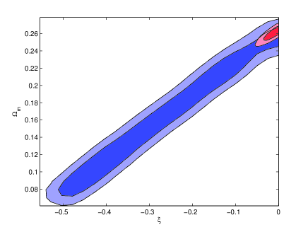
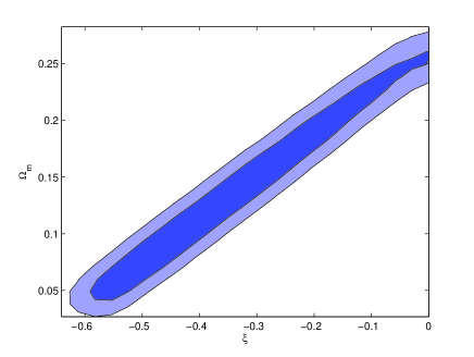
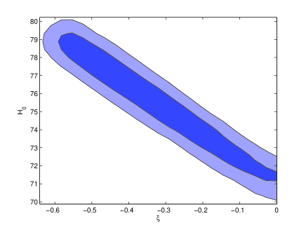
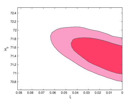
In Table 4 we show the MCMC constraints at $68\%$ c.l. for the coupled universe from Planck data alone and from Planck data combined with Euclid data. For this last case we also fit the data fixing $\xi$ to $0$, thus performing a standard analysis in a universe where dark matter and dark energy are not interacting, in order to show the importance of the degeneracies introduced by the presence of a coupling $\xi$ on the other cosmological parameters errors. There is a very high level of correlation among the dimensionless coupling $\xi$ and the parameters $H_{0}$ and $\Omega_{c}h^{2}$ in the Planck analysis (see also Figs. 3 and 4). When Planck and Euclid data are combined, the degeneracy between $\xi$ and $H_{0}$ is broken, leading to a much better constrain on the coupling parameter $\xi$ than when using CMB data aloneMartinelli:2010rt , as one can notice from Table 4 and Fig. 2. However, the degeneracy between $\xi$ and $\Omega_{c}h^{2}$ is not broken by the combination of Planck and Euclid, thus it will be possible to further improve the constraints on $\xi$ with independent measurements of $\Omega_{c}$. We also note that the constraints on the standard cosmological parameters are in good agreement with those reported in Refregier:2010ss .

	Planck		Planck+Euclid
Model	Varying $\xi$	$\xi=0$	Varying $\xi$	$\xi=0$
Parameter
$\Delta{(\Omega_{b}h^{2})}$	$0.00013$	$0.00013$	$0.00010$	$0.00010$
$\Delta{(\Omega_{c}h^{2})}$	$0.0299$	$0.0010$	$0.0024$	$0.00055$
$\Delta{(\theta_{s})}$	$0.0023$	$0.00026$	$0.00027$	$0.00023$
$\Delta{(\tau)}$	$0.0042$	$0.0042$	$0.0026$	$0.0026$
$\Delta{(n_{s})}$	$0.0030$	$0.0031$	$0.0029$	$0.0027$
$\Delta{(\log[10^{10}A_{s}])}$	$0.013$	$0.013$	$0.0097$	$0.0093$
$\Delta{(H_{0})}$	$2.28$	$0.43$	$0.29$	$0.27$
$\Delta{(\Omega_{\Lambda})}$	$0.0614$	$0.0050$	$0.0062$	$0.0026$
$\xi$	$>-0.56$	$-$	$>-0.05$	$-$

Table 4: $68\%$ c.l. errors on cosmological parameters. Upper limits on $\xi$ are $95\%$ c.l. constraints.

As stated above, future surveys like Euclid will be able to tomographically reconstruct the matter distribution. Exploiting this possibility would improve the constraints, but, as already pointed out in Martinelli:2010wn , the non tomographic analysis can be thought as a conservative estimation of the constraints as we are not including systematic effects.

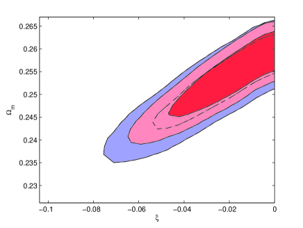
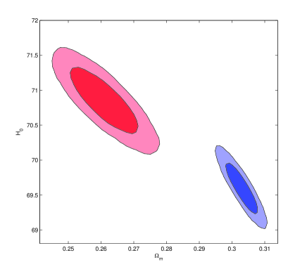
Table 5 contains both the results from the combination of Planck and Euclid data and those from the combination of Planck and LSST. Notice that the results are quite similar. However, the slightly better constraints on $\xi$ from the Planck plus Euclid combination leads to a better measurement of the cold dark matter content of the universe than the one performed by Planck plus LSST data (see also Fig. 1).
Moreover, the difference between Planck+Euclid and Planck+LSST results would be bigger if systematic effects are included, as LSST, being a ground based survey, will be more affected by these.

	Planck+Euclid	Planck+LSST
Parameter
$\Delta{(\Omega_{b}h^{2})}$	$0.00010$	$0.00010$
$\Delta{(\Omega_{c}h^{2})}$	$0.0024$	$0.0026$
$\Delta{(\theta_{s})}$	$0.00027$	$0.00028$
$\Delta{(\tau)}$	$0.0026$	$0.0027$
$\Delta{(n_{s})}$	$0.0029$	$0.0029$
$\Delta{(\log[10^{10}A_{s}])}$	$0.0097$	$0.010$
$\Delta{(H_{0})}$	$0.29$	$0.29$
$\Delta{(\Omega_{\Lambda})}$	$0.0062$	$0.0065$
$\xi$	$>-0.04$	$>-0.06$

Table 5: $68\%$ c.l. errors on cosmological parameters. Upper limits on $\xi$ are $95\%$ c.l. constraints.

Figure 1: 2-D constraints on $\xi$ and $\Omega_{m}$ using Planck and LSST data (blue contours) and Planck and Euclid data (red contours).

In addition, we have also (wrongly) fitted a mock dataset with $\xi=-0.1$ to a non interacting cosmology in which the dimensionless coupling vanishes ($\xi=0$). From this exercise we find a consistent bias in the recovered best fit value of the cosmological parameters due to the strong degeneracies among $\xi$ and both the Hubble constant $H_{0}$ and the matter energy density $\Omega_{m}$ parameters, see Tab.6. 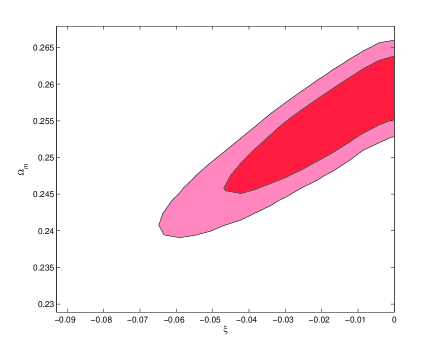Note, from the results depicted in Figs. 3, 4 and 5 and also from the results in Tab. 6 that the shift in the best fit values is, as expected, along the direction of the degeneracy of $\xi$ with these parameters. These results show that even for a small value of $\xi$, the best fit values recovered by wrongly assuming that t here is no dark coupling are more than $68\%$ c.l. (for some parameters at more than $95\%$ c.l.) away from the correct fiducial values, and may induce an underestimation of both $H_{0}$ and $\sigma_{8}$ and an overestimation of $\Omega_{c}h^{2}$. In the last column in Tab. 6 we show the difference between the wrong value estimated fixing $\xi=0$ and the fiducial value, relative to the 1$\sigma$ error: as expected the largest shifts are in the parameters that are directly involved in determining the energy momentum transfer between components, namely matter and dark energy densities and Hubble parameter (see section II). We note that also other parameters, as $\sigma_{8}$ and $n_{s}$, have significant shifts.
We conclude, hence, that future analyses of high precision data from Euclid and Planck need to consider possible deviations from the minimal $\Lambda$CDM scenario in order to avoid biases in the measurements of the cosmological parameters.

	Planck+Euclid		Fiducial values
Model:	$\xi=0$	varying $\xi$
Parameter
$\Omega_{b}h^{2}$	$0.02259\pm 0.00010$	$0.02257\pm 0.00010$	$0.02258$
$\Omega_{c}h^{2}$	$0.1245\pm 0.00061$	$0.1083\pm 0.0024$	$0.1109$
$\tau$	$0.086\pm 0.0029$	$0.090\pm 0.0033$	$0.088$
$n_{s}$	$0.955\pm 0.0014$	$0.961\pm 0.0028$	$0.963$
$H_{0}$	$69.6\pm 0.23$	$70.9\pm 0.30$	$71.0$
$\Omega_{\Lambda}$	$0.697\pm 0.0031$	$0.739\pm 0.0066$	$0.735$
$\sigma_{8}$	$0.752\pm 0.00044$	$0.841\pm 0.019$	$0.82$

Table 6: Best fit values and $68\%$ c.l. errors on cosmological parameters for the case in which a fiducial model with $\xi=-0.1$ is fitted to a $\Lambda$CDM model where $\xi=0$ is assumed.

Figure 2: 2-D constraints on $\xi$ and $\Omega_{m}$ using Planck (blue contours) and Planck plus Euclid (red contours).

Figure 3: Top panel: $68\%$ and $95\%$ c.l. contours in the ($\Omega_{m}$, $\xi$) plane from Planck data only. Bottom panel: same as in the top panel, but for the combination of Planck plus Euclid data (note the different scale for the x-axis).

Figure 4: Top panel: $68\%$ and $95\%$ c.l. contours in the ($H_{0}$, $\xi$) plane from Planck data only. Bottom panel: same as in the top panel, but for the combination of Planck plus Euclid data (note the different scale for the x-axis).

Figure 5: $68\%$ and $95\%$ confidence levels from Planck plus Euclid data when a fiducial cosmology with $\xi=-0.1$ is fitted to a non interacting cosmology with $\xi$ fixed to $0$ (blue countours) or to an interacting cosmology in which $\xi$ is allowed to vary.

VII Conclusions

The current accelerated expansion of the universe is driven by the so-called dark energy. This negative pressure component could be interpreted as the vacuum energy density, or as a cosmic, dynamical scalar field. If a cosmic quintessence field is present in nature, it may couple to the other fields in nature. While the couplings of the quintessence field to ordinary matter are severely constrained, an energy exchange among the dark matter and dark energy sectors is allowed by current observations. Interacting cosmologies, in order to fit Cosmic Microwave Background observations, predict non standard values for the low redshift universe observables. Therefore, measurements of the growth of structure and of the dark matter distribution via galaxy and weak lensing surveys offer a unique window to study the nature of the dark sectors.

The major goals of the on-going Planck experiment and the next generation of galaxy surveys are to determine the nature of the dark energy component and to measure the remaining cosmological parameters with unprecedented precision. In this study we have exploited the capabilities of the former experiments to improve current constraints on the dimensionless coupling $\xi$, which drives the energy flow between the dark energy and dark matter sectors Gavela:2009cy .

We have generated mock data for both the Planck experiment and the Euclid and LSST-like weak lensing surveys. CMB gravitational lensing extraction has also been included in the analysis. For the weak lensing surveys, the observable we have exploited here is the convergence power spectrum. The mock data have then been analyzed using MCMC techniques to compute the errors on the several cosmological parameters considered here. The constraints on the dimensionless coupling parameter of the interacting model fully explored here, $\xi$, are greatly improved with respect to previous analyses in which only CMB probes were considered. We find $\xi>-0.04$ at the $95\%$ c.l. for the combination of Planck survey and Euclid weak lensing data. Data from a LSST-like survey combined with data from the Planck experiment could also provide a lower bound on $\xi$ of $-0.06$ at the $95\%$ c.l.. The coupling parameter $\xi$ is strongly degenerate with the cold dark matter density $\Omega_{c}h^{2}$ and the Hubble constant $H_{0}$. These degeneracies may cause important biases in the cosmological parameter values if in the universe there exists an interaction among the dark sectors. Future experiments may therefore include also coupled cosmologies as possible scenarios when fitting their data. Finally we conclude noting that, as recently outlined by Tarrant:2011qe , coupled quintessence is expected to have a distinctive impact on the formation of structures at galaxy clusters scales. In our work we limited our analysis to linear scales, but for the analysis of real future data, it will be necessary a precise modeling of the effects of coupled quintessence on non-linear scales. At the same time, this small scale effect will offer a way to constrain coupled cosmologies through measurements of the galaxy clusters mass distribution.

VIII Acknowledgments

We thank Alan Heavens for very useful comments. This work is supported by PRIN-INAF, ”Astronomy probes fundamental physics”. Support was given by the Italian Space Agency through the ASI contracts Euclid- IC (I/031/10/0). The work of O.M. is supported by a MICINN Ramón y Cajal contract, by AYA2008-03531 and the Consolider Ingenio-2010 project CSD2007-00060.

References

- (1) E. Komatsu et al. [WMAP Collaboration], Astrophys. J. Suppl. 192, 18 (2011) [arXiv:1001.4538 [astro-ph.CO]] ; D. Larson et al., Astrophys. J. Suppl. 192, 16 (2011) [arXiv:1001.4635 [astro-ph.CO]].
- (2) B. A. Reid et al. [SDSS Collaboration], Mon. Not. Roy. Astron. Soc. 401, 2148 (2010) [arXiv:0907.1660 [astro-ph.CO]] ; B. A. Reid et al., Mon. Not. Roy. Astron. Soc. 404, 60 (2010) [arXiv:0907.1659 [astro-ph.CO]].
- (3) R. Amanullah et al., Astrophys. J. 716, 712 (2010) [arXiv:1004.1711 [astro-ph.CO]].
- (4) S. M. Carroll, Phys. Rev. Lett. 81, 3067 (1998) [arXiv:astro-ph/9806099].
- (5) L. Amendola, Phys. Rev. D 62, 043511 (2000) [arXiv:astro-ph/9908023].
- (6) L. Amendola, Mon. Not. Roy. Astron. Soc. 312, 521 (2000) [arXiv:astro-ph/9906073].
- (7) L. Amendola, Phys. Rev. D 60, 043501 (1999) [arXiv:astro-ph/9904120].
- (8) L. Amendola and D. Tocchini-Valentini, Phys. Rev. D 64, 043509 (2001) [arXiv:astro-ph/0011243].
- (9) L. Amendola, Phys. Rev. D 69, 103524 (2004) [arXiv:astro-ph/0311175].
- (10) L. Amendola, G. Camargo Campos and R. Rosenfeld, Phys. Rev. D 75 (2007) 083506 [arXiv:astro-ph/0610806].
- (11) J. Valiviita, E. Majerotto and R. Maartens, JCAP 0807, 020 (2008) [arXiv:0804.0232 [astro-ph]].
- (12) J. H. He, B. Wang and E. Abdalla, Phys. Lett. B 671, 139 (2009) [arXiv:0807.3471 [gr-qc]].
- (13) B. M. Jackson, A. Taylor and A. Berera, Phys. Rev. D 79, 043526 (2009) [arXiv:0901.3272 [astro-ph.CO]].
- (14) M. B. Gavela, D. Hernandez, L. L. Honorez, O. Mena and S. Rigolin, JCAP 0907, 034 (2009) [Erratum-ibid. 1005, E01 (2010)] [arXiv:0901.1611 [astro-ph]].
- (15) G. Caldera-Cabral, R. Maartens and B. M. Schaefer, JCAP 0907, 027 (2009) [arXiv:0905.0492 [astro-ph.CO]].
- (16) J. Valiviita, R. Maartens and E. Majerotto, Mon. Not. Roy. Astron. Soc. 402, 2355 (2010) [arXiv:0907.4987 [astro-ph.CO]].
- (17) E. Majerotto, J. Valiviita and R. Maartens, Mon. Not. Roy. Astron. Soc. 402, 2344 (2010) [arXiv:0907.4981 [astro-ph.CO]].
- (18) M. B. Gavela, L. Lopez Honorez, O. Mena and S. Rigolin, JCAP 1011, 044 (2010) [arXiv:1005.0295 [astro-ph.CO]].
- (19) L. L. Honorez, B. A. Reid, O. Mena, L. Verde and R. Jimenez, JCAP 1009, 029 (2010) [arXiv:1006.0877 [astro-ph.CO]].
- (20) M. Martinelli, L. Lopez Honorez, A. Melchiorri and O. Mena, Phys. Rev. D 81, 103534 (2010) [arXiv:1004.2410 [astro-ph.CO]].
- (21) L. Lopez Honorez, O. Mena and G. Panotopoulos, Phys. Rev. D 82, 123525 (2010) [arXiv:1009.5263 [astro-ph.CO]].
- (22) A. Refregier et al., arXiv:astro-ph/0610062.
- (23) A. Refregier, A. Amara, T. D. Kitching, A. Rassat, R. Scaramella, J. Weller and f. t. E. Consortium, arXiv:1001.0061 [astro-ph.IM].
- (24) [LSST Science Collaborations and LSST Project Collaboration], arXiv:0912.0201 [astro-ph.IM].
- (25) H. Kodama, M. Sasaki, Prog. Theor. Phys. Suppl. 78, 1-166 (1984).
- (26) S. Chongchitnan, Phys. Rev. D79, 043522 (2009). [arXiv:0810.5411 [astro-ph]].
- (27) P. S. Corasaniti, Phys. Rev. D78, 083538 (2008). [arXiv:0808.1646 [astro-ph]].
- (28) A. Lewis, A. Challinor and A. Lasenby, Astrophys. J. 538 (2000) 473.
- (29) M. Bartelmann and P. Schneider, Phys. Rept. 340 (2001) 291 [arXiv:astro-ph/9912508].
- (30) D. Huterer, Gen. Rel. Grav. 42 (2010) 2177 [arXiv:1001.1758 [astro-ph.CO]].
- (31) P. Schneider, L. van Waerbeke, M. Kilbinger and Y. Mellier, Astron. Astrophys. 396 (2002) 1 [arXiv:astro-ph/0206182].
- (32) L. Perotto, J. Lesgourgues, S. Hannestad, H. Tu and Y. Y. Y. Wong, JCAP 0610 (2006) 013 [arXiv:astro-ph/0606227].
- (33) E. Calabrese, A. Cooray, M. Martinelli, A. Melchiorri, L. Pagano, A. Slosar and G. F. Smoot, Phys. Rev. D 80 (2009) 103516 [arXiv:0908.1585 [astro-ph.CO]].
- (34) C. M. Hirata and U. Seljak, Phys. Rev. D 68 (2003) 083002 [arXiv:astro-ph/0306354].
- (35) T. Okamoto and W. Hu, Phys. Rev. D 67 (2003) 083002 [arXiv:astro-ph/0301031].
- (36) A. F. Heavens, 2003, MNRAS, 323, 1327
- (37) P. G. Castro, A. F. Heavens, T. D. Kitching, 2005, Phys. Rev. D, 72, 3516
- (38) A. F. Heavens, T. D. Kitching, A. N. Taylor, 2006, MNRAS, 373, 105
- (39) T. D. Kitching, A. F. Heavens, A. N. Taylor, M. L. Brown, K. Meisenheimer, C. Wolf, M. E. Gray, D. J. Bacon, 2007, MNRAS, 376, 771
- (40) S. Hannestad, H. Tu and Y. Y. Y. Wong, JCAP 0606 (2006) 025 [arXiv:astro-ph/0603019].
- (41) Bacon, D.; et al.; 2003; MNRAS, 363, 723-733
- (42) Massey R.; et al.; 2007, ApJS, 172, 239
- (43) Taylor, A. N.; et al.; 2004, MNRAS, 353, 1176
- (44) A. R. Cooray, Astron. Astrophys. 348 (1999) 31 [arXiv:astro-ph/9904246].
- (45) R. E. Smith et al. [The Virgo Consortium Collaboration], Mon. Not. Roy. Astron. Soc. 341 (2003) 1311 [arXiv:astro-ph/0207664].
- (46) F. B. Abdalla, A. Amara, P. Capak, E. S. Cypriano, O. Lahav and J. Rhodes, Mon. Not. Roy. Astron. Soc. 387 (2008) 969 [arXiv:0705.1437 [astro-ph]].
- (47) L. Fu et al., Astron. Astrophys. 479 (2008) 9 [arXiv:0712.0884 [astro-ph]].
- (48) [Planck Collaboration], arXiv:astro-ph/0604069.
- (49) A. Lewis and S. Bridle, Phys. Rev. D 66, 103511 (2002) (Available from http://cosmologist.info.)
- (50) M. Martinelli, E. Calabrese, F. De Bernardis, A. Melchiorri, L. Pagano and R. Scaramella, Phys. Rev. D 83 (2011) 023012 [arXiv:1010.5755 [astro-ph.CO]].
- (51) E. R. M. Tarrant, C. van de Bruck, E. J. Copeland and A. M. Green, arXiv:1103.0694 [astro-ph.CO].