Lattice QCD study of mixed systems of pions and kaons
Abstract
The different ground state energies of -pion and -kaon systems for are studied in lattice QCD. These energies are then used to extract the various two- and three- body interactions that occur in these systems. Particular attention is paid to additional thermal states present in the spectrum because of the finite temporal extent. These calculations are performed using one ensemble of 2+1 flavor anisotropic lattices with a spatial lattice spacing fm, an anisotropy factor , and a spatial volume . The quark masses used correspond to pion and kaon masses of and , respectively. The isospin and strangeness chemical potentials of these systems are found to be in the region where chiral perturbation theory and hadronic models predict a phase transition between a pion condensed phase and a kaon condensed phase.
I Introduction
An important goal of nuclear physics is to calculate nuclear properties and processes from Quantum Chromodynamics (QCD). The only known way to perform such calculations in an ab initio manner is using the non-perturbative formulation of QCD on a space-time lattice (lattice QCD). Much progress has been made in recent years in studying few hadrons systems, see for example the recent review of Ref. Beane et al. (2010). Many channels of meson-meson, meson-baryon and baryon-baryon interactions have been studied using the finite volume behavior of two-particle energy levels Hamber et al. (1983); Lüscher (1986a, b, 1991). Ground state energies of three- Beane et al. (2009a) and four- Yamazaki et al. (2010) baryon systems have been computed for the first time in QCD and quenched QCD, respectively. To become a central part of nuclear physics, the successes of lattice QCD in the realm of few-hadron systems must be translated into the realm of many hadrons and the complexity frontier must be addressed. To this end, recent work has focused on numerical investigations in systems of up to twelve pions or kaons Beane et al. (2008a); Detmold et al. (2008a); Detmold et al. (2008b); Detmold (2008), and algorithms Detmold and Savage (2010) have been constructed to greatly extend these studies. An important outcome of these studies was the extraction of the two- and three- body interactions in pion and, separately, kaon systems. The shifts in the -meson energy levels at finite volume were calculated numerically and then compared with the analytical expectations derived in Refs. Beane et al. (2007); Tan (2008); Detmold and Savage (2008). These calculations also probed the relation between isospin(hypercharge) chemical potential and isospin(hypercharge) density, finding agreement with the predictions of chiral perturbation theory Son and Stephanov (2001a); Kogut and Toublan (2001).
In this work, we study more complicated multi-meson systems involving both pions and kaons. As in the single species case, the expected volume dependence of the energy of an -, - system has been computed Smigielski and Wasem (2009) and these calculations will enable us to extract the scattering lengths for the three two-body interactions, , , , and also to study the various zero momentum three-body interactions, parameterized as , , , (restricted to the maximal isospin in each case). Multi-meson systems such as these exhibit a rich phase structure Dashen and Manassah (1974); Son and Stephanov (2001a) and are phenomenologically relevant in a number of settings ranging from RHIC Klein et al. (2003) to the interiors of neutron stars Kaplan and Nelson (1986). At low temperatures, the ground-state of a finite density system of, for example, pions is expected to undergo a transition from a Bose-Einstein condensed phase Sawyer (1972); Scalapino (1972); Baym (1973); Dashen and Manassah (1974); Campbell et al. (1975a, b) to a BCS-type superconducting phase as the isospin chemical potential is increased, and other interesting phenomena such as -condensation may also occur Voskresensky (1997); Sannino (2003); Aharony et al. (2008). Similar effects are expected in kaon systems. The phase structure of a mixed system of pions and kaons is a less well investigated question. Studies in the NJL (Nambu–Jona-Lasinio) model, Barducci et al. (2005); He et al. (2005); Warringa et al. (2005), random matrix theory Arai and Yoshinaga (2009), and SU(3) chiral perturbation theory (PT) with non-zero isospin and hypercharge chemical potentials Kogut and Toublan (2001), suggest that pion and kaon condensed phases compete in interesting ways for different ranges of isospin and hypercharge chemical potentials.
In the following, we focus on numerical analysis of lattice QCD realizations of these complex multi-meson systems and on the methodology needed to extract the two- and three-body interactions. We calculate the 90 possible two-point correlation functions involving -s and -s for all . These results are then analyzed to extract the ground state energies of the appropriate quantum numbers, taking care to account for thermal excitations in the lattice volume. Finally, the resulting large set of energies is used to extract the seven underlying interactions discussed above. The extracted energies also allow us to study the chemical potential of these systems. This study is performed using a single ensemble of 2+1 flavor anisotropic gauge field configurations generated by the Hadron Spectrum Collaboration Lin et al. (2009) and so should be viewed as an exploratory study, testing methods necessary for analysis of complicated many body systems. Future work with different lattice spacings, volumes and quark masses will allow contact with experiment Pislak et al. (2001, 2003); Adeva et al. (2005); Batley et al. (2006); Adeva et al. (2000), in the case of two-body interactions, and with other lattice studies.
II Multi-hadron correlation functions
In order to extract the energies of the multi meson systems, we will study the behavior of two point correlation functions
| (1) |
where the pion and kaon interpolating operators are defined in terms of quark fields as and , respectively. This system corresponds to a system of ’s and ’s with total momentum, .
It is instructive to first consider the form of such correlation functions which can be generically expressed as
| (2) |
for some interpolating operators, , with commensurate quantum numbers.111The creation and annihilation interpolating operators are not in general Hermitian conjugates of one another. In a system with infinite (Euclidean) temporal extent, application of the transfer matrix formalism shows that
| (3) |
where the sum runs over all eigenstates with the quantum numbers of the operators under study. The are the energies of eigenstates and . At large Euclidean time, the correlator is dominated by the ground state energy of the system, . However, in a system with a finite temporal extent, , a natural choice of temporal boundary conditions for quark and gluon fields, anti-periodic and periodic respectively, will force to be periodic (assuming the operators under study are bosonic, as in Eq. (1)). The expected form of the correlation function can again be inferred:
| (4) |
with . The contributions on the right-hand side of Eq. (4) can be separated into two distinct classes. The first class is defined by choosing to be the vacuum state () and correspond to the ground state and excited states of the system. These contributions are special as they persist in the (or zero temperature) limit. The remaining contributions exist solely due to the finite time extent and are known as thermal states Beane et al. (2008a); Detmold et al. (2008b); Beane et al. (2009b); Richards (2001); Gockeler et al. (2002); Prelovsek and Mohler (2009); Detmold et al. (2009). These states vanish as because of the first exponential under the sum in Eq. (4).
Thermal contributions can be illustrated with a concrete example. Consider which corresponds to a system with the quantum numbers of four pions. The correlation function is dominated by a sum of three contributions in the large limit:
| (5) |
where , the ellipsis denotes contributions involving excited pion systems that we will ignore in the current discussion, and the ’s are constant with respect to time. The first term in Eq. (II) corresponds to states where all four ’s propagate forward in time () and four ’s propagate backward in time (). The second term represents three ’s propagating forward in time and one propagating backward in time () as well as three ’s propagating backward in time and one propagating forward in time (). Finally, the last term arises from two ’s propagating forward in time and two ’s propagating backward in time ().
The general form for the correlation function of -pions and -kaons can be straightforwardly worked out and is given by the following
| (6) |
where , the ellipsis denotes excited state contributions, and the last term in Eq. (6) is only present when are even. It is apparent that the number of possible terms contributing to grows with and . Locality of the transfer matrix guarantees that the eigen-energies appearing in many places in different are identical. Consequently, multiple correlation functions (choices of and ) can be used to extract the common set of eigen-energies.
Thermal states contribute to most lattice calculations and need to be considered in precise analyses. They are particularly prevalent in the multi-hadron context as these systems easily factorize into multiple color singlet states that can propagate over long distances. In Refs. Beane et al. (2008a); Detmold et al. (2008a); Detmold et al. (2008b), the issue of thermal states was avoided by using Dirichlet boundary conditions. In principle, such boundary conditions introduce unknown contamination into correlation functions, however these works analyzed correlations significantly separated from the boundary to reduce such effects.
III Details of Lattice Calculation
The lattice calculations presented in this work are based on a single ensemble of anisotropic gauge field configurations generated by the Hadron Spectrum Collaboration Lin et al. (2009). These configurations were generated using a stout smeared Morningstar and Peardon (2004) gauge action and a 2+1 flavor clover fermion action; further details can be found in Refs. Lin et al. (2009). The spatial and temporal lattice spacings are and respectively, where is the renormalized anisotropy. The lattices have a volume of , corresponding in physical units to , and the light and strange quark masses are such that the pion and kaon have masses of and . These configurations have been extensively studied by the HSC and NPLQCD collaborations. For this study, an ensemble of 400 configurations were chosen from a long stream of 10,000 trajectories and are well separated in Monte-Carlo time such that autocorrelations are reduced.
Our analysis makes use of light and strange quark propagators generated by the NPLQCD collaboration. For each configuration, randomly positioned APE Best et al. (1997); Güsken et al. (1989) smeared sources were used to generate approximately 75 propagators. The EigCG inverter Stathopoulos and Orginos (2010) was used to perform the multiple inversions efficiently. These propagators were then APE smeared at the sink and combined into the correlation functions of Eq. (1).
Naively, the number of contractions involved in the correlation functions of Eq. (1) is enormous, . To compute the requisite contractions, we extend the methods developed in Ref. Detmold et al. (2008a) to the mixed species case. Following the manipulations of Ref. Detmold et al. (2008a) it is straightforward to show that for arbitrary matrices, :
| (7) |
with
| (8) | |||||
| (9) |
where the correspond to the source and sink smeared quark propagators of flavor . Additionally, one can generalize the results of the single species case to show that in the mixed species case,
| (10) |
where
| (11) |
By expanding the exponential to a particular order in and , and equating Eq. (III) and Eq. (10), one can identify the function .
The computational complexity of these two-species contractions is significantly more than that of the single species cases studied previously. The reader can find an example, the correlator, in Eq. (37). As in the single species cases Detmold et al. (2008a); Detmold et al. (2008b), high precision arithmetic is required to perform these contractions correctly and this is implemented using the arprec and qd libraries Bailey et al. (2002). Explicit calculations for all correlation functions show these correlators vanish to the requisite precision and are an effective check of the correctness of our code. The computational cost of computing all contractions for and all is approximately twenty minutes on a single core, compared to a few seconds for the single species case. While not available at the time that the current calculations began, the recursive constructions developed in Ref. Detmold and Savage (2010) provide an alternate, and computationally more efficient, way of generating the contractions. The results of both methods agree to arbitrary precision.222In future calculations that extend the number of pions and kaons beyond twelve, these recursive techniques will be critical as the explicit code generated for all the requisite contractions would be unmanageably large.
IV Volume Dependence of Multi-hadron energies
As discussed above, the calculations of the correlators in Eq. (6) determine the energies of the mesonic systems. These can in turn be used to determine the interactions through the well-known results of Lüscher Lüscher (1986a, b) in the two body case and the results of Refs. Beane et al. (2007); Tan (2008); Detmold and Savage (2008); Smigielski and Wasem (2009) in the many meson case where a perturbative expansion in the inverse volume is performed.
IV.1 Volume dependence of two particle energies
An extraction of the scattering lengths from the single species and mixed species two particle systems provides a baseline reference with which to compare the results of the multi-particle analysis. In the center-of-mass frame, we define the interaction momentum, , from the energy shift . is determined from lattice calculations and one first solves for the momentum Lüscher (1986b). Lüscher’s formula relates this momentum to the phase-shift, , of two particle scattering as
| (12) |
where and
| (13) |
is a regulated three dimensional zeta function. By expanding the left-hand side of Eq. (12) using the effective-range expansion, , the scattering length, , can be determined. In the absence of interactions, possesses poles at for . With interactions these poles are shifted. One then computes as:
| (14) |
Using this formula with the associated one-body and two-body energies will yield precise determinations of the scattering lengths as the one- and two- body energies are the most cleanly determined and the above results only omit exponentially suppressed finite volume effects.
IV.2 Volume dependence of multi-meson energies
In Ref. Smigielski and Wasem (2009), the energy shift of a system -pions and -kaons in a finite volume from the corresponding non-interacting system was calculated. The shift is given by:
| (15) |
with and and
| (18) | ||||
| (21) |
| (22) |
where the parameters are related to the scattering lengths and effective ranges through Detmold et al. (2008a); Smigielski and Wasem (2009):
| (23) |
It is the parameters that will be determined in the current lattice calculations. The four volume dependent (but renormalization scale independent) quantities characterizing the momentum independent three-body interactions are defined by ():
| (24) |
and
| (25) |
with . The functions , , , and along with the coefficients are defined in Ref. Smigielski and Wasem (2009). The finite parts of and are scheme dependent quantities where changes in the value will be compensated by changes in ; the numerical values for the Minimal Subtraction (MS) scheme are given in Ref. Smigielski and Wasem (2009). However, the are scheme independent and these are the quantities that will be determined during a lattice calculation. Furthermore, the three-body interactions in the and cases depend on the mass ratio, . Finally, in the limit of or , this result simplifies to the previously determined -boson case while the limit with and all interactions set to be equal it simplifies to the -boson case.
V Analysis Strategies
After calculating the above correlation functions on the ensemble of gauge configurations, we obtain lattice measurements of in Eq. (1). Provided that we can reliably deal with the presence of thermal and excited states, these allow us to extract the ground state energies of the -pion, -kaon systems. By matching these measurements onto the analytic expectations of Eq. (IV.2), the various two- and three-body interaction parameters can then be extracted. There are many ways in which such an analysis could proceed. One could attempt to directly fit the correlation functions in terms of overlap factors, and the scattering parameters and three-body interactions by inserting the explicit form of the energies from Eq. (IV.2). However, we choose to perform this as a two stage analysis, first extracting the various energies by fits to the correlation functions using the model functions of Eq. (6) and then subsequently fitting these energies to the analytic forms of Eq. (IV.2) to extract the interaction parameters. The primary advantage of this approach to performing the fits is increased stability, however, care must be taken to preserve the significant correlations between the different correlation functions which are computed on the same set of gauge configurations.
V.1 Wavefunction Overlap
As shown in Eq. (6), the -factors for each term are in general distinct. This makes for a difficult analysis since there are large numbers of linear and non-linear fit parameters that must be determined. In the non-interacting system, these -factors are simply related. In the single-species case, the relation would be such that is common to each term. The factorial simply counts the number of ways that -pions propagate forward and propagate backward. Generalizing this to the multi-meson case leads to . In an interacting system, however, this relationship does not hold. Nevertheless, in this work, we study pion and kaon systems with relatively weak interactions, and therefore we employ the ansatz above for the wavefunction factors. We stress this is a crucial assumption, allowing us to subsequently fit all 90 correlators. As a check, analyses were also performed allowing the -factors to remain distinct for as many correlators as possible. Results from both methods were found to agree within uncertainty, but a full analysis using independent ’s proved unfeasible.
An alternative method that can be utilized for these systems is the method of Variable Projection (VARPRO) Kaufman (1975); Fleming (2004) which eliminates linear fit parameters by performing their minimization analytically. This approach is useful in the case of unrelated ’s from Eq. (4). Additionally, when many energies exist to be fitted, convergence to the minimum of parameter space is not always guaranteed, particularly if the minimum is flat. To aid convergence, Bayesian priors Lepage et al. (2002); Howson and Urbach (2005) can be implemented so the physically reasonable region of parameter space is immediately tested. In an earlier stage of our analysis, the VARPRO method (with priors) was used for correlators with lower total particle number. The results were found to agree within uncertainty with the results using the ansatz above.
As a final check, the fitted energies were substituted back into the form for the correlator and compared against the original data set. Consistency was achieved within uncertainty. Therefore, for the remainder of this work, we assume the simplified form for the wavefunction overlap.
V.2 Thermal effects of Correlation Functions
A particular multi-meson correlator depends not only on its ground state energy in the large- limit, but also upon fewer body energies in the thermal states that were discussed earlier. To account for this, we began by fitting the one pion(kaon) correlator to determine () with a bootstrap method as will be explained below. Once these values were known, we turned to the two pion(kaon) correlator. This correlator depends on () and (). Instead of refitting both energies, we used previous bootstrapped values of () in the two pion(kaon) fit function. This is reasonable since the cleanest signal for the energy will come from its respective correlator. To preserve all covariances in the data, the same bootstrap sample of gauge field configurations was used for all correlators. This sequential procedure was used to build up the analysis and ascertain all of the multi-meson energies. The fitted results for the energies and their statistical and systematic errors can be found in Tables 1 and LABEL:multiSpeciesEnergyTable.
V.3 Statistical Analysis
The correlation functions span the time interval and a suitable subinterval, where the fit formula is applicable, must be chosen. As a first step, the (periodic) correlation function data was reflected around its midpoint in order to improve statistics. Effective mass plots for all correlation functions were constructed, allowing initial estimates to be made of where (in time) contamination from excited states ceases. These plots revealed that excited state contributions are suppressed by . Therefore, in an effort to be as general as possible, fits were run on all time intervals, , such that and . Using intervals beyond these values showed no improvement in fit results.
In this work, we utilized the bootstrap method of statistical resampling to estimate uncertainties. To construct the bootstrap ensembles, we first averaged over correlators from all sources on each gauge configurations, for each . Let be a given correlation function for some fixed number of pions and kaons, and , calculated on a given gauge field configuration at time . Then we denote this set as , with . The data covariance matrix is defined from the full data set as:
| (26) |
where .
Next, we randomly sampled configurations from the full data set and constructed a bootstrap sample, of elements, for each time . This sample was averaged to yield and this entire process repeated times where , resulting in: . For each of the , a function was determined as:
| (27) |
where represents the fit model in Eq. (6). Each of the functions were minimized and results recorded.
In order to assess the reliability of the fits, we define the goodness-of-fit, , where is the number of degrees-of-freedom, for each . Once a best fit energy is selected on each bootstrap sample, we determine a weighted average for the ensemble,
| (28) |
with weights , and a weighted standard deviation,
| (29) |
Above, and .
To assign a systematic uncertainty for the extracted energies, we return to the fits performed to the correlators. This is a necessary component of the analysis since there exists arbitrariness in the choice of which and which were selected for the correlation function fits as explained above. The systematic error on the best fit energy is defined as
| (30) |
where are the energies extracted from using the time intervals and .
V.4 Two and Three Body Parameters
The second stage of our analysis now focuses on the extraction of the scattering lengths and three-body coefficients from the measured energies using Eqs. (18) and (IV.2). These determinations rely on a second bootstrap analysis involving a resampling of the extracted energies. The bootstrapping procedure for a specific correlation function yielded energies, and these formed the bootstrap samples for the extraction of the two and three-body parameters.
Once the best fit multi-meson energies were known, a very similar procedure used for the analysis of the correlators was used to find the ’s and ’s. Since a bootstrap ensemble exists for every best fit energy value, we created an energy sample, such that . This sample carries an additional vector index that labels the energies within the vector. In the case of single species pion energies (the kaon case is identical), an energy vector initially composed of was used to fit to and . We included another energy and refitted the interaction parameters and repeated this until all the energies were exhausted. In the multi-species case, a base set of along with ten randomly selected multi-species energies was created and fits performed for all seven hadronic parameters. This first set thus made use of 34 different energies. This set was enlarged by one, the parameters were refitted, and the process repeated until all ninety energies were used. The energy covariance matrix used in these fits, is defined according to:
| (31) |
such that , and the energy on each bootstrap is defined as:
| (32) |
where is shorthand notation for the fit functions in Eqs. (IV.2)-(IV.2).
The systematic errors assigned to the ’s and ’s are more complicated than those of the energies. Given a particular energy set of energies that are used to make a determination of ’s and ’s there are different combinations of the intervals that must be fit in order to completely propagate the systematic uncertainties of the energies to those of the interaction parameters (it is because there is a for each best fit energy as well as its systematic counterparts corresponding to the shifted time interval in the forward and backward direction). Even in the single species case, when , there are already combinations. For the multi-species case, it is too costly to fit all these permutations. Rather, we only fit randomly chosen permutations and take the difference of the mean of this set from the best fit and as the systematic error. From fitting all permutations in the single species case, up to , it was seen the systematic error stabilized well before the total number of combinations was computed and we assume this is also the case for the two-species case.
VI Results
VI.1 Energies
Using the methods discussed above, we extracted the energies of the mixed and pure species system, from all ninety correlators. The final extracted values are shown in Tables 1 and LABEL:multiSpeciesEnergyTable below, along with their associated fit ranges. These energies are shown in a three-dimensional plot along with their respective uncertainties in Fig. 1.
The fits become progressively more difficult as the number of mesons grows because of the increasing thermal contamination. This is directly reflected in the quality of the fits decreasing for large meson number in both the pure species and mixed species case. Fits to example correlators are shown in Fig. 2.
VI.2 Interactions
The extractions of interaction parameters from mixed meson energies were performed to yield the three scattering lengths and four three-body coefficients. This work builds upon the studies of Beane et al. (2008a); Detmold et al. (2008a); Detmold et al. (2008b) and presents the first measurements of , and since these parameters can only be measured within the framework of the mixed-meson system.
The most straightforward determination of the scattering lengths is given by using the eigenvalue relation from Eq. (12). Using this, we find,
| (33) |
The three-body coefficients can only be determined within the framework of Eqs. (IV.2), (18), and (IV.2). We also use this same analysis to provide a check on the above results. Given that our analysis provides multiple determinations of the interactions parameters for varying numbers of combinations of energies used in the fits, these must be combined in some way to obtain the final values. Since each separate extraction can be viewed as a somewhat independent measurement, the final value given is taken to be the mean from the set of all extractions. The final uncertainties on the extractions are combinations of statistical uncertainties, systematic uncertainties obtained from variation of the fitting windows as discussed in Sec. V.4, and a second systematic uncertainty determined from the standard deviation of the full set of extractions, combined in quadrature. The systematics are the largest source of uncertainties in the results. The individual extractions of the various parameters and the final extractions are shown in Figs. 3-7. The error bars shown combine the statistical, and systematic uncertainties as discussed in Sec. V in quadrature. The shaded regions with thin borders denote the final results and their uncertainties. For the mixed species extractions, the second shaded band with thick borders, denotes the range of uncertainty in the quoted values from the single species analysis. These are shown together so the reader can see the overlap region between both sets of results. The poorest behavior originates from where the mixed species results drift away from the pure species one. The final values of the interaction parameters for the single-species case are:
| (34) |
whereas for the multi-species case we find:
| (35) |
For the two-body parameters, the perturbative analysis (for both pure species and mixed species) is in agreement with the nonperturbative values. In the above results, only the final uncertainty, including all statistical and systematic contributions, is given as discussed above. A full list of our extractions can be found in Table LABEL:paramValues.
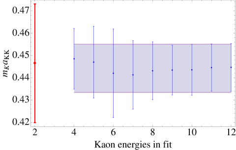
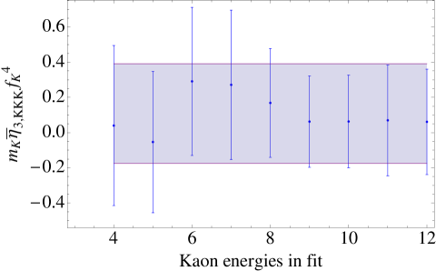
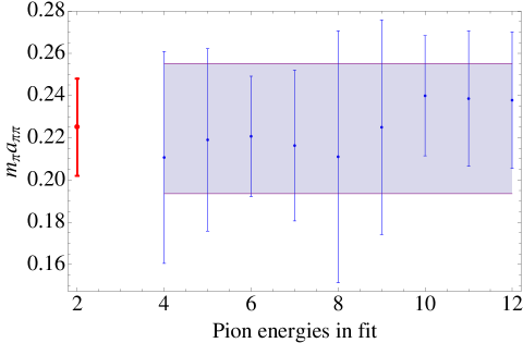
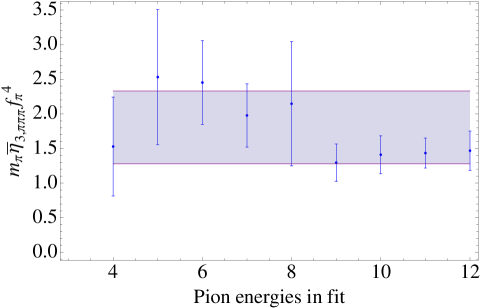
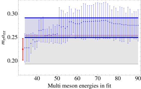
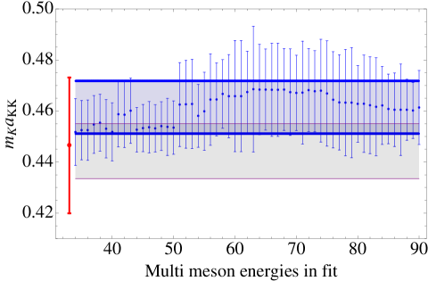
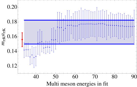
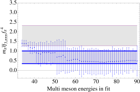
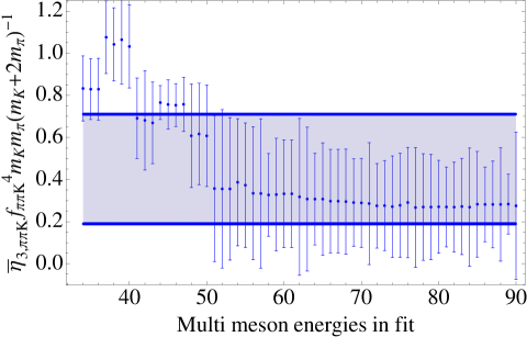
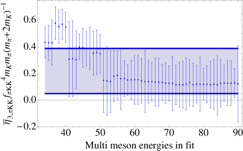
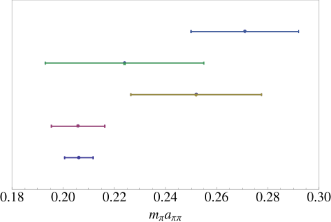
In previous studies, NPLQCD Beane et al. (2006a), CP-PACS Yamazaki et al. (2004), and ETMC Feng et al. (2010) have measured the pion scattering lengths in the isospin, channel. The NPLQCD determination of the scattering length at , yielded whereas an analysis from multi-pion correlators Beane et al. (2008a); Detmold et al. (2008a) yielded an extraction of and (in these results, the first uncertainty is statistical and the other uncertainties are systematics as discussed in the original references. In the ETMC analysis of scattering, is measured at . Fig. 8 shows the dimensionless combination from the current work in comparison to the determinations by other groups at a similar pion mass. However, these results are at non-zero lattice spacing and correspond to different discretizations, so agreement is not necessary. The , scattering length was also determined by the NPLQCD collaboration in Ref. Beane et al. (2008b). An analysis of the two-point kaon correlator yielded a value of , again at MeV. Analysis of multi-kaon correlators Detmold et al. (2008b), led to and where the uncertainties are statistical and systematic respectively. The scattering length has been investigated in quenched Miao et al. (2004) and full QCD Beane et al. (2006b) and the unquenched determination at MeV is . Hence, it is clear the current results are generally consistent with other groups’ extractions. The mixed species three-body parameters are novel results and are found to be of natural size and positive.
VI.3 Isospin and Hypercharge Chemical Potentials
As we have determined the dependence of the energy of the mixed meson systems on the number of pions and kaons, we can construct the isospin and hypercharge (or strangeness) chemical potentials using finite differences following Refs. Detmold et al. (2008b); Detmold et al. (2008a) where systems of pions and kaons were investigated separately. In Refs. Detmold et al. (2008b); Detmold et al. (2008a), remarkable agreement was found between the numerical results and the leading order (LO) PT prediction Son and Stephanov (2001b) of the relation between the isospin(hypercharge) density and chemical potential
| (36) |
with . The situation here is more complicated since there are finite differences acting in various non-orthogonal directions; the differences between and determine while linear combinations of , and determine 333 with and . One goal of this analysis is to see where on the vs. phase diagram Kogut and Toublan (2001), the states created in the lattice calculation lie.
In Ref. Kogut and Toublan (2001), leading order SU(3) PT is used to predict three distinct phases for nonzero isospin and hypercharge chemical potential. The first is the normal phase where the ground state has a net particle number of zero. The other two phases are the pion-condensed and kaon-condensed phases. The transition between the kaon-condensed phase and the pion-condensed phase is predicted to be a first order phase transition, separated by the line , while the transition from the normal phase to either condensed phase is expected to be of second order 444An AdS/QCD based model Albrecht and Erlich (2010) finds these transitions to be of first order. and are defined by the lines and . These predictions assume zero temperature and are likely softened by the non-zero temperature at which the lattice calculation is performed Loewe and Villavicencio (2003).
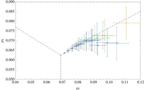
In Fig. 9, both the lattice calculations of and the PT phase boundaries are shown (dashed lines). Data points corresponding to higher numbers of particle states are shown in a orange/reddish color, while lower numbers are given in a blueish/greenish color. Points with large uncertainties are excluded from this figure for clarity (the omitted data correspond to the highest particle numbers). It is striking that the calculated chemical potentials mostly lie near the first-order phase transition line predicted by PT. Further calculations with larger numbers of pions and kaons will be enlightening, but more complex probes of these systems may be needed to fully understand the states that have been produced.
VII Conclusions
In this work, we have numerically studied complex systems of mesons of two distinct flavors, like-charged pions and kaons, and used them to extract information about the two- and three- body interactions amongst pions and kaons. Where known, the interactions were found to be consistent with previous calculations, however, two mixed-species three-body interactions were determined for the first time. Additionally, the isospin and strangeness chemical potentials and phase structure of the system have been investigated, with the systems preferring to probe a region in the plane where PT predicts a first order phase transition.
A major aim of this work was to investigate technical issues that arise in the analysis of complex multi-hadron systems. Accounting for the thermal states that proliferate in such systems, which easily factorize into distinct color singlet states, proved challenging and future calculations should avoid this by using larger temporal extents. Additionally, a number of techniques to perform coupled fits to the correlators studied were investigated and found to be beneficial in the analysis.
In the future, calculations probing larger meson numbers will allow further investigations of the phase structure of these interesting QCD systems. To understand the structure of the condensed systems created in the current and future calculations, more complicated observables that access transport properties may be needed; investigations in this direction are under consideration.
Acknowledgements.
We would like to thank C. Aubin, J. Erlich, K. Orginos, A. Nicholson, M. Savage, Z. Shi, A. Walker-Loud, and J. Wasem for comments and many useful conversations, and the NPLQCD and Hadron Spectrum collaborations for the use of their propagators and gauge configurations, respectively. BS would like to acknowledge the NSC of R.O.C. WD is supported in part by US Department of Energy grants DE-AC05-06OR23177 (JSA) and DE-FG02-04ER41302 and by OJI grant DE-SC0001784 and Jeffress Memorial Trust grant J-968. Calculations made use of computational resources provided by the NSF Teragrid and DOE NERSC facility and local resources at the University of Washington and the College of William and Mary.Appendix A Tables
| (27,37) | ||
| (27,37) | ||
| (27,37) | ||
| (27,37) | ||
| (31,41) | ||
| (31,41) | ||
| (26,36) | ||
| (31,41) | ||
| (31,41) | ||
| (31,41) | ||
| (32,42) | ||
| (25,35) | ||
| (27,37) | ||
| (27,37) | ||
| (27,37) | ||
| (27,37) | ||
| (27,37) | ||
| (27,37) | ||
| (28,39) | ||
| (28,39) | ||
| (28,39) | ||
| (32,49) | ||
| (27,41) | ||
| (33,52) |
| (27,37) | ||
| (27,37) | ||
| (27,37) | ||
| (27,37) | ||
| (27,37) | ||
| (28,39) | ||
| (28,39) | ||
| (27,37) | ||
| (31,49) | ||
| (27,41) | ||
| (33,49) | ||
| (27,37) | ||
| (27,37) | ||
| (27,37) | ||
| (27,37) | ||
| (28,39) | ||
| (28,39) | ||
| (27,37) | ||
| (31,49) | ||
| (33,50) | ||
| (33,49) | ||
| (27,37) | ||
| (27,37) | ||
| (27,37) | ||
| (28,39) | ||
| (28,39) | ||
| (28,38) | ||
| (27,38) | ||
| (33,48) | ||
| (33,49) | ||
| (27,37) | ||
| (27,37) | ||
| (28,39) | ||
| (28,39) | ||
| (28,39) | ||
| (27,38) | ||
| (33,47) | ||
| (33,49) | ||
| (31,41) | ||
| (31,41) | ||
| (31,42) | ||
| (31,42) | ||
| (31,43) | ||
| (33,46) | ||
| (33,47) | ||
| (31,41) | ||
| (27,37) | ||
| (31,42) | ||
| (31,41) | ||
| (33,43) | ||
| (33,47) | ||
| (26,36) | ||
| (33,43) | ||
| (31,41) | ||
| (32,42) | ||
| (28,38) | ||
| (27,37) | ||
| (31,41) | ||
| (32,42) | ||
| (28,38) | ||
| (31,42) | ||
| (32,42) | ||
| (28,38) | ||
| (32,42) | ||
| (28,38) | ||
| (32,42) |
Letting:
| Num | |||||||
|---|---|---|---|---|---|---|---|
| 34 | 0.451(10)(7) | 0.22(1)(2) | 0.141(9)(4) | 0.046(21)(3) | 1.4(16)(3) | 0.43(10)(5) | 0.83(14)(5) |
| 35 | 0.452(10)(4) | 0.22(1)(2) | 0.1422(89)(7) | 0.056(21)(1) | 1.39(165)(8) | 0.43(10)(8) | 0.83(14)(0) |
| 36 | 0.452(10)(4) | 0.22(1)(2) | 0.142(8)(2) | 0.056(22)(0) | 1.3(16)(1) | 0.4(1)(1) | 0.82(14)(2) |
| 37 | 0.455(11)(0) | 0.23(1)(1) | 0.133(11)(0) | 0.1(2)(1) | 1.2(16)(9) | 0.57(11)(2) | 1.(15)(6) |
| 38 | 0.455(11)(0) | 0.245(14)(2) | 0.135(10)(5) | 0.1(2)(2) | 1.(1)(2) | 0.55(12)(1) | 1.(15)(6) |
| 39 | 0.453(11)(2) | 0.24(12)(9) | 0.131(9)(9) | 0.1(2)(1) | 1.(1)(2) | 0.56(10)(3) | 1.(1)(1) |
| 40 | 0.451(11)(1) | 0.242(12)(3) | 0.133(9)(8) | 0.1(2)(1) | 1.(1)(2) | 0.54(10)(3) | 1.(1)(1) |
| 41 | 0.458(11)(5) | 0.26(1)(1) | 0.151(9)(11) | 0.4(2)(3) | 0.9(1)(4) | 0.3(1)(2) | 0.6(1)(1) |
| 42 | 0.458(9)(8) | 0.26(1)(2) | 0.152(9)(14) | 0.3(2)(4) | 0.88(9)(54) | 0.31(9)(26) | 0.6(1)(2) |
| 43 | 0.46(9)(8) | 0.26(1)(2) | 0.153(9)(10) | 0.3(2)(4) | 0.8(1)(6) | 0.3(9)(19) | 0.6(1)(1) |
| 44 | 0.4526(87)(4) | 0.253(10)(8) | 0.144(6)(1) | 0.1(2)(1) | 0.9(1)(5) | 0.39(6)(6) | 0.76(7)(2) |
| 45 | 0.453(9)(1) | 0.254(11)(8) | 0.145(6)(5) | 0.1(2)(2) | 0.9(1)(5) | 0.39(7)(12) | 0.75(7)(8) |
| 46 | 0.453(9)(3) | 0.25(1)(1) | 0.145(7)(1) | 0.1(2)(2) | 0.9(1)(5) | 0.38(7)(10) | 0.75(8)(6) |
| 47 | 0.453(9)(1) | 0.254(10)(7) | 0.145(7)(4) | 0.1(2)(1) | 0.9(1)(4) | 0.38(6)(14) | 0.75(7)(10) |
| 48 | 0.454(8)(3) | 0.25(1)(1) | 0.155(7)(13) | 0.085(20)(5) | 0.9(1)(5) | 0.35(8)(13) | 0.6(9)(22) |
| 49 | 0.453(9)(6) | 0.25(1)(1) | 0.155(7)(14) | 0.1(19)(4) | 0.9(1)(4) | 0.35(8)(14) | 0.61(9)(22) |
| 50 | 0.453(9)(4) | 0.25(1)(1) | 0.156(8)(10) | 0.11(21)(0) | 0.9(1)(5) | 0.34(8)(11) | 0.6(1)(2) |
| 51 | 0.462(6)(14) | 0.27(1)(3) | 0.173(5)(19) | 0.09(1)(3) | 0.6(1)(8) | 0.14(3)(23) | 0.35(4)(34) |
| 52 | 0.462(7)(15) | 0.27(1)(3) | 0.172(5)(20) | 0.1(1)(3) | 0.7(1)(8) | 0.14(4)(25) | 0.35(4)(37) |
| 53 | 0.462(6)(16) | 0.273(9)(31) | 0.172(4)(18) | 0.1(1)(3) | 0.7(1)(7) | 0.13(2)(23) | 0.35(3)(33) |
| 54 | 0.458(5)(11) | 0.269(9)(29) | 0.168(4)(14) | 0.07(1)(2) | 0.7(1)(7) | 0.18(2)(19) | 0.38(3)(30) |
| 55 | 0.459(7)(13) | 0.27(1)(2) | 0.171(6)(15) | 0.04(1)(1) | 0.6(2)(8) | 0.18(3)(18) | 0.37(4)(29) |
| 56 | 0.464(5)(16) | 0.28(1)(3) | 0.175(5)(19) | 0.007(1)(2) | 0.5(2)(6) | 0.16(1)(22) | 0.33(3)(31) |
| 57 | 0.464(6)(12) | 0.28(1)(2) | 0.175(5)(19) | 0.0029(10)(1) | 0.5(2)(5) | 0.16(1)(13) | 0.33(3)(35) |
| 58 | 0.466(8)(10) | 0.28(1)(1) | 0.175(6)(9) | 0.0625(67)(9) | 0.5(2)(5) | 0.15(2)(11) | 0.32(4)(19) |
| 59 | 0.465(8)(13) | 0.27(1)(2) | 0.174(6)(15) | 0.049(6)(14) | 0.5(2)(5) | 0.15(2)(14) | 0.32(5)(26) |
| 60 | 0.465(8)(19) | 0.279(9)(27) | 0.174(6)(18) | 0.049(6)(24) | 0.5(2)(5) | 0.15(2)(18) | 0.33(4)(25) |
| 61 | 0.465(8)(19) | 0.279(9)(27) | 0.174(6)(18) | 0.049(6)(24) | 0.5(2)(5) | 0.15(2)(18) | 0.33(4)(25) |
| 62 | 0.46(1)(1) | 0.28(1)(3) | 0.176(7)(17) | 0.047(13)(1) | 0.5(1)(7) | 0.14(4)(16) | 0.31(4)(36) |
| 63 | 0.468(9)(22) | 0.28(1)(3) | 0.177(7)(20) | 0.06(1)(4) | 0.4(1)(7) | 0.13(4)(22) | 0.3(4)(33) |
| 64 | 0.468(9)(14) | 0.28(1)(3) | 0.177(7)(16) | 0.06(1)(1) | 0.4(1)(6) | 0.13(4)(15) | 0.3(4)(21) |
| 65 | 0.468(9)(12) | 0.28(1)(3) | 0.177(7)(18) | 0.065(13)(6) | 0.4(1)(5) | 0.13(4)(13) | 0.3(4)(26) |
| 66 | 0.468(8)(16) | 0.28(1)(3) | 0.177(6)(17) | 0.06(1)(2) | 0.4(1)(6) | 0.13(3)(17) | 0.29(3)(24) |
| 67 | 0.468(8)(16) | 0.28(1)(3) | 0.177(6)(17) | 0.06(1)(2) | 0.4(1)(6) | 0.13(3)(17) | 0.29(3)(24) |
| 68 | 0.468(7)(14) | 0.28(1)(3) | 0.177(6)(15) | 0.06(1)(1) | 0.4(1)(6) | 0.13(3)(12) | 0.29(3)(24) |
| 69 | 0.467(5)(15) | 0.28(1)(3) | 0.177(6)(15) | 0.08(1)(2) | 0.46(9)(63) | 0.12(3)(14) | 0.29(3)(20) |
| 70 | 0.467(6)(13) | 0.28(1)(3) | 0.177(6)(16) | 0.085(9)(13) | 0.45(8)(68) | 0.12(3)(12) | 0.28(2)(20) |
| 71 | 0.467(6)(19) | 0.28(1)(3) | 0.177(6)(21) | 0.087(8)(26) | 0.45(8)(64) | 0.12(3)(20) | 0.28(2)(28) |
| 72 | 0.468(6)(14) | 0.28(1)(3) | 0.177(6)(15) | 0.1(1)(1) | 0.4(1)(6) | 0.11(4)(14) | 0.27(3)(19) |
| 73 | 0.467(8)(13) | 0.28(1)(3) | 0.177(6)(16) | 0.1(1)(1) | 0.43(9)(61) | 0.11(3)(16) | 0.27(3)(21) |
| 74 | 0.467(8)(18) | 0.28(1)(3) | 0.177(6)(17) | 0.09(1)(3) | 0.41(9)(67) | 0.11(3)(17) | 0.27(3)(23) |
| 75 | 0.466(7)(19) | 0.28(1)(3) | 0.177(6)(16) | 0.08(1)(3) | 0.43(9)(62) | 0.12(4)(18) | 0.27(3)(24) |
| 76 | 0.464(7)(17) | 0.28(1)(3) | 0.175(7)(18) | 0.04(1)(2) | 0.4(1)(6) | 0.13(5)(16) | 0.29(4)(25) |
| 77 | 0.46(1)(1) | 0.28(1)(2) | 0.175(7)(11) | 0.04(1)(4) | 0.4(1)(5) | 0.11(3)(15) | 0.26(2)(28) |
| 78 | 0.46(1)(1) | 0.27(2)(3) | 0.175(9)(14) | 0.01(1)(2) | 0.4(1)(7) | 0.12(4)(13) | 0.26(3)(25) |
| 79 | 0.46(1)(1) | 0.27(2)(2) | 0.175(9)(12) | 0.01(1)(3) | 0.4(1)(6) | 0.12(4)(19) | 0.26(3)(24) |
| 80 | 0.462(14)(3) | 0.27(2)(1) | 0.175(9)(11) | 0.017(19)(7) | 0.4(1)(5) | 0.12(4)(11) | 0.27(3)(21) |
| 81 | 0.46(1)(1) | 0.27(1)(3) | 0.175(8)(12) | 0.01(1)(2) | 0.4(1)(6) | 0.11(4)(13) | 0.26(3)(18) |
| 82 | 0.46(1)(1) | 0.27(1)(3) | 0.174(8)(15) | 0.03(2)(2) | 0.4(1)(6) | 0.11(4)(16) | 0.26(3)(21) |
| 83 | 0.46(1)(1) | 0.27(1)(3) | 0.174(8)(14) | 0.03(2)(2) | 0.4(1)(6) | 0.11(4)(18) | 0.27(3)(22) |
| 84 | 0.462(13)(7) | 0.27(1)(1) | 0.174(8)(12) | 0.05(1)(2) | 0.4(1)(5) | 0.11(4)(22) | 0.26(3)(27) |
| 85 | 0.46(10)(9) | 0.27(1)(3) | 0.174(6)(16) | 0.019(16)(3) | 0.51(7)(65) | 0.12(4)(17) | 0.28(2)(24) |
| 86 | 0.46(10)(9) | 0.27(1)(3) | 0.173(7)(12) | 0.002(1)(1) | 0.51(9)(66) | 0.12(4)(12) | 0.28(3)(17) |
| 87 | 0.46(1)(1) | 0.27(1)(1) | 0.173(7)(13) | 0.002(1)(2) | 0.51(9)(42) | 0.12(4)(16) | 0.28(3)(20) |
| 88 | 0.46(10)(5) | 0.27(1)(2) | 0.173(7)(12) | 0.002(1)(1) | 0.51(9)(59) | 0.12(4)(16) | 0.28(3)(26) |
| 89 | 0.46(9)(6) | 0.27(1)(2) | 0.173(6)(9) | 0.0022(16)(9) | 0.51(9)(44) | 0.12(4)(9) | 0.28(2)(13) |
| 90 | 0.461(9)(10) | 0.27(1)(2) | 0.174(6)(21) | 0.02(1)(1) | 0.49(9)(77) | 0.12(4)(28) | 0.27(3)(34) |
Appendix B Example Multi-Meson Correlation Function
| (37) | |||||
References
- Beane et al. (2010) S. R. Beane, W. Detmold, K. Orginos, and M. J. Savage (2010), eprint 1004.2935.
- Hamber et al. (1983) H. Hamber, E. Marinari, G. Parisi, and C. Rebbi, Nucl.Phys. B225, 475 (1983).
- Lüscher (1986a) M. Lüscher, Commun. Math. Phys. 104, 177 (1986a).
- Lüscher (1986b) M. Lüscher, Commun. Math. Phys. 105, 153 (1986b).
- Lüscher (1991) M. Lüscher, Nucl. Phys. B354, 531 (1991).
- Beane et al. (2009a) S. R. Beane et al., Phys. Rev. D80, 074501 (2009a), eprint 0905.0466.
- Yamazaki et al. (2010) T. Yamazaki, Y. Kuramashi, and A. Ukawa (PACS-CS), Phys. Rev. D81, 111504 (2010), eprint 0912.1383.
- Beane et al. (2008a) S. R. Beane et al., Phys. Rev. Lett. 100, 082004 (2008a), eprint 0710.1827.
- Detmold et al. (2008a) W. Detmold et al., Phys. Rev. D78, 014507 (2008a), eprint 0803.2728.
- Detmold et al. (2008b) W. Detmold, K. Orginos, M. J. Savage, and A. Walker-Loud, Phys. Rev. D78, 054514 (2008b), eprint 0807.1856.
- Detmold (2008) W. Detmold, PoS LATTICE2008, 031 (2008), eprint 0810.1079.
- Detmold and Savage (2010) W. Detmold and M. J. Savage, Phys. Rev. D82, 014511 (2010), eprint 1001.2768.
- Beane et al. (2007) S. R. Beane, W. Detmold, and M. J. Savage, Phys. Rev. D76, 074507 (2007), eprint 0707.1670.
- Tan (2008) S. Tan, Phys. Rev. A 78, 013636 (2008).
- Detmold and Savage (2008) W. Detmold and M. J. Savage, Phys. Rev. D77, 057502 (2008), eprint 0801.0763.
- Son and Stephanov (2001a) D. T. Son and M. A. Stephanov, Phys. Rev. Lett. 86, 592 (2001a), eprint hep-ph/0005225.
- Kogut and Toublan (2001) J. B. Kogut and D. Toublan, Phys. Rev. D64, 034007 (2001), eprint hep-ph/0103271.
- Smigielski and Wasem (2009) B. Smigielski and J. Wasem, Phys. Rev. D79, 054506 (2009), eprint 0811.4392.
- Dashen and Manassah (1974) R. F. Dashen and J. T. Manassah, Phys. Lett. B50, 460 (1974).
- Klein et al. (2003) B. Klein, D. Toublan, and J. J. M. Verbaarschot, Phys. Rev. D68, 014009 (2003), eprint hep-ph/0301143.
- Kaplan and Nelson (1986) D. B. Kaplan and A. E. Nelson, Phys. Lett. B175, 57 (1986).
- Sawyer (1972) R. Sawyer, Phys.Rev.Lett. 29, 382 (1972).
- Scalapino (1972) D. Scalapino, Phys.Rev.Lett. 29, 386 (1972).
- Baym (1973) G. Baym, Phys.Rev.Lett. 30, 1340 (1973).
- Campbell et al. (1975a) D. K. Campbell, R. F. Dashen, and J. T. Manassah, Phys.Rev. D12, 979 (1975a).
- Campbell et al. (1975b) D. K. Campbell, R. F. Dashen, and J. T. Manassah, Phys.Rev. D12, 1010 (1975b).
- Voskresensky (1997) D. N. Voskresensky, Phys. Lett. B392, 262 (1997).
- Sannino (2003) F. Sannino, Phys. Rev. D67, 054006 (2003), eprint hep-ph/0211367.
- Aharony et al. (2008) O. Aharony, K. Peeters, J. Sonnenschein, and M. Zamaklar, JHEP 02, 071 (2008), eprint 0709.3948.
- Barducci et al. (2005) A. Barducci, R. Casalbuoni, G. Pettini, and L. Ravagli, Phys. Rev. D71, 016011 (2005), eprint hep-ph/0410250.
- He et al. (2005) L.-y. He, M. Jin, and P.-f. Zhuang, Phys.Rev. D71, 116001 (2005), eprint hep-ph/0503272.
- Warringa et al. (2005) H. J. Warringa, D. Boer, and J. O. Andersen, Phys.Rev. D72, 014015 (2005), eprint hep-ph/0504177.
- Arai and Yoshinaga (2009) R. Arai and N. Yoshinaga, Phys. Rev. D80, 017501 (2009).
- Lin et al. (2009) H.-W. Lin, S. D. Cohen, J. Dudek, R. G. Edwards, B. Joo, D. G. Richards, J. Bulava, J. Foley, C. Morningstar, E. Engelson, et al., Physical Review D 79, 034502 (2009).
- Pislak et al. (2001) S. Pislak et al. (BNL-E865), Phys. Rev. Lett. 87, 221801 (2001), eprint hep-ex/0106071.
- Pislak et al. (2003) S. Pislak et al., Phys. Rev. D67, 072004 (2003), eprint hep-ex/0301040.
- Adeva et al. (2005) B. Adeva et al. (DIRAC), Phys. Lett. B619, 50 (2005), eprint hep-ex/0504044.
- Batley et al. (2006) J. R. Batley et al. (NA48/2), Phys. Lett. B633, 173 (2006), eprint hep-ex/0511056.
- Adeva et al. (2000) B. Adeva et al. (2000), cERN-SPSC-2000-032.
- Beane et al. (2009b) S. R. Beane et al., Phys. Rev. D79, 114502 (2009b), eprint 0903.2990.
- Richards (2001) D. Richards (UKQCD), Nucl. Phys. Proc. Suppl. 94, 269 (2001), eprint hep-lat/0011025.
- Gockeler et al. (2002) M. Gockeler et al. (QCDSF), Phys. Lett. B532, 63 (2002), eprint hep-lat/0106022.
- Prelovsek and Mohler (2009) S. Prelovsek and D. Mohler, Phys. Rev. D79, 014503 (2009), eprint 0810.1759.
- Detmold et al. (2009) W. Detmold, C. J. D. Lin, and M. Wingate, Nucl. Phys. B818, 17 (2009), eprint 0812.2583.
- Morningstar and Peardon (2004) C. Morningstar and M. Peardon, Phys. Rev. D 69, 054501 (2004).
- Best et al. (1997) C. Best, M. Göckeler, R. Horsley, E.-M. Ilgenfritz, H. Perlt, P. Rakow, A. Schäfer, G. Schierholz, A. Schiller, and S. Schramm, Phys. Rev. D 56, 2743 (1997).
- Güsken et al. (1989) S. Güsken et al., Phys. Lett. B227, 266 (1989).
- Stathopoulos and Orginos (2010) A. Stathopoulos and K. Orginos, SIAM J. Sci. Comput. 32, No. 1, 43 (2010), eprint 0707.0131.
- Bailey et al. (2002) D. H. Bailey, Y. Hida, X. Li, and B. Thompson (2002), lBNL-53651, URL http://crd.lbl.gov/~dhbailey/mpdist/.
- Kaufman (1975) L. Kaufman, BIT 15, 49 (1975).
- Fleming (2004) G. T. Fleming (2004), eprint hep-lat/0403023.
- Lepage et al. (2002) G. P. Lepage et al., Nucl. Phys. Proc. Suppl. 106, 12 (2002), eprint hep-lat/0110175.
- Howson and Urbach (2005) C. Howson and P. Urbach (2005), Open Court Publishing Co. (2005) 352 P.
- Beane et al. (2006a) S. R. Beane, P. F. Bedaque, K. Orginos, and M. J. Savage (NPLQCD), Phys. Rev. D73, 054503 (2006a), eprint hep-lat/0506013.
- Yamazaki et al. (2004) T. Yamazaki et al. (CP-PACS), Phys. Rev. D70, 074513 (2004), eprint hep-lat/0402025.
- Feng et al. (2010) X. Feng, K. Jansen, and D. Renner, Phys. Lett. B 684, 268 (2010).
- Beane et al. (2008b) S. R. Beane et al. (NPLQCD), Phys. Rev. D77, 094507 (2008b), eprint 0709.1169.
- Miao et al. (2004) C. Miao, X.-i. Du, G.-w. Meng, and C. Liu, Phys.Lett. B595, 400 (2004), eprint hep-lat/0403028.
- Beane et al. (2006b) S. R. Beane, P. F. Bedaque, T. C. Luu, K. Orginos, E. Pallante, et al., Phys.Rev. D74, 114503 (2006b), eprint hep-lat/0607036.
- Son and Stephanov (2001b) D. T. Son and M. A. Stephanov, Phys. Atom. Nucl. 64, 834 (2001b), eprint hep-ph/0011365.
- Albrecht and Erlich (2010) D. Albrecht and J. Erlich, Phys. Rev. D82, 095002 (2010), eprint 1007.3431.
- Loewe and Villavicencio (2003) M. Loewe and C. Villavicencio, Phys.Rev. D67, 074034 (2003), eprint hep-ph/0212275.