A tale of two populations: the stellar mass of central and satellite galaxies
Abstract
We develop a new empirical methodology to study the relation between the stellar mass of galaxies and the mass of their host subhaloes. Our approach is similar to abundance matching, and is based on assigning a stellar mass to each subhalo within a large cosmological -body simulation. However, we significantly extend the method to include a different treatment for central and satellite galaxies, allowing the stellar mass of satellite galaxies to depend on both the host subhalo mass, and on the halo mass. Unlike in previous studies, our models are constrained by two observations: the stellar mass function of galaxies, and their auto-correlation functions (CFs). We present results for different successful models, showing that the uncertainty in the host subhalo mass reaches a factor of 10 for a given stellar mass. Our results thus indicate that the host subhalo mass of central and satellite galaxies is poorly constrained by using information coming solely from the abundance and CFs of galaxies. In addition, we demonstrate that the fraction of stellar mass relative to the universal baryon fraction can vary between different models, and can reach for a specific population of low mass galaxies. We conclude that additional observational constraints are needed, in order to better constrain the mass relation between haloes and galaxies. These might include weak lensing, satellite kinematics, or measures of clustering other than the CFs. Moreover, CFs based on larger surveys with a better estimate of the systematic uncertainties are needed.
keywords:
galaxies: abundances; galaxies: evolution; galaxies: formation; galaxies: haloes; galaxies: mass function; galaxies: statistics; cosmology: large-scale structure of Universe1 Introduction
The relation between the stellar mass of galaxies and their host dark-matter haloes has become a key point of reference for many different theoretical and observational studies. It summarizes in a simple way the complexity of galaxy formation physics when evolved within growing dark-matter structure. A special attention was given to the relation between galaxies and their host subhaloes, which are the sub-structure bound density peaks inside a halo.
The ‘abundance matching’ (hereafter ABM) methodology is an important theoretical tool for constraining the mass relation between galaxies and their host subhaloes (Kravtsov et al., 2004; Vale & Ostriker, 2004; Conroy et al., 2006; Shankar et al., 2006; Guo et al., 2010; Moster et al., 2010; Behroozi et al., 2010). In this simple empirical approach one assigns a model galaxy to each subhalo within a cosmological -body simulation. Assuming there is a one-to-one, monotonic relation between the stellar mass () and the subhalo mass (, see section 2.1), the abundance of galaxies and subhaloes can be matched, yielding a unique relation between and . Surprisingly, this simple model provides a good fit to the observed clustering properties of galaxies.
The ABM approach thus offers a practical solution to the relation between subhaloes and galaxies, without going into the complex details of galaxy formation physics. It can be used to constrain the mass relation at various redshifts, to predict the star-formation rate in galaxies (Conroy & Wechsler, 2009), to study the merger-rates of galaxies (Hopkins et al., 2010), and to interpret high-resolution hydrodynamical simulations (Sawala et al., 2011). In comparison to models based on the halo occupation distribution (Berlind & Weinberg, 2002; Cooray & Sheth, 2002; Tinker et al., 2005; Zehavi et al., 2005, and references therein), ABM uses explicit information on the location and mass of subhaloes, decreasing the number of free parameters needed in the model.
The success of ABM is intriguing and raises several interesting questions: Is it based on the only possible set of assumptions that can reproduce the abundance and clustering of galaxies? Do we miss models that result in a different relation? What are the important assumptions made by ABM? How can we explore these assumptions and test to what level they are constrained by observations? In this work we try to address these questions. We specifically focus our results on the freedom in the relation.
In ABM, the stellar mass is assigned to each subhalo according to . For a satellite subhalo111We define ‘satellite subhaloes’ as all the substructure clumps within a fof group, except the most massive one., is defined as the mass at the last time it was the most massive substructure within its fof group. This is a reasonable assumption because the subhalo mass of satellite galaxies can be significantly stripped after falling into a larger dark-matter halo (e.g. Zentner et al., 2005; van den Bosch et al., 2005), more so than the stellar mass of its galaxy (for stellar stripping see Monaco et al., 2006; Purcell et al., 2007; Conroy et al., 2007; Yang et al., 2009b). On the other hand, for a central subhalo, is defined as its current mass. Wang et al. (2006) found that the relation between and the stellar mass of galaxies is tight in semi-analytic models, justifying the above definition of .
There are various other assumptions made by ABM, which are mainly related to the treatment of satellite galaxies. In a recent paper (Neistein et al., 2010, hereafter paper I), we have examined these assumptions using the semi-analytic model (SAM) of Neistein & Weinmann (2010). Although ABM models assume that for a given , the stellar mass of central and satellite galaxies is the same, there are various effects within SAMs that violate this assumption. First, the relation between stellar mass and subhalo mass evolves with redshift for central galaxies, affecting satellite galaxies at the time of infall (the typical infall time is a few Gyrs ago; Wang et al., 2007). Second, the stellar mass of satellite galaxies might be different already at the time of infall from that of central galaxies at the same time. This is because galaxies that join larger groups as satellites are located in large-scale environment of higher density than the average. Consequently, the dark-matter merger-histories of these galaxies are already different at early epochs (see also Gao et al., 2005; Harker et al., 2006). Third, once a galaxy becomes a satellite, its stellar mass might still grow. This is especially true for models in which gas stripping in satellite galaxies is modeled on time-scales of a few Gyrs (Weinmann et al., 2010). All the effects above are consistent with various studies about the properties of central and satellite galaxies (Weinmann et al., 2006; von der Linden et al., 2007; Khochfar & Ostriker, 2008; Skibba & Sheth, 2009; Pasquali et al., 2009; Skibba et al., 2011).
In paper I, we showed that the effects above can change not only the relation for satellite galaxies, but also the auto-correlation function (CF) of galaxies. If satellite and central galaxies with a given are randomly redistributed in a SAM, the CFs can vary by up to a factor of four. Even when just redistributing satellite and central galaxies among themselves, the modifications in the CFs can reach a factor of 2 for massive galaxies. We have shown in paper I that the CFs of SAM galaxies can be reproduced accurately by the ABM approach only when the stellar mass of satellite galaxies is assumed to depend on both and the host halo mass at . This finding is very useful as it saves us the complex modeling of as a function of the various effects mentioned above.
In this paper we make use of the conclusions made in paper I, and add more ingredients to an ABM model. We would like to study the influence of the new ingredients on the relation between and , while the models are constrained to fit the observational data. We allow the stellar mass of satellite galaxies to depend on both the and the host halo mass, and to deviate from the behaviour of central galaxies. In addition, we use two ingredients for modeling the location and abundance of satellite galaxies: Subhaloes that were lost by the cosmological simulation at high redshift, but can still host galaxies at , are identified using an estimate for dynamical friction. The location of unresolved subhaloes is fixed using either the location of the most bound particle of the last identified subhalo, or using an analytical model with a free parametrization.
Once the population of galaxies is broken into two sub-populations, the model cannot be constrained by the abundance of galaxies alone. The number of models that can fit the observed stellar mass function of galaxies is infinite. We therefore check a very large number of models () and look for those that fit both the observed stellar mass function, and the observed auto-correlation function of galaxies. We will show that even when using these two constraints, there is a significant amount of freedom in the relation between and . Satellite galaxies might occupy a significantly lower value of and thus might be more abundant than central galaxies at a fixed . The dependence of satellite galaxies on the halo mass is able to compensate for this effect in terms of clustering, and is crucial for fitting the observed auto-correlation functions.
The observational constraints used in this work include the stellar mass function of galaxies, as derived by Li & White (2009). For the CFs of galaxies we use the methodology presented by Li et al. (2006), using the same stellar masses as in Li & White (2009). These stellar masses are based on redshift and five-band photometric data, as described in detail by Blanton & Roweis (2007). The galaxy sample is based on the final data release (DR7; Abazajian et al., 2009) of the Sloan Digital Sky Survey (SDSS; York et al., 2000). Although there might be both random and systematic deviations in the stellar masses used here, the two observational constraints are self-consistent.
This paper is organized as follows. Section 2 describes in detail the approach we use in this work. We elaborate on the new ingredients used here, and the way we implement the models. In section 3 we demonstrate the results of our formalism by showing a few different models that fit the data well. Our method for scanning the parameter space is discussed in section 4, where we explain how the parameter space is sampled, and how we select good models. In this section we also show the properties of the successful models. Lastly, we summarize our results and discuss them in section 5.
2 The formalism
In this section we describe the formalism developed for modeling the abundance and clustering of galaxies. In general, we assume that the stellar mass of galaxies depends solely on the properties of the host dark-matter haloes. This assumption is similar to the abundance matching approach (e.g. Vale & Ostriker, 2004). However, we significantly extend the ingredients of the model with respect to previous studies. This is motivated by the analysis done in paper I, based on the semi-analytic models of Neistein & Weinmann (2010). The additional ingredients are related to the assumptions regarding satellite galaxies: their abundance, location, and the effect of the host halo mass on their stellar mass.
We start by summarizing the various ingredients of the formalism, a detailed description of each component is given in the following sub-sections.
-
1.
All the subhaloes from a cosmological -body simulation at are selected.
-
2.
In addition, we use subhaloes that have been merged into a bigger structure at high redshift, but might host galaxies that survive until . This is due to the effects of dynamical friction and stripping on galaxies, which are not included in the -body simulation.
-
3.
We use a freely tunable prefactor in the dynamical friction formula.
-
4.
We assign one galaxy with a specific stellar mass () to each subhalo from the full sample defined in items (i) & (ii).
-
5.
For central subhaloes within their fof group, we assume that the stellar mass of galaxies depends on the host subhalo mass at only ().
-
6.
For satellite subhaloes, we assume that the stellar mass of galaxies depends on two parameters: the host subhalo mass at the time of infall, and the host halo mass at .
-
7.
We allow the dependence of stellar mass on the subhalo mass to be different for central and satellite subhaloes.
-
8.
The location of subhaloes that are not found in the simulation at is set by either the location of their most bound particle, or by an analytical model.
Items (iii), (vi), (vii), (viii) in the list are new with respect to previous ABM models, and their influence on clustering and abundance of galaxies has not been tested before.
2.1 Subhaloes and merger-trees
We use merger trees extracted from the Millennium -body simulation (Springel et al., 2005). This simulation was run using the cosmological parameters , with a particle mass of and a box size of 500 Mpc. The merger trees are based on snapshots spaced by 250 Myr, linking subhaloes identified by the subfind algorithm (Springel et al., 2001). Subhaloes are defined as the bound density peaks inside fof groups (Davis et al., 1985). More details on the simulation and the subhalo merger-trees can be found in Springel et al. (2005) and Croton et al. (2006).
The subhalo mass, , corresponds to the number of particles inside a subhalo, as identified by subfind. The infall mass of the subhalo, , is defined as
| (1) |
Here is the lowest redshift at which the main progenitor222 Main-progenitor histories are derived by following back in time the most massive progenitor in each merger event. of the subhalo was the most massive within its fof group, and is the main progenitor mass at this redshift.
In addition to we will use the halo mass , which is defined as the mass within the radius where the halo has an over-density 200 times the critical density of the simulation. In general, the mass should include both the central subhalo within a group, and all of its satellite subhaloes. However, due to the spherical symmetry forced on and the specific over density being used here, it might deviate from the exact fof group mass. In what follows, we will refer to as the ‘halo mass’ to indicate that this mass is computed over a larger spatial region than the subhalo mass. For satellite subhaloes, we assign the same value of as is computed for their central subhalo within the same group. Due to the effects above, the value of is often similar or higher than for central subhaloes333 For central subhaloes, is slightly smaller than . The average difference is dex, with an RMS scatter of dex.
2.2 Satellite subhaloes: dynamical friction and location
Satellite subhaloes are defined as all subhaloes inside a fof group except the most massive (central) subhalo. Within the -body simulation, satellite subhaloes lose their mass while falling into a bigger subhalo, and thus might fall below the resolution limit used in the subfind algorithm (20 particles for the Millennium simulation used here). However, the galaxies residing inside these satellite subhaloes might live longer, as they are more dense, and thus less vulnerable to stripping. This effect is significant even for relatively high resolution cosmological simulations, as was shown in paper I. It can modify the abundance of subhaloes even at two orders of magnitude above the minimum subhalo mass resolved by the simulation.
In order to take this effect into account, we model the time it takes the galaxy to fall into the central galaxy by dynamical friction. At the last time the satellite subhalo is resolved we compute its distance from the central subhalo (), and estimate the dynamical friction time using the formula of Binney & Tremaine (1987),
| (2) |
Here is the mass of the central subhalo, is its virial velocity, and is the mass of the satellite subhalo. Once a satellite subhalo falls together with its central subhalo into a larger group, we update for both objects according to the new central subhalo.
The dynamical friction estimate is computed using the mass of subhaloes only, before galaxies are being modeled. Therefore, the formula deviates from its proper definition, as it does not include the effect of the galaxy mass on dynamical friction. However, since this formula uses various simplified assumptions with a larger uncertainty (for example, the exact trajectories of the satellite subhaloes are ignored, see Boylan-Kolchin et al., 2008), one general constant, , is being used here to absorb all the related uncertainties. Semi-analytic models often use (De Lucia & Blaizot, 2007; Khochfar & Silk, 2009; Neistein & Weinmann, 2010), in agreement with more detailed studies of dynamical friction processes (Colpi et al., 1999; Boylan-Kolchin et al., 2008; Jiang et al., 2008; Mo et al., 2010). Since we ignore contribution due to the galaxy mass, we allow more freedom in as is discussed below.
To summarize, three types of subhaloes exist in our models:
-
•
central subhaloes: most massive subhaloes within their fof group.
-
•
satellite subhaloes: all subhaloes except central subhaloes.
-
•
unresolved subhaloes: subhaloes that were last identified at high z, and are added according to the dynamical friction formula above. All the unresolved subhaloes are also satellite subhaloes.
The location of unresolved subhaloes is not given by the simulation. We therefore need to estimate the location of the galaxies that are assigned to these subhaloes. This issue was treated by e.g. Croton et al. (2006) who used the location of the most bound particle of the last identified subhalo, as is given by the dark-matter simulation at . The same location is adopted here as well. However, we would like to take into account the uncertainty involved in this method. Obviously, one dark-matter particle inside a collisionless -body simulation cannot mimic accurately the location of an extended galaxy, with a possibly very different mass. We therefore use the following analytical model as an additional option:
| (3) |
Here is the fraction of time spent out of all the estimated dynamical friction time until , is the distance we adopt at from the central subhalo, and are constants. In appendix A we derive this model by following the angular momentum of a particle inside a spherical gravitational potential of the type . We show that for a specific values of and , the model is able to reproduce the location of subhaloes as is modeled by the most bound particle. This parametrization enables us to check various modifications to the location of unresolved subhaloes.
2.3 Counting subhaloes
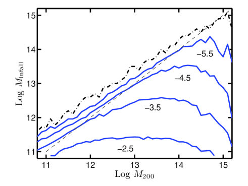
The usual way to implement ABM is to first populate subhaloes with galaxies, and only then to compute the auto correlation functions (CFs) of galaxies. In our approach there are many possible models, mainly depending on the different mass relations for satellite and central galaxies. Since computing the statistics of pairs is the most demanding computational step, it is not possible to scan a significant number of models in the usual technique. Here we present a new way of computing the CFs which is extremely efficient when many models are needed. We first compute the statistics of subhalo pairs, and save them as a function of and . Only then are the galaxy CFs computed. In this section we explain how the statistics of subhaloes is defined and computed, the next subsection discusses the way this information is used to model galaxies.
We want to constrain our models against the stellar mass function of galaxies. In order to do so we will use the mass function of central and satellite subhaloes:
| (4) |
| (5) |
Here is the volume of the simulation box, and are the numbers of central and satellite subhaloes respectively. In Fig. 1 we show the two dimensional mass function , for a model with . A similar behaviour as presented here is valid for , where the low-mass contour can vary by dex, and the contour of massive subhaloes is hardly affected.
In order to compute the CFs of galaxies, we start by computing the number of subhalo pairs, , for the total sample of subhaloes. In case both subhaloes within the pair are central subhaloes, we count this pair into :
| (6) |
Here , are the infall mass of the first and second subhaloes in the pair, and is the distance between these subhaloes within the - plane. Distances are computed only within the - plane in order to compute the projected auto-correlation function, as is described below. In practice we divide the range in Log and Log() into 100 and 50 bins respectively, and save as a multi-dimensional histogram.
In a similar way we define the pair statistics of central-satellite, and satellite-satellite subhaloes,
| (7) |
| (8) |
Note that for satellite subhaloes the number of pairs is saved as a function of both and . This is done in order to properly model the dependence of stellar mass on . It should be emphasized that the statistics of satellite subhaloes, i.e. , , , depend on the dynamical friction constant, , and on the location we adopt for unresolved subhaloes ( and from Eq. 3).
2.4 Definition of a model - domains in stellar mass
Previous studies have often used an analytic functional form to describe the relation between and . For example, Moster et al. (2010) suggested:
| (9) |
where are all constants. A straight forward way to extend this approach here would be to parameterize as a function of two variables, , and to use a different set of parameters for modeling central and satellite galaxies. However, this approach requires a priori knowledge of , and the resulting solutions might be restricted by the specific functional form chosen. This is especially true when is allowed to be different for satellite and central galaxies, so the freedom in its functional shape might be larger than what was found in previous studies (see the examples in section 3 below).
Here we suggest a new way to parameterize the relation between and , which is motivated by the observational data. The observed CFs of galaxies are computed over mass bins of width 0.5 dex in stellar mass (hereafter ‘domains’). For example, the CF for small mass galaxies is based on galaxies with stellar mass in the range
| (10) |
In order to model the CF in this range we only need to know the values of that correspond to . These are defined by:
| (11) |
Such constraints imply that in case of a smooth and monotonic , the ’boundaries’ of the domain correspond to curves within the plane. The relation that defines a boundary can thus be written as:
| (12) |
where is the curve function. All subhaloes that are located between & (their masses follow the constraint ) should contribute galaxies to the CF of the first domain.
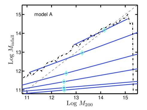
The standard abundance matching approach assumes that depends only on . In terms of our language, this means that the functions ’s are all constants, with no dependence on . In this work, we extend this assumption in two ways: we assume that might be a power-law for satellite galaxies444For central galaxies the values of are always very similar to so there is no added value in allowing the stellar mass of central galaxies to depend on ., and that for each domain there might be a different for central and satellite galaxies. This can be summarized as:
| Central subhaloes: | (13) | ||||
| Satellite subhaloes: |
Since the observed CFs are based on 5 domains in stellar mass, we need to specify ’s at 6 domain boundaries. Our model therefore includes 6 free parameters () for central subhaloes, and additional 12 parameters () for satellite galaxies. We choose to limit our models only to power-law dependence on following the results of paper I, and as a first order approximation. It will allow us to test how important the standard assumption of constant is. It might well be that a more complex behaviour would add a significant amount of freedom to the models.
In order to model the stellar mass function, we will use the same domains, and demand that the stellar mass function will be reproduced once integrated over each domain. This guarantees that in case it is needed, a detailed solution of the type exist. However, since our models allow the mass relation above to deviate between central and satellite galaxies, the detailed behaviour of within each domain is not well constrained. In general, there might be many different interpolations of the kind within each domain (between adjacent ’s). These will not change the computed CF, and will fit the observed stellar mass functions. The range in stellar mass for each domain is relatively small, so this freedom is negligible in comparison to the results we will show below.
In general, modeling a scatter in for a given and is possible within our formalism. However, it demands a detailed knowledge of the functional form, . This addition does not allow us to scan the different models in a very efficient way. We therefore do not treat such a scatter in this work. Nonetheless, the dependence of on for satellite galaxies results in a variation in as a function of . This effect will be discussed below.
2.5 How to compute CFs?
To summarize, each model in this work is defined by the following parameters:
- a)
-
The value of used in the dynamical friction formula, as defined by Eq. 2.
- b)
-
The values used in Eq. 3 for modeling the location of unresolved subhaloes. Alternatively, we use the location as given by the most bound particle.
- c)
-
For central subhaloes, 6 values of that define the domain boundaries (Eq.13).
- d)
-
For satellite subhaloes, 6 values of , and 6 values of that correspond to the boundaries.
Once the parameters , , are chosen, we construct the subhalo statistical functions and . The parameters in items (c) and (d) above are then used as integration limits for and . By integrating we compute the total number of subhaloes within the domain:
A similar integration of over each domain results in – the total number of pairs within each radial bin . The projected auto-correlation function, , is then defined as the deviation in the number of pairs from the average value per volume:
| (15) |
Here is the 2-dimensional area covered by the radial bin , and is the size of the simulation box in Mpc.
We have tested numerically that our methodology agrees with the standard ABM approach for various different models. In our approach the models are based on quantifying and only, so we do not construct a full realization of galaxies per each model. This is in contrast to standard ABM models, where a list of all subhaloes within a given simulation is necessary.
3 A few examples
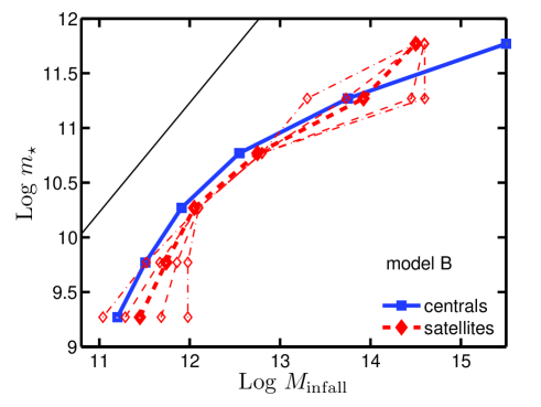
In this section we present a few specific models that were found using a large parameter search within our formalism. The details of the search will be presented in the next section. Here we discuss a few examples to demonstrate the parametrization needed for each model, and to highlight the variety of models that are able to fit both the stellar mass function and CFs.
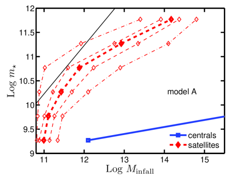
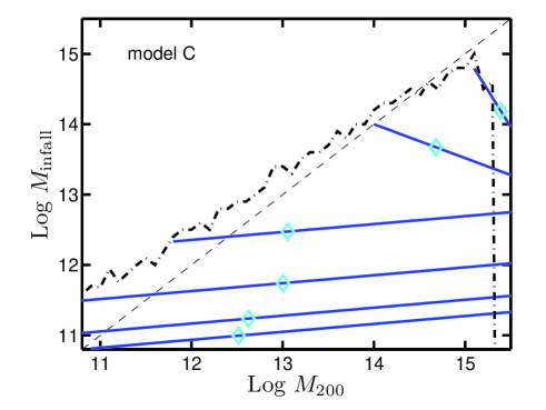
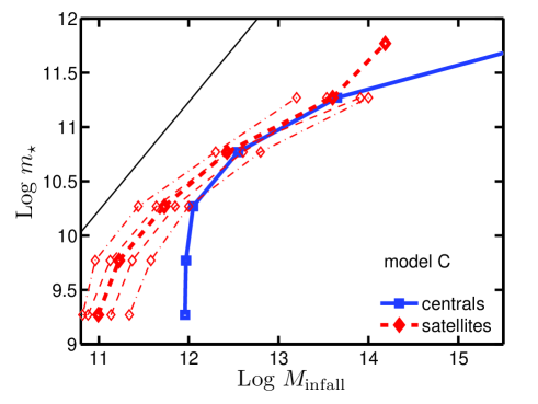
In Figs. 2 & 3 we present model , one example out of a family of models which are extreme with respect to the full population of models. In this model, is much higher for satellite subhaloes than for central subhaloes, for a given . The difference can reach a factor of 100 in stellar mass. As can be seen from Fig. 2, this model includes a relatively strong dependence of on , a feature that was originally seen in the SAMs analyzed in paper I, although less prominent. We note that previous ABM models were using only horizontal lines in the plane.
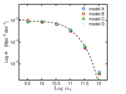
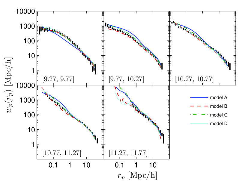
The CFs of model are plotted in Fig. 10, showing a reasonable match to the observed data, with an RMS deviation of 0.2 dex (more details on how we define this deviation can be found in section 4.1). Interestingly, the same model fits the stellar mass function well (see Fig. 7). These results suggest that even though model is extreme, it is broadly consistent with the observational constraints adopted here. However, Fig. 3 shows that this model violates the limit for satellite subhaloes. Assuming all baryons within each subhalo are converted into stars, the maximum stellar mass should equal . Model exceed this limit, and is therefore rejected and will not be considered as a valid model in what follows. It is plotted here to demonstrate that using our formalism, fitting both the stellar mass function and the CFs is not enough for constraining the maximum stellar mass per a given .
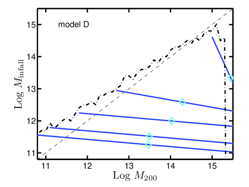
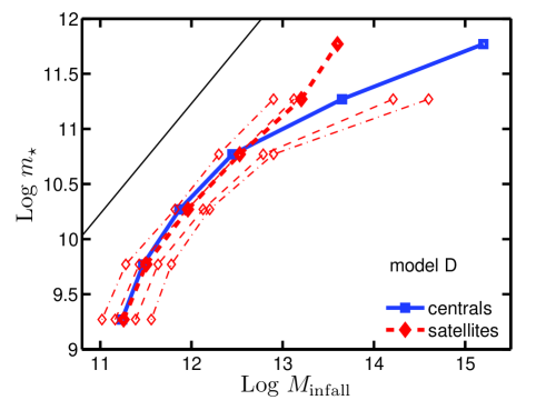
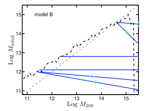
Models and are plotted in Figs. 4 & 5, and show a very different behaviour for low mass subhaloes. The difference for a given between these two models can reach a factor of 10 in for central and satellite subhaloes. Model shows a steep dependence of on for low mass central subhaloes. This means that for a given subhalo mass, the difference between for satellite and central galaxies might be very large, more than a factor of 10.
We emphasize that our definition of a ‘satellite’ versus ‘central’ is valid only for subhaloes. It might be that satellite subhaloes will host more massive galaxies than the central subhalo within the same group. In these cases the more massive galaxy in the group might be identified as a ‘central’ galaxy, although its host subhalo is defined as a ‘satellite’ here. In a recent study, Skibba et al. (2011), have estimated the fraction of haloes that host central galaxies that are not the most luminous in their group. Using a group catalog based on SDSS (Yang et al., 2007) they found that this fraction reaches 25 (40) per cent for low (high) mass haloes. Thus, a different identification of ‘central’ and ‘satellite’ may be used either in observational studies, or in the analysis of hydrodynamical simulations. In our models, the difference between satellite and central subhaloes is defined solely according to the dark-matter behaviour, and is motivated by the different merger history of subhaloes, and their final location.
From Fig. 5 it is evident that model predicts a non-negligible number of low mass subhaloes that host galaxies with very high stellar masses, including galaxies with . This shows again that our formalism cannot constrain the mass fraction that is locked in stars, in contrast to what has been claimed using more simplified ABM models (e.g. Behroozi et al., 2010; Guo et al., 2010).
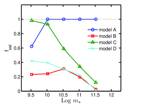
Model is a good example of a model with a very high abundance of satellite galaxies. Although the number of satellite subhaloes is smaller than central subhaloes at a given , different relations for central and satellite subhaloes might result in a high abundance of satellite galaxies. We plot the satellite fraction (the number of satellite galaxies out of all the galaxies of a given ) of all the models in Fig. 8. The satellite fraction changes significantly between the models. For model this fraction reaches unity at low stellar masses, while for models and it reaches a maximum value of and 0.4 respectively.
Model is shown in Fig. 6. It is an example for a model in which for satellites does not strongly depend on . In general, the slope of the relation, and the location where it turns over can be related to various processes in galaxy formation physics. Merger-rates, cooling, feedback and star-formation should all be combined in order to reproduce the observed relation (e.g. Shankar et al., 2006). Unless our more extreme models like model are ruled out by other observational constraints, our results indicate a large amount of freedom in modeling the above processes.
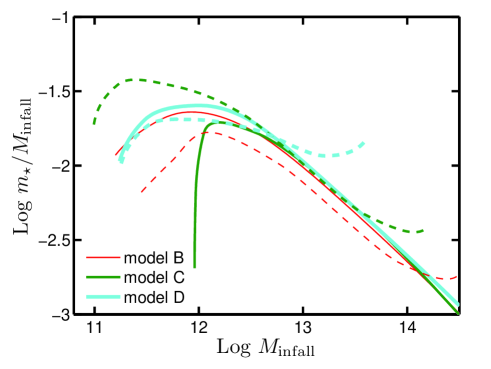
The stellar fractions, , for the few models presented here, are plotted in Fig. 9. The halo mass at which the global stellar fraction reaches a maximum can range from to . In model this efficiency is approximately constant for satellite galaxies as a function of , showing no global strong peak.
The CFs of all the models are shown in Fig. 10. Models fit the observed CFs to a good accuracy, below 0.1 dex RMS, while model is less accurate, reaching a level of 0.2 dex RMS. This demonstrates the importance of using this constraint here, in order to narrow down the range of accepted models. As can be seen from Fig. 7, all the models fit the stellar mass function well. Another point that should be emphasized regarding Fig. 10 is the small scale (Mpc) clustering of massive galaxies. The CF of different models shows variations at this regime, so it might be that extending the CF of the most massive domain into smaller radii will help to constrain the models. This will require a survey volume much larger than in the current SDSS survey.
4 Results
4.1 Search strategy
Each model within our formalism is defined by 21 free parameters, where 18 of them define the domains in stellar masses ( & from Eq. 13) used to compute the CF, 1 parameter fixes the time-scale for dynamical friction, and 2 parameters are responsible for the location of unresolved subhaloes. We were able to scan all possible options of the 18 parameters that govern the domains behaviour (within the resolution adopted here). In addition, we have tested five values in the range 0.1–10, and a few options for setting the location of unresolved subhaloes (see Appendix A and Table 1 for more details). In total, we have tested the stellar mass function for models, approximately out of them were tested against the observed CFs. More numerical details regarding the search algorithm can be found in Appendix B.
The values of and are saved numerically in fine bins. The choice of bin size is important for several reasons. First, the function depends on 5 different variables, so the number of bins we use for each variable is limited because of computer memory issues. Second, fine bins will require more evaluations of CFs, as the code checks automatically all possible options. This can slow our code dramatically. On the other hand, the bin size limits the search resolution: too big bins will not allow us to find all possible solutions. As a compromise between these requirements we have chosen the following bin sizes: is split into bins of 0.02 (0.1) dex for subhaloes with mass smaller (bigger) than , data per and are saved in bins of 0.1 dex. We use small bins for low mass because the typical difference between adjacent is smaller for small mass (see e.g., model above).
As described in section 2.4, the domain boundaries are defined using power-law relations. Writing Eq .13 in terms of Log mass gives . Our search algorithm checks all the possible values of according to the bins of . is modeled in terms of the line slope, . We sample in steps of degrees, over the range .
Each model is accepted if it follows the conditions below:
-
•
The model fits the stellar mass function of Li & White (2009) with an accuracy that is better than 20 per cent. This criterion is applied separately to each domain by integrating the stellar mass function over the domain range (0.5 dex in ). We have checked that the range of models shown below changes in a very minor way, when demanding a better fit that resembles the statistical errors from Li & White (2009) (these are 5,5,5,10,20 per cent for each domain, in order of increasing mass). Here we choose to use a constant accuracy of 20 per cent to account for systematic uncertainties in the stellar mass function (comparisons against other measurement can be found in Guo et al., 2010; Bernardi et al., 2010).
-
•
The model fits the logarithm of the observed CF (see Fig. 10) to better than an RMS value of 0.1 dex (26 per cent). This estimate is based on all points in the range Mpc , sampled in bins separated by 0.2 dex in Log(). In order to test the effect of this fit accuracy we also show results using 0.2 dex deviation. A detailed discussion of these issues is given below.
-
•
The model does not include individual points that deviate from the observed CF to more than a factor of 2.
-
•
The stellar mass function is fitted also for masses larger than the most massive domain (i.e. for ). This domain should include only 23 galaxies, when using the full Millennium simulation. Since this is a very small number, we allow our models to deviate an additional Poisson error from the nominal value. This means that the number of galaxies with masses larger than can have any value in the range [14, 34].
-
•
The stellar fraction (i.e. ) does not exceed the universal fraction of 0.17 for all subhaloes in the sample.
We adopt an accuracy of 0.1 and 0.2 dex for fitting the CFs due to the following reasons. First, the Millennium simulation being used here is based on a cosmological model with , higher than the most updated measurements of (Jarosik et al., 2011). This should give rise to some deviation between our models and observations. We find that there is a minimum deviation of 0.08 dex between all the models discussed here, and the observed CFs. Since this deviation is dominated by scales larger than 1 Mpc, it is probably related to the different cosmological model assumed. Second, due to the finite bins that are used for saving , the accuracy of our search algorithm is approximately 0.03 dex. As a result of the above, our minimum fit criterion is chosen to be 0.1 dex. However, since the error bars presented for the observed CFs are only statistical, it might be that systematic uncertainties would introduce errors that are larger than 0.1 dex. The CFs depend strongly on various galaxy properties like color, star-formation, and morphology (Li et al., 2006). Consequently, if the stellar masses of galaxies are systematically biased for galaxies of a given property (for example the high star-forming galaxies), this could change the CFs considerably. We therefore additionally consider a fitting criterion of 0.2 dex, to demonstrate the effect of the possible systematic uncertainties.
The minimum subhalo mass (), enforced by the Millennium simulation seems to limit our models (see models and above). It might be that using simulations of higher resolution will permit more models. The Millennium II simulation (Boylan-Kolchin et al., 2009) is a good candidate for such a study. However, high resolution simulations are naturally based on much smaller volume than what is being used here, resulting in a smaller statistical sample and non-negligible cosmic variance effects. Since our study is aiming at fitting the CFs to a high accuracy of 0.1 dex, we focus our study only on the Millennium simulation.
4.2 The mass relation
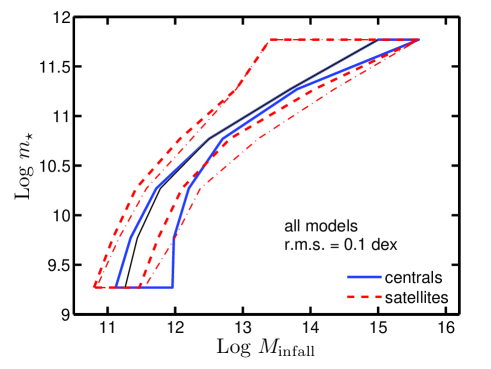
The main results of the parameter search are summarized in Figs. 11 and 12. In case we force the models to reproduce the observed CFs to a high accuracy of 0.1 dex, the range of accepted models occupies a region of 1 dex in the plane, as shown in Fig. 11. Interestingly, the uncertainty is small for central massive subhaloes. On the other hand, low mass central subhaloes can host galaxies with very low stellar masses. The range of accepted models increases significantly in Fig. 12, where the accuracy of fitting the CFs is set to 0.2 dex. We have checked that the distributions of models within the plotted envelope in Figs. 11-12 are roughly uniform, so the range of models is not affected by outliers.
The number of models presented in Fig. 11 and 12 is quite large. Each domain includes successful models in Fig. 11, and models in Fig. 12. We only take into account domains for which nearby from adjacent domains coincide, and the set of all 5 domains covers the full mass range. Due to the above, we compute the median for a given , which does not demand combinations of domains of different . Computing the opposite relation, median per a given , is much more complicated within our formalism. However, since the relation for central galaxies does not include any scatter, it represents a median per a given as well.
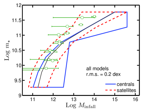
In our models, the stellar mass of satellite galaxies depends on their host halo mass, which correlates with the number of neighboring galaxies in observational studies. As a result, the range in the relation changes as a function of the host halo mass. This is shown in Fig. 11 by plotting the envelope of all median relation in the plane, but taking into account only galaxies that reside in clusters (their host halo mass is bigger than ). For these satellite galaxies, the range in for a given is larger than the one for all galaxies.
Fig. 12 includes the results of weak lensing analysis from Mandelbaum et al. (2006). These estimates are for the host halo mass555Mandelbaum et al. (2006) define the halo mass as the mass enclosed within a radius that corresponds to 180 times the mean density, this mass is higher than (see also Weinmann et al., 2006), but agrees quite well ( dex) with for central subhaloes used here. of central galaxies, and should be compared to the solid lines of our models. The square symbols represent a subsample of early type galaxies, while the circles correspond to late-type galaxies. As is mentioned in the figure caption, the fraction of late-type galaxies is very small at the most massive stellar mass bin (0.05).
Surprisingly, our results deviate from those of Mandelbaum et al. (2006) at the high mass end, even when the range of models is large, using an uncertainty of 0.2 dex in matching the CF. This is similar to what was found by previous ABM studies, summarized by Behroozi et al. (2010). Apparently, for a given value of , the weak lensing results constrain the host halo mass by providing mainly an upper threshold (the low values of the host halo often reach the universal baryonic fraction). The opposite seems to be true for central galaxies in our analysis. Deviations between the two studies can be due to various effects:
-
•
Mandelbaum et al. (2006) use a specific halo model for computing the lensing signal, which differs from the set of models being used here.
-
•
There is some uncertainty in their study owing to the width of the -distribution, for a given .
-
•
Their stellar mass estimates are based on Kauffmann et al. (2003) while the observations of Li & White (2009) use the method of Blanton & Roweis (2007). The difference between these estimates is discussed in both Li & White (2009) and Guo et al. (2010), and its effect on the stellar mass function is probably small. However, it might be that the difference between the methods are more significant for computing the CFs.
-
•
It might be that our range of models is too narrow, or that there are some systematic differences between the two approaches. This could be due to our search resolution, the assumed underlying cosmological models, or the assumed IMF.
A better, more self-consistent way to compare our results against weak lensing would demand a direct estimate of the lensing signal from our models. This can then be compared to the observed shear signal. Such an analysis is however outside the scope of this work. A recent study by Leauthaud et al. (2011) have used a model based on halo occupation distribution and demonstrated the strength of applying this additional constraint.
The results of Mandelbaum et al. (2006) indicate that the population of late-type massive central galaxies live inside haloes with lower masses than early-type galaxies. The difference between early and late type galaxies indicates that the scatter in the relation might be significant. A large scatter was also found by More et al. (2011), based on satellite kinematics. We do not model such a scatter for central galaxies in this study. Previous works (e.g. Moster et al., 2010) have shown that including a scatter modifies the relation at the massive end, such that for a given , decrease with increasing scatter. Interestingly, the results of Mandelbaum et al. (2006) reach the universal baryonic fraction, , for part of the galaxy population. This is very similar to what is found here, and can be seen in model (Fig. 5).
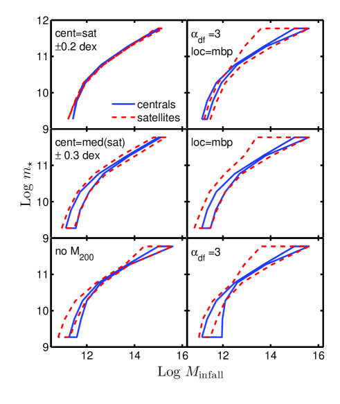
In Fig. 13 we plot various sub-samples of the models from Fig. 11, showing the influence of different parameters on the relation between and . Our results agree with previous studies in predicting a very tight relation, once satellite and central galaxies are considered to have very similar median relations (at the level of dex), and does not affect . This tight relation holds even though the models include the new ingredients related to and the location of satellite subhaloes. This proves that the dependence of on , and the difference between central and satellite galaxies, are responsible for the range of allowed models shown in Figs. 11-12.
It is worth noting that our models do not include solutions that have exactly the same mass relation for central and satellite galaxies, and can still fit the CFs to a level of 0.1 dex. The minimum deviation between central and satellite galaxies in the upper left panel of Fig. 13 is roughly 0.12 dex in . This small difference might be an artifact of the underlying cosmological parameters assumed by the Millennium simulation.
The models shown here use the two populations of galaxies to compensate for each other, keeping the overall relation relatively similar. This effect is shown in the middle left panel of Fig. 13. Once we force the models to have a similar median for satellite and central galaxies, the range of models decreases, especially at the high mass end. It might be that constraints on the differences between of the two populations, for a given , could be enforced ad-hoc. However, it is not clear what this limit should be. A reasonable demand would be that the full distribution of the two populations would overlap to some level, allowing a transition of central galaxies into satellites. This condition seems to be fulfilled by our models (see Figs. 4-6). Since we do not model a distribution for the of central galaxies, we do not explore this issue further here.
The effect of and satellite locations is explored in Fig. 13. It seems that both elements add freedom to our models, although the effect of satellite location is slightly stronger. Higher resolution cosmological simulations might help to constrain . However, these simulations are based on dark-matter only, while the results here are affected strongly by the baryonic components of galaxies (see e.g. Boylan-Kolchin et al., 2008; Jiang et al., 2008).
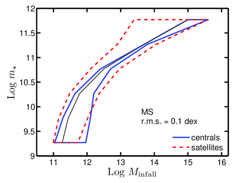
Lastly, in Fig. 14, we show the results of a parameter search when the reference CFs are not the observed ones, but instead are taken from one model out of the models tested here. The range of accepted models in this case is related to the internal degrees of freedom of the models, and is less related to the choice of the cosmological parameters, the method adopted for computing , or to the specific physical assumptions used in our formalism. The fact that Fig. 14 is similar to Fig. 11 indicates that the underlying cosmological model does not affect the range of acceptable models significantly. This is because here the reference CFs are based on the same cosmology, but use a specific model for the relation between and subhaloes. As was pointed out by Cacciato et al. (2009), the effect of the underlying cosmological model should be important when constraints from abundance and clustering of galaxies are combined with galaxy-galaxy lensing measurements. This issue should be further examined using an appropriate -body cosmological simulation.
5 Summary and discussion
In this work we have studied the relation between the stellar mass of galaxies () and the mass of their host subhaloes (). Our models are constrained by the abundance of galaxies, and their auto-correlation function (CF) at . We have shown that once the population of galaxies is broken into two sub-populations of central and satellite galaxies, the allowed range in the relation for each population reaches a factor of . The range of accepted models depends on the accuracy by which the models reproduce the observed abundance and clustering of galaxies. As was demonstrated in our previous work (Neistein et al., 2010, paper I), a different relation for central and satellite galaxies is expected in galaxy formation models, although the strength of the deviation cannot be constrained easily.
The shape of the relation has a large degree of freedom, resulting in a stellar fraction (the ratio between and ) that can peak anywhere between and . It can even be close to a constant as a function of for satellite galaxies. Interestingly, the stellar fraction can reach high values, comparable to the maximum universal value of 0.17, for low mass satellite galaxies residing in low mass haloes. Although it seems unlikely that the stellar fraction would exceed 0.17, our models are not able to constrain this ratio, and instead we are forced to use it as an ad-hoc constraint.
Our models are similar to the ‘abundance matching’ (ABM) approach, and are directly relating a galaxy with a specific to each subhalo within a large -body simulation. However, in comparison to previous studies, we include various additional ingredients for modeling satellite galaxies. Their stellar mass depends on both the host subhalo mass () and on the halo mass at , and might differ from the stellar mass of central galaxies of the same . We include subhaloes that have merged into more massive subhaloes at high-z but might host galaxies that will survive until , due to long dynamical friction time-scales. The location of these ‘unresolved’ subhaloes is set by either the location of their most bound particle, or by an analytical model. We found that the most important ingredient for fixing the range of accepted models is the way stellar masses for satellite galaxies are modeled.
A model with two populations of galaxies includes a large amount of freedom in matching the observed stellar mass function. We therefore constrain our models also against the observed auto-correlation function (CF) of galaxies. We developed a new formalism to compute the model CF based on the pair statistics of subhaloes. This enabled us to scan systematically a significant part of the parameter space. We have tested different ABM models, and estimated the CF for models that showed a good match to the stellar mass function. The accuracy by which we fit the CF affects significantly the range of accepted models within the plane. Consequently, a detailed study of the systematic uncertainties involved in this measurement is crucial in order to better constrain our models.
The range allowed in the relation might be larger than our prediction due to various effects. There are still a large number of models that we did not test here. These include complicated dependence of on the halo mass, different estimates for dynamical friction and satellite locations, higher resolution of the underlying -body simulation, different observed stellar mass functions (e.g. Bernardi et al., 2010), and modeling a random scatter in . On the other hand, the range of models might be modified once we use subhaloes from an -body simulation using the most up-to-date cosmological parameters. Previous estimates for the uncertainty in the relation were emphasizing the contribution from uncertainty in the stellar mass function, resulting in 0.25 dex (Behroozi et al., 2010). This uncertainty should be added to what we find here.
In this paper we have reproduced the abundance and clustering of galaxies only at when constraining the relation. It is not likely that data from higher redshifts would limit the relation to a narrow range. This is because the same uncertainties discussed here would be valid at high-z, in addition to the larger observational errors inherent at these redshifts. Moreover, once the relation is fixed at some redshift range, it is not straightforward to decide which models violate the physics of galaxy formation by linking galaxies at different epochs. For example, as we showed in paper I, the relation for satellite galaxies at the time of infall might already be different from the relation for central galaxies at the same epoch.
Our empirical results have implications for various aspects of galaxy formation. Guo et al. (2010) and Sawala et al. (2011) argued that stellar fractions at a fixed subhalo mass derived from basic ABM models are systematically lower than the results of detailed hydro-simulations. Our results that allow for a much larger spread of stellar mass at a fixed subhalo mass, are less definitive in this respect. This is especially true for dwarf galaxies, for which there is no available clustering data. An additional implication is related to the cumulative energy injected into the interstellar medium in a supernova feedback-constrained scenario. Shankar et al. (2006; see also Dekel & Woo, 2003) re-derived the expected trend of stellar and halo mass of the type . Here and is the fraction of surviving stellar mass. Based on the observed rather low stellar mass in haloes with inferred from a basic ABM model, they argued that supernova feedback appeared to be insufficient to remove the gas associated with the host halo. The results of this paper, however, show that some ABM models allow for much larger stellar mass fraction in low mass haloes, thus providing some hints towards the solution of this puzzling issue.
Another possible non-trivial consequence of our results concerns Halo Occupation Distribution (HOD) models. As outlined in e.g., Berlind & Weinberg (2002), this class of models is based on a parameterized conditional probability that a dark matter halo of virial mass contains galaxies. Adding prescriptions on the spatial distribution of subhaloes derived from accurate -body simulations, HOD models have been rather successful in reproducing the two-point correlation function of different classes of galaxies and at different redshifts. However, once we allow for a different ranking between satellite and central galaxies, as was found in this paper, the shape of might become rather different from its usual functional form. This could induce non-trivial degeneracies in these models, allowing for different occupation distributions that still match the data.
The methodology developed in this work can be used to study the clustering properties of AGNs, cold gas, and subsets of galaxies divided by e.g. luminosity or color. As was demonstrated here, our method already enabled us to better fit the observed stellar mass functions and CFs of all galaxies, with the current data sets. It might become more important when studying clustering properties of objects which tend to depend more strongly on environment, like the cold gas mass within galaxies. Our method may be able to shed some light on the limitations in modeling the observed high-z galaxies using standard halo models (Quadri et al., 2008; Tinker et al., 2010; Wake et al., 2011). In addition, it might be useful for future surveys with high quality data and a large survey volume, for which the simple abundance matching approach might not be flexible enough to provide an accurate fit to the data.
Improved constraints on the relation might be obtained from observational quantities, other than the stellar mass function and clustering used here. These might include: conditional stellar mass functions per halo mass (e.g. Yang et al., 2009a), satellite kinematics (More et al., 2011), weak lensing (Mandelbaum et al., 2006; Cacciato et al., 2009), star-formation histories, and dynamical tracers such as the velocity dispersion and circular velocity (e.g. Dutton et al., 2010). In addition, physically motivated models like hydrodynamical simulations or semi-analytic models are crucial to obtain insights on the difference between the evolution of satellite and central galaxies. More effort to understand the fundamental relation between the mass of subhaloes and galaxies is clearly needed both on the observational and theoretical side.
Acknowledgments
We thank the referee for a detailed and constructive report that helped to improve the presentation of this work. We also thank Peter Behroozi, Charlie Conroy, Umberto Maio, Rachel Mandelbaum, Risa Wechsler, and Simon White for useful discussions. The Millennium Simulation databases used in this paper and the web application providing online access to them were constructed as part of the activities of the German Astrophysical Virtual Observatory. FS acknowledges support from the Alexander von Humboldt Foundation. MBK acknowledges support from the Southern California Center for Galaxy Evolution, a multi-campus research program funded by the University of California office of research.
References
- Abazajian et al. (2009) Abazajian K. N., Adelman-McCarthy J. K., Agüeros M. A., Allam S. S., Allende Prieto C., An D., Anderson K. S. J., Anderson S. F., Annis J., Bahcall N. A., et al. 2009, ApJS, 182, 543
- Behroozi et al. (2010) Behroozi P. S., Conroy C., Wechsler R. H., 2010, ApJ, 717, 379
- Berlind & Weinberg (2002) Berlind A. A., Weinberg D. H., 2002, ApJ, 575, 587
- Bernardi et al. (2010) Bernardi M., Shankar F., Hyde J. B., Mei S., Marulli F., Sheth R. K., 2010, MNRAS, 404, 2087
- Binney & Tremaine (1987) Binney J., Tremaine S., 1987, Galactic dynamics
- Blanton & Roweis (2007) Blanton M. R., Roweis S., 2007, AJ, 133, 734
- Boylan-Kolchin et al. (2008) Boylan-Kolchin M., Ma C.-P., Quataert E., 2008, MNRAS, 383, 93
- Boylan-Kolchin et al. (2009) Boylan-Kolchin M., Springel V., White S. D. M., Jenkins A., Lemson G., 2009, MNRAS, 398, 1150
- Cacciato et al. (2009) Cacciato M., van den Bosch F. C., More S., Li R., Mo H. J., Yang X., 2009, MNRAS, 394, 929
- Colpi et al. (1999) Colpi M., Mayer L., Governato F., 1999, ApJ, 525, 720
- Conroy & Wechsler (2009) Conroy C., Wechsler R. H., 2009, ApJ, 696, 620
- Conroy et al. (2006) Conroy C., Wechsler R. H., Kravtsov A. V., 2006, ApJ, 647, 201
- Conroy et al. (2007) Conroy C., Wechsler R. H., Kravtsov A. V., 2007, ApJ, 668, 826
- Cooray & Sheth (2002) Cooray A., Sheth R., 2002, Phys. Rep., 372, 1
- Croton et al. (2006) Croton D. J., et al., 2006, MNRAS, 365, 11
- Davis et al. (1985) Davis M., Efstathiou G., Frenk C. S., White S. D. M., 1985, ApJ, 292, 371
- De Lucia & Blaizot (2007) De Lucia G., Blaizot J., 2007, MNRAS, 375, 2
- Dekel & Woo (2003) Dekel A., Woo J., 2003, MNRAS, 344, 1131
- Dutton et al. (2010) Dutton A. A., Conroy C., van den Bosch F. C., Prada F., More S., 2010, MNRAS, 407, 2
- Gao et al. (2005) Gao L., Springel V., White S. D. M., 2005, MNRAS, 363, L66
- Guo et al. (2010) Guo Q., White S., Li C., Boylan-Kolchin M., 2010, MNRAS, 404, 1111
- Harker et al. (2006) Harker G., Cole S., Helly J., Frenk C., Jenkins A., 2006, MNRAS, 367, 1039
- Hopkins et al. (2010) Hopkins P. F., Croton D., Bundy K., Khochfar S., van den Bosch F., Somerville R. S., Wetzel A., Keres D., Hernquist L., Stewart K., Younger J. D., Genel S., Ma C., 2010, ApJ, 724, 915
- Jarosik et al. (2011) Jarosik N., et al., 2011, ApJS, 192, 14
- Jiang et al. (2008) Jiang C. Y., Jing Y. P., Faltenbacher A., Lin W. P., Li C., 2008, ApJ, 675, 1095
- Kauffmann et al. (2003) Kauffmann G., et al., 2003, MNRAS, 341, 33
- Khochfar & Ostriker (2008) Khochfar S., Ostriker J. P., 2008, ApJ, 680, 54
- Khochfar & Silk (2009) Khochfar S., Silk J., 2009, ApJ, 700, L21
- Kravtsov et al. (2004) Kravtsov A. V., Berlind A. A., Wechsler R. H., Klypin A. A., Gottlöber S., Allgood B., Primack J. R., 2004, ApJ, 609, 35
- Leauthaud et al. (2011) Leauthaud A., et al., 2011, ArXiv e-prints, 1104.0928
- Li et al. (2006) Li C., Kauffmann G., Jing Y. P., White S. D. M., Börner G., Cheng F. Z., 2006, MNRAS, 368, 21
- Li & White (2009) Li C., White S. D. M., 2009, MNRAS, 398, 2177
- Mandelbaum et al. (2006) Mandelbaum R., Seljak U., Kauffmann G., Hirata C. M., Brinkmann J., 2006, MNRAS, 368, 715
- Mo et al. (2010) Mo H., van den Bosch F. C., White S., 2010, Galaxy Formation and Evolution
- Monaco et al. (2006) Monaco P., Murante G., Borgani S., Fontanot F., 2006, ApJ, 652, L89
- More et al. (2011) More S., van den Bosch F. C., Cacciato M., Skibba R., Mo H. J., Yang X., 2011, MNRAS, 410, 210
- Moster et al. (2010) Moster B. P., Somerville R. S., Maulbetsch C., van den Bosch F. C., Macciò A. V., Naab T., Oser L., 2010, ApJ, 710, 903
- Neistein & Weinmann (2010) Neistein E., Weinmann S. M., 2010, MNRAS, 405, 2717
- Neistein et al. (2010) Neistein E., Weinmann S. M., Li C., Boylan-Kolchin M., 2010, ArXiv e-prints: 1011.2492 (paper I)
- Pasquali et al. (2009) Pasquali A., van den Bosch F. C., Mo H. J., Yang X., Somerville R., 2009, MNRAS, 394, 38
- Purcell et al. (2007) Purcell C. W., Bullock J. S., Zentner A. R., 2007, ApJ, 666, 20
- Quadri et al. (2008) Quadri R. F., Williams R. J., Lee K., Franx M., van Dokkum P., Brammer G. B., 2008, ApJ, 685, L1
- Sawala et al. (2011) Sawala T., Guo Q., Scannapieco C., Jenkins A., White S., 2011, MNRAS, pp 64–+
- Shankar et al. (2006) Shankar F., Lapi A., Salucci P., De Zotti G., Danese L., 2006, ApJ, 643, 14
- Skibba & Sheth (2009) Skibba R. A., Sheth R. K., 2009, MNRAS, 392, 1080
- Skibba et al. (2011) Skibba R. A., van den Bosch F. C., Yang X., More S., Mo H., Fontanot F., 2011, MNRAS, 410, 417
- Springel et al. (2005) Springel V., White S. D. M., Jenkins A., Frenk C. S., Yoshida N., Gao L., Navarro J., Thacker R., Croton D., Helly J., Peacock J. A., Cole S., Thomas P., Couchman H., Evrard A., Colberg J., Pearce F., 2005, Nature, 435, 629
- Springel et al. (2001) Springel V., White S. D. M., Tormen G., Kauffmann G., 2001, MNRAS, 328, 726
- Tinker et al. (2010) Tinker J. L., Wechsler R. H., Zheng Z., 2010, ApJ, 709, 67
- Tinker et al. (2005) Tinker J. L., Weinberg D. H., Zheng Z., Zehavi I., 2005, ApJ, 631, 41
- Vale & Ostriker (2004) Vale A., Ostriker J. P., 2004, MNRAS, 353, 189
- van den Bosch et al. (2005) van den Bosch F. C., Tormen G., Giocoli C., 2005, MNRAS, 359, 1029
- von der Linden et al. (2007) von der Linden A., Best P. N., Kauffmann G., White S. D. M., 2007, MNRAS, 379, 867
- Wake et al. (2011) Wake D. A., et al., 2011, ApJ, 728, 46
- Wang et al. (2006) Wang L., Li C., Kauffmann G., De Lucia G., 2006, MNRAS, 371, 537
- Wang et al. (2007) Wang L., Li C., Kauffmann G., De Lucia G., 2007, MNRAS, 377, 1419
- Weinmann et al. (2010) Weinmann S. M., Kauffmann G., von der Linden A., De Lucia G., 2010, MNRAS, 406, 2249
- Weinmann et al. (2006) Weinmann S. M., van den Bosch F. C., Yang X., Mo H. J., 2006, MNRAS, 366, 2
- Weinmann et al. (2006) Weinmann S. M., van den Bosch F. C., Yang X., Mo H. J., Croton D. J., Moore B., 2006, MNRAS, 372, 1161
- Yang et al. (2009a) Yang X., Mo H. J., van den Bosch F. C., 2009a, ApJ, 695, 900
- Yang et al. (2009b) Yang X., Mo H. J., van den Bosch F. C., 2009b, ApJ, 693, 830
- Yang et al. (2007) Yang X., Mo H. J., van den Bosch F. C., Pasquali A., Li C., Barden M., 2007, ApJ, 671, 153
- York et al. (2000) York D. G., et al., 2000, AJ, 120, 1579
- Zehavi et al. (2005) Zehavi I., et al., 2005, ApJ, 630, 1
- Zentner et al. (2005) Zentner A. R., Berlind A. A., Bullock J. S., Kravtsov A. V., Wechsler R. H., 2005, ApJ, 624, 505
Appendix A The location of satellite galaxies
Here we describe the model we use for fixing the location of unresolved subhaloes. These subhaloes are not identified at , but can still host galaxies according to the dynamical friction estimate.
Consider a massive point particle subject to dynamical friction in an infinite mass distribution with density profile . In the limit of a circular orbit for the point particle and an isothermal profile () for the background density, the decay of the satellite’s orbit due to dynamical friction can be modeled analytically (eq. 7-25 of Binney & Tremaine 1987). Assuming that does not differ much from 2, we can follow the same arguments as Binney and Tremaine and find that the equation governing the decay rate for the specific angular momentum is
| (16) |
where is the Coulomb logarithm (assumed to be constant), is a constant, is the circular velocity, and is the frictional force. Using , and we get
| (17) |
Integrating, we obtain
| (18) |
where is the fraction of the initially estimated dynamical friction time-scale that has elapsed until , i.e. , and is the last redshift the subhalo was identified. For additional flexibility, we allow to vary as well, corresponding to the overall uncertainty in the dynamical friction time-scale:
| (19) |
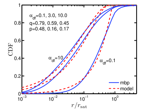
In Fig. 15 we compare the distribution of when using the most bound particle, against the model summarized in Eq. 19. Subhaloes from the simulation are chosen according to . For each unresolved subhalo we compute the location of the last identified most bound particle, this is shown in solid lines. Dashed lines show the results when using the model discussed above. For each value of plotted, we have optimized the parameters to get the best fit. Typically, is lower than 1 Mpc, and the CF measurements are reliable above kpc. Consequently, the difference between the plotted lines at is of less importance to this study. We have checked that the values of plotted here, agree with the location set by the most bound particle also when computing the CFs. Lastly, we list in Table 1 the combinations of satellite locations and that were used for the full parameter search discussed in section 4.
| Satellite location (p) | q | ||
|---|---|---|---|
| mbp | – | 0.1, 3, 8, 10 | |
| 0.1 | 0.4 | 0.1, 3 | |
| 0.14 | 0.6 | 0.1, 3, 10 | |
| 0.5 | 0.8 | 0.1, 1, 3, 10 | |
| 1.0 | 1.0 | 0.1, 1 | |
| 0.17 | 0.4 | 10 |
Appendix B Scanning the parameter space
As explained in section 4, each model within our formalism is defined using 18 free parameters that fix the five domains in stellar mass used here. There are additional three parameters that define the dynamical friction time scale (), and the location of unresolved subhaloes (). Even though this seems to be a huge parameter space, we managed to scan it systematically and with high resolution. In this section we explain the numerical details that allow this parameter search.
-
•
Searching the parameter space is done separately for the different domains of stellar mass. This reduces the number of independent parameters to those that define a domain (i.e. 6). Only in a later stage we search for solutions that combine a set of 5 domains that have mutual boundaries.
-
•
We search for solutions one domain after another, starting from the most massive one. At each domain we require that the model boundaries will coincide with an accepted model from the previous domain.
-
•
We first check that the stellar mass function meets the fitting criterion. Only after we have a solution for all the domains we check the fit to the CF.
-
•
Due to the number of bins we adopt for and each domain has optional combinations of . We first compute separately the contributions to the mass function (Eq. 2.5) from satellite and central subhaloes (). Only in a later stage we combine all the options to see which of them fits the data.
-
•
Before computing the CF we sort the different models such that there will be a minimum difference between neighboring models in the list. We then compute the CF using the ‘moving average’ scheme. This means that we do not compute the integral of Eq. 2.5 (and the related integral involving ) for each model, but only compute the incremental changes of this integral when going over the full list of models.
-
•
We compute CF values starting the smallest radius. After the CF is computed for each radius, we check whether the model fits the data. This allows us to quickly reject bad solutions.
Our algorithm is able to compute CF for each domain within a second, using one processor. In total, we have computed the CF for more than models. The CFs for all models are based on the full sample of subhaloes from the Millennium simulation.