Simulating the Effect of Non-Linear Mode-Coupling in Cosmological Parameter Estimation

Abstract

Fisher Information Matrix methods are commonly used in cosmology to estimate the accuracy that cosmological parameters can be measured with a given experiment, and to optimise the design of experiments. However, the standard approach usually assumes both data and parameter estimates are Gaussian-distributed. Further, for survey forecasts and optimisation it is usually assumed the power-spectra covariance matrix is diagonal in Fourier-space. But in the low-redshift Universe, non-linear mode-coupling will tend to correlate small-scale power, moving information from lower to higher-order moments of the field. This movement of information will change the predictions of cosmological parameter accuracy. In this paper we quantify this loss of information by comparing naïve Gaussian Fisher matrix forecasts with a Maximum Likelihood parameter estimation analysis of a suite of mock weak lensing catalogues derived from N-body simulations, based on the SUNGLASS pipeline, for a 2-D and tomographic shear analysis of a Euclid-like survey. In both cases we find that the 68% confidence area of the $\Omega_{m}-\sigma_{8}$ plane increases by a factor 5. However, the marginal errors increase by just 20 to 40%. We propose a new method to model the effects of nonlinear shear-power mode-coupling in the Fisher Matrix by approximating the shear-power distribution as a multivariate Gaussian with a covariance matrix derived from the mock weak lensing survey. We find that this approximation can reproduce the 68% confidence regions of the full Maximum Likelihood analysis in the $\Omega_{m}-\sigma_{8}$ plane to high accuracy for both 2-D and tomographic weak lensing surveys. Finally, we perform a multi-parameter analysis of $\Omega_{m},~{}\sigma_{8},~{}h,~{}n_{s},~{}w_{0}$ and $w_{a}$ to compare the Gaussian and non-linear mode-coupled Fisher matrix contours. The 6-D volume of the $1\sigma$ error contours for the non-linear Fisher analysis is a factor of 3 larger than for the Gaussian case, and the shape of the 68% confidence volume is modified. We propose that future Fisher Matrix estimates of cosmological parameter accuracies should include mode-coupling effects.

1 Introduction

Measuring cosmological parameters and the equation of state of dark energy to high accuracy is the goal of many current and upcoming experiments (e.g. PS1, DES, Euclid, HALO, LSST and WFIRST). Variables such as the size and depth of the survey (amongst other things) have a significant effect on the ability of a survey to constrain cosmological parameters. Consequently, significant effort must be spent in accurately predicting what these telescopes will see, well before construction begins. This will allow us to both to influence the design phase and to understand the capabilities of the instrument once the design has been set. In order to make predictions for these upcoming missions, statistical tools must be used to estimate the accuracy they will be able to achieve. The current standard for prediction uses the Fisher matrix methodology (Tegmark et al., 1997; Fisher, 1935). Traditionally, Fisher matrices have been generated with data covariance matrices that assume an underlying Gaussian matter and radiation distribution (Tegmark et al., 1997; Knox, 1997), which is accurate for CMB estimates when the Universe was still linear. However, this is not an accurate representation of the low-redshift Universe at smaller scales. Error bars generated using these Gaussian assumptions may be biased when compared with those generated using methods that account for the non-Gaussian, non-linear nature of the Universe.

In this paper we compare the $1\sigma$, two-parameter $\Omega_{m}-\sigma_{8}$ error estimates from the full maximum likelihood analyses with a Gaussian Fisher analysis. Using weak gravitational lensing power spectrum analysis of mock galaxy shear catalogues generated with the SUNGLASS pipeline (Kiessling et al., 2011), we show the importance of using accurate non-linear covariance matrices when estimating errors for future experiments. Analytic approximations of the correlation function covariance matrix under these assumptions have been shown to underestimate the errors on cosmic variance by a factor of up to $\sim 30$, which makes breaking the $\Omega_{m}-\sigma_{8}$ degeneracy more difficult (Semboloni et al., 2007). Simulations are able to provide accurate covariance matrices because they do not make assumptions about the underlying Gaussianity of the Universe and consequently, the resulting covariance matrices include the off-diagonal components.

Fisher matrix analyses are attractive because of their relative speed and minimal computational requirements when compared with maximum likelihood estimates. However, this is offset by the loss of information due to Gaussian assumptions in the generation of the Fisher matrix. To compensate for some of these Gaussian assumptions, we propose using a non-Gaussian weak lensing shear covariance matrix generated from simulations to generate the Fisher matrix. The resulting Fisher matrix still assumes a multivariate Gaussian parameter estimate distribution and power spectrum distribution. However, it now contains the non-linear information found in the off-diagonal components of the covariance matrix from the simulations, giving us a ‘non-linear’ Fisher matrix. In this paper, we will show the effect of this simple modification to the calculation of the Fisher matrix on the error estimates and compare this with the maximum likelihood and Gaussian Fisher error contours in the $\Omega_{m}-\sigma_{8}$ plane. We also perform a multi-parameter analysis of $\Omega_{m},~{}\sigma_{8},~{}h,~{}n_{s},~{}w_{0}$ and $w_{a}$ and compare the Gaussian and non-linear Fisher matrix error estimates.

It is possible to produce data vectors for covariance matrices by performing a simple 2-D binning of the galaxies in the survey. However, further information may be gained by splitting the distribution up in to redshift bins and performing a tomographic analysis (e.g. Hu, 1999, 2002; Jain & Taylor, 2003). In this work, we perform both 2-D and 3-bin tomographic analyses in order to generate covariance matrices that are used to calculate the maximum likelihood estimates and the Gaussian and non-linear Fisher matrices.

The outline of this paper is as follows. Section 2 will detail how the simulations and mock galaxy catalogues were generated. Section 3 will introduce the Fisher matrix formalism and the maximum likelihood formalism. Section 4 shows the results of the analyses on the maximum likelihood estimates and the Gaussian and non-linear Fisher matrices from the 2-D analyses in Section 4.1 and the tomographic analyses in Section 4.2. Section 4.4 compares the multi-parameter Gaussian and non-linear Fisher estimates. Finally, a summary of the findings will be presented in Section 5.

2 Details of the simulations

$N$	Area (sq deg)	$z_{\rm max}$	$n_{g}$/sq arcmin	$z_{\rm med}$
100	100	1.5	15	0.82

Table 1: Table of parameters for the mock galaxy shear catalogues used in this paper. $N$ is the number of independent lightcones, $z_{\rm max}$ is the maximum redshift in the lightcone and $n_{g}$/sq arcmin is the number of ‘galaxies’ per square arcmin in the catalogue and $z_{\rm med}$ is the median redshift of the catalogue. The suite of lightcones is used together to form a survey with an effective area of 10,000 sq. deg.

The suite of weak lensing simulations used in this work was generated using the SUNGLASS pipeline (for a detailed introduction, see Kiessling et al., 2011). We have 100 independent simulations generated with the cosmological N-body simulations code GADGET2 (Springel, 2005). The simulations were made with a flat concordance $\Lambda$CDM cosmology, consistent with the WMAP 7-year results (Jarosik et al., 2011): $\Omega_{m}=0.272$, $\Omega_{\Lambda}=0.728$, $\Omega_{b}=0.045$, $\sigma_{8}=0.809$, $n_{s}=0.963$ and $h=0.71$ in units of 100 km s^-1 Mpc^-1. There are $512^{3}$ particles in a box of $512h^{-1}$ Mpc which leads to a particle mass of $7.5\times 10^{10}{\rm M}_{\odot}$. The simulations were all started from a redshift of $z=60$ and allowed to evolve to the present with 26 snapshots being stored in redshifts $0.0\leq z\leq 1.5$.

Lightcones were generated through the simulation snapshots to determine the average convergence in an angular pixel using the ‘no radial binning’ method introduced in Kiessling et al. (2011):

$$\kappa_{p}(r_{s})=\sum_{k}\frac{K(r_{k},r_{s})}{\Delta\Omega_{p}\bar{n}(r_{k})r_{k}^{2}}-\int_{0}^{r_{s}}\!dr~{}K(r,r_{s}),$$ (1)

where $\bar{n}$ is the number density of particles in the simulation, $\Delta\Omega_{p}=\Delta\theta_{x}\Delta\theta_{y}$ is the pixel area, $r_{s}$ is the comoving radial distance of the lensing source plane and $r_{k}$ is the comoving radial distance of each particle, $k$, in the lightcone. $K(r,r_{s})$ is the scaled lensing kernel:

$$K(r,r_{s})=\frac{3H_{0}^{2}\Omega_{m}}{2c^{2}}\frac{(r_{s}-r)r}{r_{s}a(r)}.$$ (2)

The convergences were calculated using $2048^{2}$ azimuthal bins on source redshift planes that were separated by $z=0.1$ to create 15 planes from $0.0<z<1.5$. Once the convergences were calculated, shear values were determined in Fourier space, where the shear is given by $\gamma=\gamma_{1}+i\gamma_{2}$.

The shear and convergence values in these source redshift planes were interpolated back onto the individual particles in the lightcones to generate mock galaxy shear catalogues. The B-modes (the unphysical, imaginary component of the convergence) in the mock catalogues were calculated directly from the shear. These catalogues were then sampled to reproduce a standard galaxy redshift distribution (e.g. Efstathiou et al., 1991),

$$n(z)\propto z^{\alpha}\exp\left[-\left(\frac{z}{z_{0}}\right)^{\eta}\right],$$ (3)

where $z$ is the redshift, $z_{0}$, $\alpha$ and $\eta$ set the depth, low-redshift slope and high-redshift cut-off for a given galaxy survey. We take $\alpha=\eta=2$ and $z_{0}=0.78$ in this work, which gives a median redshift $z_{med}=0.82$. It is assumed that galaxies trace the dark matter distribution perfectly and the final mock galaxy shear catalogues contain 15 galaxies per square arcminute. There is no ellipticity noise in the catalogues, however there is a shot-noise contribution related to the discrete sampling of the particles in the mock catalogues. Table 1 summarises the mock galaxy catalogues used in this work.

3 Methodology

The shear, $\gamma$, convergence, $\kappa$, and B-mode, $\beta$, fields are related to each other in Fourier-space on a flat-sky by

$$\kappa(\mbox{\boldmath$\ell$})+i\beta(\mbox{\boldmath$\ell$})=e^{2i\varphi_{\ell}}[\gamma_{1}(\mbox{\boldmath$\ell$})+i\gamma_{2}(\mbox{\boldmath$\ell$})],$$ (4)

where $\varphi_{\ell}$ is the angle between the angular wave-vector and an axis on the sky. For each of the mock galaxy shear catalogues the shear, convergence, and B-mode auto- and cross-power spectra have been estimated. The tomographic weak lensing shear, convergence and B-mode power cross-spectra, for two different source redshifts $z$ and $z^{\prime}$, are given by

$$C_{\ell}^{\gamma\gamma}(z,z^{\prime}) = \langle\gamma_{1}(\boldsymbol{\ell},z)\gamma_{1}(\mbox{\boldmath$\ell$},z^{\prime})\rangle+\langle\gamma_{2}(\boldsymbol{\ell},z)\gamma_{2}(\mbox{\boldmath$\ell$},z^{\prime})\rangle,$$ (5)

$$C_{\ell}^{\kappa\kappa}(z,z^{\prime}) = \langle\kappa(\boldsymbol{\ell},z)\kappa(\mbox{\boldmath$\ell$},z^{\prime})\rangle,$$ (6)

$$C_{\ell}^{\beta\beta}(z,z^{\prime}) = \langle\beta(\boldsymbol{\ell},z)\beta(\mbox{\boldmath$\ell$},z^{\prime})\rangle.$$ (7)

The power spectra are related to each other by $C_{\ell}^{\gamma\gamma}(z,z^{\prime})=C_{\ell}^{\kappa\kappa}(z,z^{\prime})+C_{\ell}^{\beta\beta}(z,z^{\prime})$. The auto-spectra are calculated when $z^{\prime}=z$. In practice we bin the sources into redshift slices. For a survey that has $N_{z}$ slices the expectation-value of the tomographic shear power spectrum in redshift bins labeled $i$ and $j$, is given by

$$C^{\gamma\gamma}_{ij}(\ell)=\frac{9H_{0}^{4}\Omega_{m}^{2}}{4c^{4}}\int^{r_{\rm max}}_{0}\!\frac{dr}{a^{2}(r)}~{}P\left(\frac{\ell}{r},r\right)g_{i}(r)g_{j}(r),$$ (8)

(Kaiser, 1992; Joachimi & Schneider, 2009), where $r$ is the comoving distance, $r_{\rm max}$ is the maximum comoving distance and $P(\ell/r,r)$ is the 3D matter density power spectrum. The lensing efficiency function is

$$g_{i}(r)=\int_{r}^{r_{\rm max}}\!dr~{}p_{i}(r^{\prime})\left(1-\frac{r}{r^{\prime}}\right),$$ (9)

where $p_{i}$ is the normalised probability distribution of ‘galaxies’ in the bin.

When determining the angle averaged shear power spectrum in the simulations, we must take into consideration the conventions used in the Fourier transform software FFTW. Thus, the discretised tomographic shear power spectrum becomes

$$\frac{\ell(\ell+1)\widehat{C}_{ij}^{\gamma\gamma}(\ell)}{2\pi}=\!\!\!\sum_{\ell\,in\,shell}\!\!\!\!\frac{\gamma_{1}(\mbox{\boldmath$\ell$},z_{i})\gamma_{1}(\mbox{\boldmath$\ell$},z_{j})+\gamma_{2}(\mbox{\boldmath$\ell$},z_{i})\gamma_{2}(\mbox{\boldmath$\ell$},z_{j})}{n_{b}^{2}\Delta\ln\ell},$$ (10)

where $\widehat{C}_{\ell}^{\gamma\gamma}$ is the estimated power, $n_{b}$ is the total number of bins in the Fourier transform, $z_{i}$ is the $i^{th}$ redshift slice, and $\Delta\ln\ell$ is the thickness of a shell in log $\ell$-space. The modes in this power spectrum are corrected for mode discreteness errors by scaling by the expected number of modes. To compactify the notation we shall denote the tomographic shear power by $C^{\gamma\gamma}_{X}(\ell)$, where $X=(i,j)$ is a pair of redshift slices. For our 2-D analysis there is only one bin so $i=j$. Using the information from these power spectra, we have the the information required to make cosmological parameter estimates.

3.1 Shear power covariance matrix generation

The shear cross-spectra covariance matrix, $M^{XX^{\prime}}_{\ell\ell^{\prime}}$ is defined by

$$M^{XX^{\prime}}_{\ell\ell^{\prime}}=\langle\Delta C^{\gamma\gamma}_{X}(\ell)\Delta C^{\gamma\gamma}_{X^{\prime}}(\ell^{\prime})\rangle,$$ (11)

where $\Delta C^{\gamma\gamma}_{X}(\ell)=C^{\gamma\gamma}_{X}(\ell)-\langle C^{\gamma\gamma}_{X}(\ell)\rangle$ and angled-brackets denotes ensemble averaging. The covariance matrix is an important element of parameter estimation, containing information on the strength of the correlations between variates, in this case the shear power spectrum modes. The accuracy of this matrix improves by increasing the numbers of realisations included in the calculation of the matrix. For this work, 100 independent realisations of 2-D power spectra provides an accuracy of $\Delta C_{\ell}\sim 10\%$ (as shown in Figure 7 of Kiessling et al., 2011).

3.1.1 Gaussian covariance matrix

If the shear field is isotropic and we assume the shear field is Gaussian we can write down an equation for the tomographic shear power covariance matrix and make a correction for the fraction of the sky covered by the survey:

$$M^{ij,kl}_{\ell\ell^{\prime}}\!\!\!\!\! = \!\!\!\!\!\!\frac{\delta^{K}_{\ell\ell^{\prime}}}{(2\ell+1)f_{\mathrm{sky}}}\Big{(}[C_{ik}^{\gamma\gamma}(\ell)+N_{i}(\ell)\delta^{K}_{ik}][C_{jl}^{\gamma\gamma}(\ell)+N_{j}(\ell)\delta^{K}_{jl}]$$ (12)

$$\,\,\,+\,\,\,[C_{il}^{\gamma\gamma}(\ell)+N_{i}(\ell)\delta^{K}_{il}][C_{jk}^{\gamma\gamma}(\ell)+N_{j}(\ell)\delta^{K}_{jk}]\Big{)},$$

where $f_{\mathrm{sky}}$ is the fraction of the sky covered by the survey and $N_{\ell}$ is a shot-noise term due to intrinsic ellipticity in the shear field. For the purposes of this work although we have discrete galaxy density, we set the intrinsic shear variance to zero so that $N_{\ell}=0$. In principle our results can be combined with a Gaussian noise covariance to model different weak lensing surveys.

3.1.2 Simulation covariance matrix estimation

The covariance matrix of the tomographic shear power spectrum for the suite of mock galaxy shear catalogues is estimated by

$$M^{XX^{\prime}}_{\ell\ell^{\prime}}=\frac{1}{N-1}\sum_{N}\Delta C_{X}^{\gamma\gamma}(\ell)\Delta C_{X^{\prime}}^{\gamma\gamma}(\ell^{\prime}),$$ (13)

where $N$ is the number of mock catalogue realisations and here $\Delta C_{X}^{\gamma\gamma}(\ell)=\widehat{C}_{X}^{\gamma\gamma}(\ell)-\langle\widehat{C}_{X}^{\gamma\gamma}(\ell)\rangle$ where $\langle\widehat{C}_{X}^{\gamma\gamma}(\ell)\rangle$ is the ensemble average of the tomographic shear power spectrum across all realisations.

We calculate inverse covariance matrix using a singular value decomposition (SVD) on the covariance matrix (Press et al., 1992). However, the resulting inverse is biased due to noise. To correct for this, we multiply the inverse by a factor (Hartlap et al., 2007):

$$[\widehat{M}^{XX^{\prime}}_{\ell\ell^{\prime}}]^{-1}=\frac{N_{S}-N_{p}-2}{N_{S}-1}[M^{XX^{\prime}}_{\ell\ell^{\prime}}]^{-1},$$ (14)

where $N_{S}$ is the number of realisations, $N_{p}$ is the total number of bins in all of the power spectra and $[\widehat{M}^{XX^{\prime}}_{\ell\ell^{\prime}}]^{-1}$ is an unbiased estimation of the inverse covariance matrix.

3.2 Fisher matrix generation

The Fisher matrix is given by

$$F_{ij}=\frac{1}{2}\sum_{\ell\ell^{\prime}}\sum_{XX^{\prime}}\frac{\partial C^{\gamma\gamma}_{X}(\ell)}{\partial\theta_{i}}\left[\widehat{M}^{XX^{\prime}}_{\ell\ell^{\prime}}\right]^{-1}~{}\frac{\partial C^{\gamma\gamma}_{X^{\prime}}(\ell^{\prime})}{\partial\theta_{j}},$$ (15)

where $i$ and $j$ label cosmological parameters (e.g. $\Omega_{m}$ and $\sigma_{8}$) and the partial derivatives are the gradient of the expectation value of the shear power spectrum in parameter space. In order to determine that gradients of the power spectra, we use a five-point function (Abramowitz & Stegun, 1968, equation 25.3.6) and the ensemble average power spectra. The theoretical prediction for the power spectrum was generated using a code provided by Benjamin Joachimi (as tested in Kiessling et al., 2011; Joachimi & Schneider, 2009). This code uses the Smith et al. (2003) non-linear power spectrum estimate, the Eisenstein & Hu (1998) matter transfer function and a numerically calculated linear growth factor. All further theoretical power spectrum predictions in this paper were performed using this same code.

The Fisher matrix provides parameter estimates through two methods. The first by calculating the area of the Fisher matrix error ellipse that encloses a two-parameter 68% confidence limit in the two parameter plane. The inverse of this area is proportional to the Figure-of-Merit that is often quoted in studies (e.g. Albrecht et al., 2006; Wang, 2008; Albrecht et al., 2009; Slosar, 2010). The second is the single-parameter marginal errors, which are given by

$$\Delta\theta_{i}=\left[F^{-1}\right]_{ii}^{1/2}.$$ (16)

3.3 Maximum likelihood parameter estimation

To perform a maximum likelihood analysis on the suite of mock shear catalogues, we use a Gaussian likelihood estimator. Despite the fact that the simulations are non-Gaussian, using a Gaussian likelihood has been shown to produce accurate results (Kiessling et al., 2011). The likelihood is given by

$$L(\hat{C}_{\ell}^{\gamma\gamma}|\sigma_{8},\Omega_{m})=\frac{1}{(2\pi)^{N/2}({\rm det}\widehat{M}^{XX^{\prime}}_{\ell\ell^{\prime}})^{1/2}}\exp\left[-\frac{\chi^{2}}{2}\right],$$ (17)

where $N$ is the number of independent mock catalogue realisations, and

$$\chi^{2}=\sum_{\ell\ell^{\prime}}\sum_{XX^{\prime}}\Delta C_{X}^{\gamma\gamma}(\ell)\left[\widehat{M}^{XX^{\prime}}_{\ell\ell^{\prime}}\right]^{-1}\Delta C_{X^{\prime}}^{\gamma\gamma}(\ell^{\prime}),$$ (18)

where $\Delta C_{X}^{\gamma\gamma}(\ell)=\widehat{C}_{X}^{\gamma\gamma}(\ell)-\langle C_{X}^{\gamma\gamma}(\ell)\rangle$, and $\langle C^{\gamma\gamma}_{\ell}\rangle$ is the expected angular power spectrum given by equation (8). While this likelihood analysis is computationally expensive, it takes into account the full non-Gaussian and non-linear nature of the simulations and should provide the most accurate error estimates. The maximum likelihood is related to the Fisher matrix by

$$F_{ij}=\left\langle-\frac{\partial^{2}\ln L}{\partial\theta_{i}\partial\theta_{j}}\right\rangle.$$ (19)

4 Results

4.1 2-D two-parameter analysis

Figure 1: Mean 2-D shear power spectrum for the suite of unbinned mock galaxy shear catalogues.The smooth (red) line is the theoretical prediction for the power spectrum, the (black) line shows the mean power spectrum for the suite of mock catalogues with errors on the mean shown. The diagonal (dark blue) dashed line shows the shot noise prediction and the (magenta) triangles show the measured B-modes. The bottom panel shows the the percentage difference of the data from the expected power spectrum with errors.

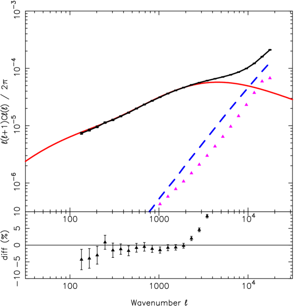
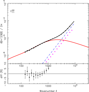
The first step to making parameter estimates from the mock galaxy shear catalogues is to determine the 2-D shear angular power spectra for each realisation. Figure 1 shows the mean power spectra from the suite with the (red) long line showing the theoretical prediction, the (black) line showing the mean measured power spectrum from the suite of catalogues with errors on the mean. The (magenta) triangles show the measured B-modes and the dashed (dark blue) line shows the shot-noise arising from discrete particle sampling in the mock catalogues. The bottom panel shows the percentage difference of the data from the expected power spectrum. The simulations recover the expected power spectrum within 5% between $150<\ell<2000$.

The shot noise prediction for these catalogues was determined by filling a suite of simulation volumes with randomly placed particles to mimic Poisson noise. The SUNGLASS pipeline was run on these noise simulations and the power spectrum of the mock catalogues is the dashed line in the figure. We know that the shot-noise in these catalogues is not purely Poissonian because the simulations start from a glass pre-initial distribution (White, 1994). However, the noise tends toward Poissonian as the simulations evolve. We are not able to model this noise accurately because it evolves with structures in the simulation (Baugh et al., 1995). Thus, this Poisson estimate should be a reasonable approximation for the noise in these catalogues.

A data-vector was constructed from the shear band-power spectra with wavenumbers from $150<\ell<1500$. From this, we estimated the covariance matrix in equation (13). Similarly, a Gaussian covariance matrix was generated using equation (12).

To test the effect of the non-Gaussian nature of the simulations covariance matrix, we looked at the diagonal components of both the simulation and Gaussian field covariance matrices and determined their $\Delta C_{\ell}$ values. For the case of the simulations this is simply the square root of the diagonal components. For the Gaussian field this is

$$\Delta C_{\ell}=\frac{\sqrt{2}C_{\ell}}{\sqrt{\ell(2\ell+1)f_{\rm sky}\Delta\ln\ell}}.$$ (20)

Figure 2: Diagonal components of the covariance matrix for the simulations (black line) and a Gaussian field with the same power spectrum (red dashed line).

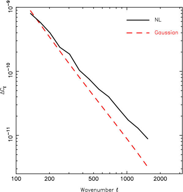
Figure 2 shows the diagonals of the covariance matrices as a function of wavenumber $\ell$. The (red) dashed line is from the Gaussian error and the (black) line is from the simulations. At low wavenumbers, which is still in the reasonably linear regime, the two errors agree reasonably well. However, in the higher wavenumber, non-linear regime, there is a factor of three difference between the errors, suggesting that the non-Gaussian contribution to the covariance is significant.

Fisher matrices in the $\Omega_{m}-\sigma_{8}$ plane were calculated using equation (15) for both the Gaussian and simulation covariance matrices. The Fisher matrices were multiplied by 100, the total number of independent mock catalogues, to provide an error estimate for a survey of 10,000 square degrees. Additionally, the maximum likelihood was calculated using the simulation covariance matrix and the likelihoods from the 100 mock catalogues were combined (as shown in Kiessling et al., 2011). For all of these calculations it is assumed that all other cosmological parameters are known.

In Figure 3 the two-parameter $1\sigma$ contours for the $\Omega_{m}-\sigma_{8}$ plane are shown. The inner (orange shaded) ellipse shows the Gaussian Fisher estimate, the outer (grey shaded) ellipse shows the non-linear Fisher estimate and the thick (black) line contour is the combined maximum likelihood estimate. The red point in the middle represents the fiducial $\Omega_{m}$ and $\sigma_{8}$ parameters. The size and shape of the simulation Fisher ellipse and the maximum likelihood contour are very similar, showing that the non-linear Fisher calculation is a good method for making future cosmological parameter estimates, provided the off-diagonal terms are included. The area of the non-linear Fisher estimate is 5.1 times larger than the area of the Gaussian Fisher estimate which is a clear indication that the off-diagonal terms in the covariance matrix are essential for accurate estimation of the parameter errors.

Figure 3: Comparison of the $1\sigma$ two-parameter contours for the $\Omega_{m}-\sigma_{8}$ parameters for Gaussian Fisher contour (inner orange shaded ellipse) with the non-linear Fisher contour (middle grey shaded ellipse) and the full maximum likelihood analysis (thick black line contour). The (red) point in the middle of the ellipses represents the fiducial $\Omega_{m}-\sigma_{8}$ parameters in this calculation.

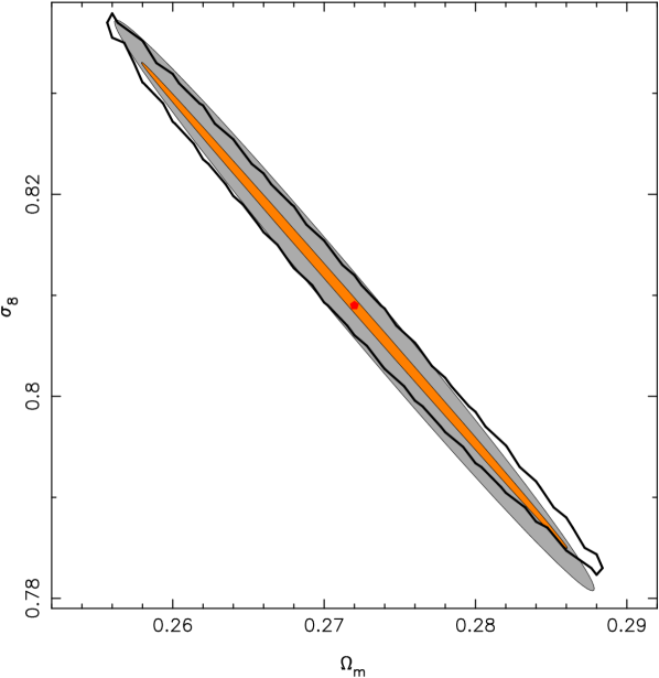
In addition to the area of the contours we also determined the marginal errors on the parameters from the Fisher matrices. The non-linear $\Omega_{m}$ marginal error is 1.23 times larger than the Gaussian marginal errors and $\sigma_{8}$ is 1.17 times larger. From Figure 2, we would expect the marginal errors to be much larger. However, the off-diagonal terms in the simulation covariance matrix act to reduce the marginal errors but increase the total area. This is demonstrated by setting the off-diagonal terms in the simulation covariance matrix are to zero. In this case the non-linear Fisher ellipse becomes far narrower but the marginal errors increase significantly.

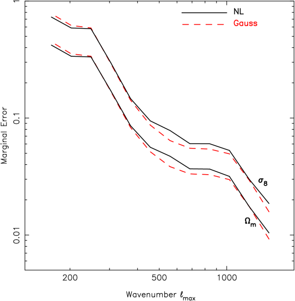
Figure 4 shows how the marginal errors change in the non-linear Fisher matrix as a function of maximum wavenumber $\ell_{\rm max}$. The marginal errors for both the non-linear and Gaussian Fisher matrices are remarkably similar across all values of $\ell_{\rm max}$ with the largest gain of information occurring for both $\Omega_{m}$ and $\sigma_{8}$ between $250<\ell_{\rm max}<500$ and again at $\ell_{\rm max}>1000$. This similarity is due to an effect that the off-diagonal components of the simulation covariance matrix are having on the error ellipse, as discussed earlier. This figure shows that if the marginal error is the value of interest, the Gaussian Fisher matrix appears to provide a result that is comparable with the error obtained with the non-linear Fisher error estimate at wavenumbers between $150<\ell_{\rm max}<1500$. However, when the errors are marginalised over two parameters, the area of the contours shows that the errors are being underestimated by a factor of five.

Figure 4: Marginal errors of $\Omega_{m}$ and $\sigma_{8}$ as a function of maximum wavenumber in the Fisher calculation. The dashed lines are the marginal errors on $\Omega_{m}$ as a function of maximum wavenumber $\ell_{\rm max}$ and the continuous lines are for $\sigma_{8}$.

4.2 Tomographic shear power

It is possible to perform the same analysis that was performed in Section 4.1 on tomographically-binned mock catalogues. Tomography introduces extra information into the analysis. In this analysis the suite of mock galaxy shear catalogues was split into three redshift bins; bin 1: $0.0\leq z\leq 0.5$, bin 2: $0.5<z\leq 1.0$ and bin 3: $1.0<z\leq 1.5$.

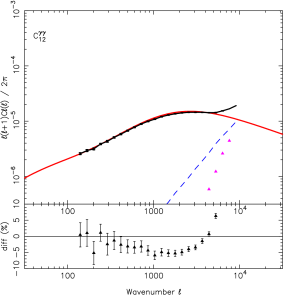
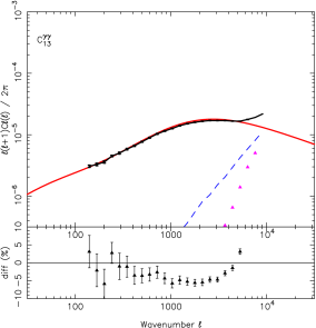
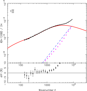
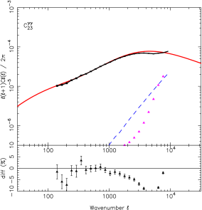
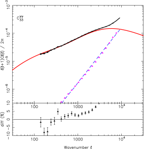
Figure 5 shows the auto- and cross-power spectra for the 3-bin tomographic analysis of the mock galaxy shear catalogues. If we first focus on the auto-power spectra ($C_{11},~{}C_{22}$ and $C_{33}$), we can see that the wavenumbers that we model accurately increase with redshift. For $C_{11}$, we find agreement for wavenumbers from $150<\ell<700$. The power spectra from $C_{22}$ and $C_{33}$ are slightly higher than the expected power spectrum but still within 3% and are reliable up to $\ell=1000$ before shot-noise becomes dominant.

The cross-bins $C_{12},~{}C_{13}$ and $C_{23}$ are damped which is due to the shot noise dominance in the lower redshift bin. Consequently, we only use the results of these power spectra up to the $\ell$ range accurately recovered by the auto-power spectra of the lower redshift bin.

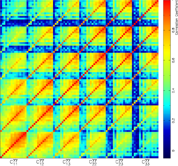
The power spectra in the auto- and cross-bins were turned into a data-vector with wavenumbers from $150<\ell<1800$ included. A data covariance matrix was generated and from this, the correlation coefficient matrix where the correlation coefficients are given by

$$r^{XX^{\prime}}_{\ell\ell^{\prime}}=\frac{\widehat{M}^{XX^{\prime}}_{\ell\ell^{\prime}}}{\sqrt{\widehat{M}^{XX}_{\ell\ell}\widehat{M}^{X^{\prime}X^{\prime}}_{\ell^{\prime}\ell^{\prime}}}}.$$ (21)

This matrix shows how (anti-)correlated each of the $\ell$ modes are.

Figure 6 shows the correlation coefficient matrix for the tomographic data vector. The ‘block’ nature to the matrix indicates each tomographic bin pair. Each of the blocks along the diagonal represents the auto-correlation between each of the tomographic power spectrum analyses. The off-diagonal blocks show the cross-correlations between the tomographic pair power spectra. As expected, the higher wavenumbers in each block are highly correlated. Additionally, the $C_{11}$ auto-power spectrum is highly correlated. The $C_{22}$ auto-power spectrum is significantly less correlated and the $C_{33}$ auto-power spectrum bin has very low correlations between the $\ell$ modes. The indication of this is that the lower redshift tomographic bins should contribute fewer power spectrum bins to a covariance matrix being used for any kind of analysis.

Figure 5: 2-D shear power spectra for a 3-bin tomography analysis of the mock galaxy shear catalogues. The long (red) line is the theoretical prediction for the shear power spectrum, the (black) line is the mean power spectrum for the 100 mock catalogues with errors on the mean, the (dark blue) dashed line is the shot noise estimate and the (magenta) triangles are the measured B-modes.

Figure 6: Correlation coefficient matrix for 3 tomographic bins. The matrix is arranged so that each sub-square is a tomographic bin pair.

With the information gained from these power spectra and the correlation coefficient matrix, we are able to assemble a data-vector that contains the $C_{\ell}$ from wavenumbers that are accurately reproducing the expected power spectrum and have a reasonably low correlation. Thus, we select 30 bins in total from the three auto-power spectra, with the highest wavenumber being around $\ell=1000$ and just 10 bins in total from the cross-power spectra, with the highest wavenumber being around $\ell=500$. A covariance matrix was generated using this data-vector. A full maximum likelihood analysis was performed with this covariance matrix and a non-linear Fisher matrix was also calculated. An equivalent Gaussian covariance matrix was also generated and the Gaussian Fisher matrix determined.

4.3 Two-parameter tomographic analysis

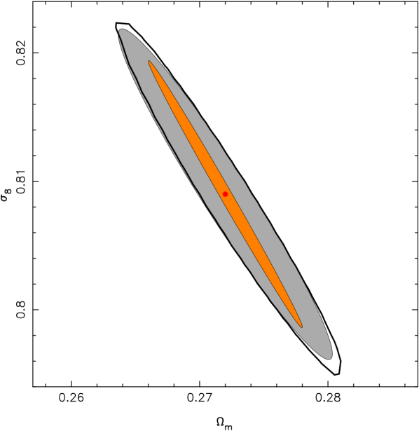
Figure 7 shows the $1\sigma$, two-parameter contours for the Gaussian Fisher (orange shaded ellipse) and the non-linear Fisher (grey shaded ellipse). The thick black line shows the simulation maximum likelihood analysis. As in the case for the 2-D analysis, the non-linear Fisher contour is very close to the maximum likelihood contour. The area of the non-linear Fisher contour is 5.1 times larger than the area of the Gaussian Fisher contour. The marginal error of the non-linear Fisher estimate is 1.39 times larger in $\Omega_{m}$ and 1.24 times larger in $\sigma_{8}$. These numbers are very similar to those calculated in the 2-D analysis.

The area of the contours and the size of the marginal errors in the tomographic Fisher and likelihood estimates is smaller than those in the unbinned analyses, showing that the tomographic analysis does indeed contain more information.

Figure 7: Comparison of the $1\sigma$, two-parameter contours for the $\Omega_{m}-\sigma_{8}$ parameters for the Gaussian Fisher contour (inner orange shaded ellipse), the simulation Fisher contour (middle grey shaded ellipse) and the full simulation maximum likelihood analysis (thick black line contour). The (red) point in the middle of the contours represents the fiducial $\Omega_{m}-\sigma_{8}$ parameters in this calculation.

4.4 Multi-parameter Fisher analysis

Tomographic Multi-Parameter Analysis
	NL	Gauss	Gauss / NL
$\Delta\Omega_{m}$	0.009	0.010	1.11
$\Delta\sigma_{8}$	0.019	0.021	1.11
$\Delta h$	0.198	0.352	1.78
$\Delta n_{s}$	0.143	0.201	1.41
$\Delta w_{0}$	0.107	0.129	1.21
$\Delta w_{a}$	0.343	0.584	1.70

Table 2: Marginal errors of a 3-bin tomographic, six-parameter Fisher matrix analysis using both Gaussian and non-linear Fisher matrices. For this configuration, the Gaussian marginal errors are always larger than the non-linear Fisher errors. However, the non-linear Fisher volume is 3.7 times larger than the Gaussian volume.

In the previous section, we showed that a Fisher matrix analysis in the $\Omega_{m}-\sigma_{8}$ plane accurately determines the errors on the parameters when a non-Gaussian data covariance matrix is used in the calculation. This was shown by comparing the 68% error contour with a maximum likelihood analysis of the simulation suite. In this Section we perform a Fisher matrix analysis over the cosmological parameters: $\Omega_{m},~{}\sigma_{8},~{}h,~{}n_{s},~{}w_{0}$ and $w_{a}$. Note that $\Omega_{\Lambda}=1-\Omega_{m}$. We compare the Gaussian Fisher analysis with the non-Gaussian (simulation) Fisher analysis. Based on the findings in the two-parameter analysis, we assume that the Fisher errors calculated with the simulation data covariance matrix are consistent with a maximum likelihood analysis of the simulations over the same multi-parameter space.

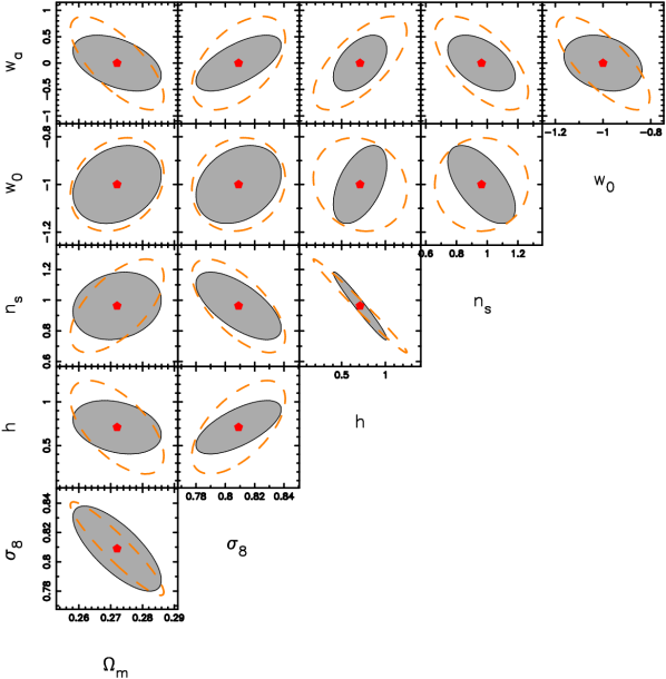
For a Euclid-like survey (Table 1), it makes little sense to perform a 2-D analysis over multiple parameters. We found that the size of the marginal errors was so large as to provide no constraining information (e.g. $\Delta w_{0}=11.3$ and $\Delta w_{a}=49.8$). However, the additional information provided by performing a tomographic analysis of the power spectra yielded far better constraints and illuminated some features of the Fisher matrix analysis that were not immediately obvious. Figure 8 shows the projected two-parameter, $1\sigma$ contours, marginalised over the the multiple parameters from the Fisher matrix analysis. The (red) point at the center shows the fiducial parameters used in the analysis, the (grey) shaded ellipses show the non-linear Fisher analysis and the dashed (orange) ellipses show the Gaussian Fisher analysis. In all cases, except the $\Omega_{m}-\sigma_{8}$ plane, the projected area of the Gaussian contours is larger than the area of the non-linear Fisher contours which gives the impression that the error estimates from the Gaussian Fisher analysis are more conservative the non-linear estimates. The marginal errors of the Gaussian contours are larger in all cases (Table 2). However, volume of the six-parameter space generated,

$$V\propto\sqrt{\det(F^{-1})},$$ (22)

shows that the non-linear Fisher volume is 3.7 times larger than the Gaussian volume, which is what we would expect given the off-diagonal terms included in the simulation data covariance matrix. The implication of this is that although the projected areas of the Gaussian Fisher appear larger, the overall volume is smaller. This can be explained with an example (in three dimensions for simplicity of explanation): Take a spherical ball and a thin plate with a slightly larger radius than the ball. If we look at the ball from any of the three axes, the area will appear to be the same circle in each projection. If we place the plate at a $45^{\circ}$ angle to each of the three axes and then look at it in projection, it will appear to have a larger area than the ball in all projections, however we know that the volume of the plate is far smaller than the ball. With this knowledge in hand, it is easy to see how misleading the projections of the Fisher matrices can be in these complex multiple-parameter spaces.

Figure 8: Multiple parameter Fisher analysis. The (grey) shaded ellipse is the non-linear Fisher contour and the (orange) dashed ellipse is the Fisher contour for the Gaussian Fisher matrix. The volume of the 6-dimensional space is larger in the simulation Fisher matrix, however some of the projected contours appear larger for the Gaussian Fisher matrix. This could be very misleading.

The eigenvalues and eigenvectors of the Fisher matrices were determined to find the equation for the plane with the most information in the full six-parameter space. For the Gaussian, this is:

$$X = 0.865~{}\Omega_{m}+0.498~{}\sigma_{8}+0.049~{}n_{s}+0.030~{}h-$$ (23)

$$0.035~{}w_{0}-0.006~{}w_{a},$$

and for the simulations:

$$Y = 0.841~{}\Omega_{m}+0.536~{}\sigma_{8}+0.034~{}n_{s}+0.028~{}h-$$ (24)

$$0.056~{}w_{0}-0.015~{}w_{a}.$$

When using the fiducial parameters,

$$X = 0.741,$$ (25)

$$Y = 0.771,$$ (26)

and the errors on the planes are $\Delta X=8.6\times 10^{-8}$ and $\Delta Y=1.4\times 10^{-6}$. This shows an order-of-magnitude difference in the thickness of the 6-D error ellipses.

5 Discussion and Conclusions

This paper makes a comparison between Fisher matrices in the $\Omega_{m}-\sigma_{8}$ plane and six-parameter Fisher matrices ($\Omega_{m},~{}\sigma_{8},~{}h,~{}n_{s},~{}w_{0}$ and $w_{a}$), generated using covariance matrices from a Gaussian random field and from full N-body simulations. The $1\sigma$ two-parameter contours from the two-parameter $\Omega_{m}-\sigma_{8}$ Fisher matrices are also compared with the contour from a maximum likelihood analysis of the full suite of simulations.

This work uses the SUNGLASS pipeline to generate 100 independent simulations of 512$h^{-1}$ Mpc with $512^{3}$ particles and a standard $\Lambda$CDM cosmology. The pipeline turns these simulations into 100 independent mock galaxy shear catalogues of 100 square degrees and a galaxy redshift distribution with a median of $z_{m}=0.82$ and 15 ‘galaxies’ per square arcminute. When these catalogues are combined, they provide an effective survey area of 10,000 sq. deg.

We perform both 2-D and 3-bin tomographic angular shear power spectrum analyses on each of the mock catalogues and generate covariance matrices from the resulting data-vectors. We also generate a Gaussian field covariance matrix to compare with the more realistic non-Gaussian analyses.

Using these covariance matrices, we generate Fisher matrices for the $\Omega_{m}-\sigma_{8}$ plane and show that the $1\sigma$, two-parameter contour for the non-linear Fisher matrix has an area that is 5.1 times larger than the theoretical prediction in both the 2-D and tomographic analyses. This indicates that the theoretical prediction is significantly under-predicting the errors on these parameters (the Figure-of-Merit is over-optimistic), even though their marginal errors are similar.

To quantify if the contours generated using the Fisher matrix are a reasonable estimate of the true errors, we compared these outputs with a combined maximum likelihood analysis of the full simulation suite. The resulting contours in both the 2-D and tomographic analyses closely matched the contours generated with the simulation Fisher matrix. From this, we can conclude that it is sensible to use a Fisher matrix analysis for parameter estimates, using a covariance matrix with all off-diagonal terms included.

Based on the success of the non-linear Fisher errors in matching the maximum likelihood estimates in the $\Omega_{m}-\sigma_{8}$ plane, we also perform both 2-D and 3-bin tomographic analyses to generate multi-parameter Fisher matrices of $\Omega_{m},~{}\sigma_{8},~{}h,~{}n_{s},~{}w_{0}$ and $w_{a}$. We compare the non-linear Fisher matrix with the Gaussian Fisher matrix under the assumption that the simulation Fisher matrices are providing accurate error estimates. With the survey parameters used in this paper, the 2-D analysis finds marginal errors on the parameters that are so large that they provide no constraining power.

The tomographic analyses find reasonable marginal errors and demonstrate the value of the additional information obtained from the tomography. However, the marginal errors of the Gaussian Fisher matrix are larger than the non-linear Fisher marginal errors for every parameter which is a counterintuitive result. We show that the projected contours from the Gaussian Fisher matrix are also larger than the non-linear Fisher matrix, even though the volume of the non-linear Fisher is 3.7 times larger than the Gaussian Fisher. This warns us that the projected Fisher contours can be misleading over complex multi-variate spaces and that larger 2-D contours do not necessarily indicate a larger error volume.

References

- Abramowitz & Stegun (1968) Abramowitz M., Stegun I. A., 1968, Handbook of mathematical functions with formulas, graphs and mathematical tables. New York: Dover, 1968, edited by Abramowitz, Milton; Stegun, Irene A.
- Albrecht et al. (2009) Albrecht A., Amendola L., Bernstein G., Clowe D., Eisenstein D., Guzzo L., Hirata C., Huterer D., Kirshner R., Kolb E., Nichol R., 2009, ArXiv e-prints
- Albrecht et al. (2006) Albrecht A., Bernstein G., Cahn R., Freedman W. L., Hewitt J., Hu W., Huth J., Kamionkowski M., Kolb E. W., Knox L., Mather J. C., Staggs S., Suntzeff N. B., 2006, ArXiv Astrophysics e-prints
- Baugh et al. (1995) Baugh C. M., Gaztanaga E., Efstathiou G., 1995, MNRAS, 274, 1049
- Efstathiou et al. (1991) Efstathiou G., Bernstein G., Tyson J. A., Katz N., Guhathakurta P., 1991, ApJ, 380, L47
- Eisenstein & Hu (1998) Eisenstein D. J., Hu W., 1998, ApJ, 496, 605
- Fisher (1935) Fisher R. A., 1935, J. Roy. Stat. Soc, 98, 39
- Hartlap et al. (2007) Hartlap J., Simon P., Schneider P., 2007, A&A, 464, 399
- Hu (1999) Hu W., 1999, ApJ, 522, L21
- Hu (2002) Hu W., 2002, Phys. Rev. D, 66, 083515
- Jain & Taylor (2003) Jain B., Taylor A., 2003, Physical Review Letters, 91, 141302
- Jarosik et al. (2011) Jarosik N., Bennett C. L., Dunkley J., et al. 2011, ApJS, 192, 14
- Joachimi & Schneider (2009) Joachimi B., Schneider P., 2009, A&A, 507, 105
- Kaiser (1992) Kaiser N., 1992, ApJ, 388, 272
- Kiessling et al. (2011) Kiessling A., Heavens A. F., Taylor A. N., Joachimi B., 2011, ArXiv e-prints
- Knox (1997) Knox L., 1997, ApJ, 480, 72
- Press et al. (1992) Press W. H., Teukolsky S. A., Vetterling W. T., Flannery B. P., 1992, Numerical recipes in FORTRAN. The art of scientific computing
- Semboloni et al. (2007) Semboloni E., van Waerbeke L., Heymans C., Hamana T., Colombi S., White M., Mellier Y., 2007, MNRAS, 375, L6
- Slosar (2010) Slosar A., 2010, ArXiv e-prints
- Smith et al. (2003) Smith R. E., Peacock J. A., Jenkins A., White S. D. M., Frenk C. S., Pearce F. R., Thomas P. A., Efstathiou G., Couchman H. M. P., 2003, MNRAS, 341, 1311
- Springel (2005) Springel V., 2005, MNRAS, 364, 1105
- Tegmark et al. (1997) Tegmark M., Taylor A. N., Heavens A. F., 1997, ApJ, 480, 22
- Wang (2008) Wang Y., 2008, Phys. Rev. D, 77, 123525
- White (1994) White S. D. M., 1994, arXiv:astro-ph/9410043