Abstract

I present the resummation of collinear and soft gluon corrections to single top quark production in the $t$ channel at next-to-next-to-leading logarithm (NNLL) accuracy using two-loop soft anomalous dimensions. The expansion of the resummed cross section yields approximate next-to-next-to-leading order (NNLO) cross sections. Numerical results for $t$-channel single top quark (or single antitop) production at the Tevatron and the LHC are presented, including the dependence of the cross sections on the top quark mass, and the uncertainties from scale variation and parton distributions. Combined results for all single top quark production channels are also given.

1 Introduction

The observation of single top quark production at the Tevatron [1, 2, 3, 4] and the re-discovery of top quarks at the LHC [5, 6] has increased the need for theoretical calculations of the cross sections for the relevant processes. The single top cross section is less than half of that for $t{\bar{t}}$ production while the backgrounds are considerable and make the extraction of the signal challenging. Single top quark production is important in probing electroweak theory and discovering new physics since the top quark mass is of the same order of magnitude as the electroweak symmetry breaking scale, and it provides opportunities for the study of the electroweak properties of the top quark.

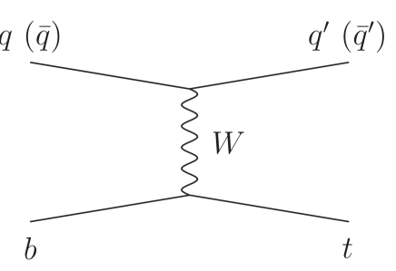
Single top quarks can be produced through three distinct partonic processes. One of them is the $t$-channel process that proceeds via the exchange of a space-like $W$ boson (Fig. 1), a second is the $s$-channel process that proceeds via the exchange of a time-like $W$ boson, and a third is associated $tW$ production (and the related $tH^{-}$ production). At both the LHC and the Tevatron the $t$-channel is numerically dominant. The $t$-channel partonic processes are of the form $qb\rightarrow q^{\prime}t$ and ${\bar{q}}b\rightarrow{\bar{q}}^{\prime}t$.

Figure 1: Leading-order $t$-channel diagram for single top quark production.

Calculations of next-to-leading order (NLO) corrections for $t$-channel production at the differential level have been known for some time [7] and recent updates and further studies of the NLO cross section have appeared in [8, 9, 10, 11]. Theoretical calculations for single top quark production beyond NLO that include higher-order corrections from next-to-leading-logarithm (NLL) soft-gluon resummation appeared in [12, 13, 14] for the three channels.

Recent advances in two-loop calculations with both massless [15] and massive [16] quarks now allow next-to-next-to-leading-logarithm (NNLL) resummation. More recently, calculations at NNLL accuracy have appeared for $s$-channel production [17] and $tW$ or $tH^{-}$ production [18]. Related NNLL calculations for $t{\bar{t}}$ production appeared in [19]. The present paper completes the NNLL results for top quark processes by studying $t$-channel single top quark production.

A different formalism for resummation based on soft-collinear effective theory (SCET) was used for $s$-channel production in Ref. [20] and for $t$-channel production in Ref. [21]. Different choices for the threshold kinematics variables were used in [20, 21] than in [17] and here. The authors of [20] have argued that their kinematics choice is more physical. However, they find that the soft-gluon contributions in the $s$ channel are small and their threshold expansion at NLO is not a good approximation to the exact NLO cross section at LHC energies. They also find smaller higher-order enhancements from soft gluons than in [17]. We disagree with their choices and conclusions (also, contrary to what is stated in [20], our expressions in [17] included the complete NNLL terms).

In our approach the soft-gluon contributions are dominant, in both $s$ and $t$ channels, and hence the resummation is more relevant and the NLO threshold expansion is a good approximation to the exact NLO result at both Tevatron and LHC energies. Hence, our complete NNLL higher-order corrections are also expected to be a better approximation. In this paper we use the same general formalism as presented in [13, 17]. Our new $t$-channel results at NNLL accuracy improve and update the earlier results in [13, 14].

In Section 2 we briefly describe the threshold resummation formalism and provide expressions for the two-loop soft anomalous dimension that leads to a NNLL resummed cross section. We expand the resummed cross section in powers of $\alpha_{s}$ and provide formulas for the soft-gluon corrections through next-to-next-to-leading order (NNLO). In Section 3 we present numerical results for single top quark (or single antitop) production via the $t$ channel at the Tevatron. Analogous results are provided for single top production at the LHC in Section 4 and for single antitop production at the LHC in Section 5. We conclude in Section 6 with a combination of the results in different channels for both Tevatron and LHC energies.

2 Two-loop resummation

In this section we present the resummed cross section for $t$-channel single top quark production. Details of the general resummation formalism for this process have been presented in [13].

For the partonic process $q(p_{1})+b(p_{2})\rightarrow q^{\prime}(p_{3})+t(p_{4})$, the kinematical invariants are $s=(p_{1}+p_{2})^{2}$, $t=(p_{1}-p_{3})^{2}$, $u=(p_{2}-p_{3})^{2}$, $s_{4}=s+t+u-m_{t}^{2}$, where $m_{t}$ is the top quark mass and we ignore the mass of the $b$-quark. Near the threshold of the partonic energy to produce the final state with the top quark, the quantity $s_{4}$, which measures distance from threshold, goes to zero. The threshold corrections then take the form of logarithmic plus distributions, $[\ln^{l}(s_{4}/m_{t}^{2})/s_{4}]_{+}$, where $l\leq 2n-1$ for the $n$-th order QCD corrections.

The resummation of the threshold logarithms is a consequence of the factorization of the cross section into hard, soft, and jet functions that describe, respectively, the hard scattering, noncollinear soft gluon emission, and collinear gluon emission from the partons in the process [22]. We take moments of the partonic cross section, ${\hat{\sigma}}(N)=\int(ds_{4}/s)\;e^{-Ns_{4}/s}{\hat{\sigma}}(s_{4})$. The moments of the logarithms of $s_{4}$ yield logarithms of the moment variable $N$, which exponentiate. The resummed partonic cross section in moment space is then

$${\hat{\sigma}}^{res}(N) = \exp\left[\sum_{i=1,2}E(N_{i})\right]\;\exp\left[{E^{\prime}}(N^{\prime})\right]\;\exp\left[\sum_{i=1,2}2\int_{\mu_{F}}^{\sqrt{s}}\frac{d\mu}{\mu}\;\gamma_{q/q}\left({\tilde{N}}_{i},\alpha_{s}(\mu)\right)\right]\;$$ (2.1)

$$\times\,{\rm Tr}\left\{H\left(\alpha_{s}(\sqrt{s})\right)\;\exp\left[\int_{\sqrt{s}}^{{\sqrt{s}}/{\tilde{N}^{\prime}}}\frac{d\mu}{\mu}\;\Gamma_{S}^{\dagger}\left(\alpha_{s}(\mu)\right)\right]\right.$$

$$\quad\left.\times\,S\left(\alpha_{s}(\sqrt{s}/{\tilde{N}^{\prime}})\right)\;\exp\left[\int_{\sqrt{s}}^{{\sqrt{s}}/{\tilde{N}^{\prime}}}\frac{d\mu}{\mu}\;\Gamma_{S}\left(\alpha_{s}(\mu)\right)\right]\right\}\,.$$

In Eq. (2.1) the first exponent resums collinear and soft gluon emission [23, 24] from the initial-state partons and it is given in the $\overline{\rm MS}$ scheme by

$$E(N_{i})=\int^{1}_{0}dz\frac{z^{N_{i}-1}-1}{1-z}\;\left\{\int_{1}^{(1-z)^{2}}\frac{d\lambda}{\lambda}A\left(\alpha_{s}(\lambda s)\right)+D\left[\alpha_{s}((1-z)^{2}s)\right]\right\}\,.$$ (2.2)

Here $N_{1}=N[(m_{t}^{2}-u)/m_{t}^{2}]$ and $N_{2}=N[(m_{t}^{2}-t)/m_{t}^{2}]$. The quantity $A$ has a perturbative expansion, $A=\sum_{n}(\alpha_{s}/\pi)^{n}A^{(n)}$. Here $A^{(1)}=C_{F}$ with $C_{F}=(N_{c}^{2}-1)/(2N_{c})$ where $N_{c}=3$ is the number of colors, while $A^{(2)}=C_{F}K/2$ with $K=C_{A}\;(67/18-\pi^{2}/6)-5n_{f}/9$ [25], where $C_{A}=N_{c}$, and $n_{f}=5$ is the number of light quark flavors.

Also $D=\sum_{n}(\alpha_{s}/\pi)^{n}D^{(n)}$, where in Feynman gauge $D^{(1)}=0$ and [26]

$$D^{(2)}=C_{F}C_{A}\left(-\frac{101}{54}+\frac{11}{6}\zeta_{2}+\frac{7}{4}\zeta_{3}\right)+C_{F}n_{f}\left(\frac{7}{27}-\frac{\zeta_{2}}{3}\right)$$ (2.3)

where $\zeta_{2}=\pi^{2}/6$ and $\zeta_{3}=1.2020569\cdots$.

The second exponent in Eq. (2.1) resums soft and collinear corrections [23, 24, 27, 28] from the final-state massless quark and it is given by

$${E^{\prime}}(N^{\prime})=\int^{1}_{0}dz\frac{z^{N^{\prime}-1}-1}{1-z}\;\left\{\int^{1-z}_{(1-z)^{2}}\frac{d\lambda}{\lambda}A\left(\alpha_{s}\left(\lambda s\right)\right)+B\left[\alpha_{s}((1-z)s)\right]+D\left[\alpha_{s}((1-z)^{2}s)\right]\right\}\,,$$ (2.4)

where $N^{\prime}=N(s/m_{t}^{2})$ and $A$ and $D$ are defined above. Here $B=\sum_{n}(\alpha_{s}/\pi)^{n}B^{(n)}$ with $B^{(1)}=-3C_{F}/4$ and

$$B^{(2)}=C_{F}^{2}\left(-\frac{3}{32}+\frac{3}{4}\zeta_{2}-\frac{3}{2}\zeta_{3}\right)+C_{F}C_{A}\left(-\frac{1539}{864}-\frac{11}{12}\zeta_{2}+\frac{3}{4}\zeta_{3}\right)+n_{f}C_{F}\left(\frac{135}{432}+\frac{\zeta_{2}}{6}\right).$$ (2.5)

In the third exponent the parton-density anomalous dimension $\gamma_{q/q}$ controls the factorization scale, $\mu_{F}$, dependence of the cross section. We write $\gamma_{q/q}=-A\ln{\tilde{N}}_{i}+\gamma_{q}$ where $A$ was defined above, ${\tilde{N}}_{i}=N_{i}e^{\gamma_{E}}$ with $\gamma_{E}$ the Euler constant, and $\gamma_{q}=\sum_{n}(\alpha_{s}/\pi)^{n}\gamma_{q}^{(n)}$ where $\gamma_{q}^{(1)}=3C_{F}/4$.

$H$ is the hard-scattering function while $S$ is the soft function describing noncollinear soft gluon emission [22]. The evolution of the soft function is controlled by the soft anomalous dimension $\Gamma_{S}$. The functions $H$, $S$, and $\Gamma_{S}$ are matrices in a basis consisting of color exchange, and we take the trace of the product involving these matrices in Eq. (2.1). For the $t$-channel process with color indices $a+b\rightarrow c+d$ we choose the color basis $e_{1}=\delta_{ac}\delta_{bd}$ and $e_{2}=T^{e}_{ca}T^{e}_{db}$. We write the perturbative series for the soft anomalous dimension as $\Gamma_{S}=\sum_{n}(\alpha_{s}/\pi)^{n}\Gamma_{S}^{(n)}$. Because of the simple color structure of the hard scattering for single top $t$-channel production, the hard and soft matrices take a very simple form and only the first diagonal element of the one-loop soft anomalous dimension matrix, $\Gamma_{S\,11}^{(1)}$, is needed in the NNLO expansion at NLL accuracy.

By expanding the resummed cross section, Eq. (2.1), in powers of $\alpha_{s}$ we derive fixed-order corrections, thus avoiding the prescription ambiguity that a fully resummed cross section entails to avoid the infrared singularity. This has been our approach in Refs. [12, 13, 14, 17, 18, 19].

The NLO soft-gluon corrections to the differential cross section are

$$\frac{d^{2}{\hat{\sigma}}^{(1)}}{dt\,du}=F^{B}\frac{\alpha_{s}(\mu_{R})}{\pi}\left\{c_{3}\left[\frac{\ln(s_{4}/m_{t}^{2})}{s_{4}}\right]_{+}+c_{2}\left[\frac{1}{s_{4}}\right]_{+}\right\}\,,$$ (2.6)

where $F_{B}$ is the Born term [13] and $\mu_{R}$ is the renormalization scale. The leading coefficient is $c_{3}=3C_{F}$. The next-to-leading coefficient, $c_{2}$, can be written as $c_{2}=T_{2}+c_{2}^{\mu}$, where $T_{2}$ represents the scale-independent part of $c_{2}$ and $c_{2}^{\mu}$ has all the scale dependence. Here

$$T_{2}=2{\Gamma}_{S\,11}^{(1)}-\frac{3}{4}C_{F}-2C_{F}\ln\left(\frac{(t-m^{2}_{t})(u-m^{2}_{t})}{m_{t}^{4}}\right)-3C_{F}\ln\left(\frac{m_{t}^{2}}{s}\right)$$ (2.7)

and

$$c_{2}^{\mu}=-2C_{F}\ln\left(\frac{\mu_{F}^{2}}{m_{t}^{2}}\right)\,.$$ (2.8)

The required element $\Gamma_{S\,11}^{(1)}$ of the one-loop soft anomalous dimension matrix for $t$-channel single-top production, necessary for NLL accuracy, was calculated first in Ref. [13] in axial gauge. The calculation involves one-loop eikonal diagrams with vertex corrections and a self-energy correction for the top quark line. The soft anomalous dimension is determined from the coefficients of the ultraviolet poles in dimensional regularization. In this paper we use the Feynman gauge and thus the result takes the slightly different form

$${\Gamma}_{S\,11}^{(1)}=C_{F}\left[\ln\left(\frac{-t}{s}\right)+\ln\left(\frac{m_{t}^{2}-t}{m_{t}\sqrt{s}}\right)-\frac{1}{2}\right]\,.$$ (2.9)

This change is of course compensated by different expressions for the $D$ term in Eqs. (2.2) and (2.4) than those used in [13] so that the final result for the resummed cross section is identical in the two gauges, as expected.

If we denote by $c_{1}$ the coefficient of the $\delta(s_{4})$ corrections in the NLO cross section, then we can calculate the scale-dependent part, $c_{1}^{\mu}$, from our resummation formalism

$$c_{1}^{\mu}=\left[C_{F}\ln\left(\frac{(t-m^{2}_{t})(u-m^{2}_{t})}{m_{t}^{4}}\right)-\frac{3}{2}C_{F}\right]\ln\left(\frac{\mu_{F}^{2}}{m_{t}^{2}}\right)\,.$$ (2.10)

The rest of the $c_{1}$ terms are found in the complete NLO calculation [7].

The off-diagonal one-loop elements of the soft anomalous dimension matrix are needed in the NNLO expansion at NNLL accuracy. We find

$$\Gamma_{S\,21}^{(1)}=\ln\left(\frac{u(u-m_{t}^{2})}{s(s-m_{t}^{2})}\right)\;,\quad\quad\Gamma_{S\,12}^{(1)}=\frac{C_{F}}{2N_{c}}\,\Gamma_{S\,21}^{(1)}\,.$$ (2.11)

The two-loop soft anomalous dimension is calculated by analyzing all the relevant two-loop diagrams (c.f. [16, 17, 18]). For the NNLO expansion at NNLL accuracy we need to determine the matrix element $\Gamma_{S\,11}^{(2)}$. We find

$$\Gamma_{S\,11}^{(2)}=\frac{K}{2}\Gamma_{S\,11}^{(1)}+C_{F}C_{A}\frac{(1-\zeta_{3})}{4}$$ (2.12)

where $K$ is the two-loop constant defined previously. The two-loop result in Eq. (2.12) is written in terms of the one-loop matrix element $\Gamma_{S\,11}^{(1)}$, Eq. (2.9).

With these two loop results, we next calculate the NNLO soft-gluon corrections. The corrections, written in terms of the various coefficients and soft anomalous dimensions defined above, take the form

$$\frac{d^{2}{\hat{\sigma}}^{(2)}}{dt\,du}=F^{B}\frac{\alpha_{s}^{2}(\mu_{R}^{2})}{\pi^{2}}\left\{\frac{1}{2}c_{3}^{2}\left[\frac{\ln^{3}(s_{4}/m_{t}^{2})}{s_{4}}\right]_{+}+\left[\frac{3}{2}c_{3}\,c_{2}-\frac{\beta_{0}}{4}c_{3}+C_{F}\frac{\beta_{0}}{8}\right]\left[\frac{\ln^{2}(s_{4}/m_{t}^{2})}{s_{4}}\right]_{+}\right.$$

$${}+\left[c_{3}\,c_{1}+c_{2}^{2}-\zeta_{2}\,c_{3}^{2}-\frac{\beta_{0}}{2}T_{2}+\frac{\beta_{0}}{4}c_{3}\ln\left(\frac{\mu_{R}^{2}}{m_{t}^{2}}\right)+\frac{3}{2}C_{F}\,K-\frac{3}{16}C_{F}\,\beta_{0}+4\Gamma_{S\,12}^{(1)}\,\Gamma_{S\,21}^{(1)}\right]\left[\frac{\ln(s_{4}/m_{t}^{2})}{s_{4}}\right]_{+}$$

$${}+\left[c_{2}\,c_{1}-\zeta_{2}\,c_{3}\,c_{2}+\zeta_{3}\,c_{3}^{2}+\frac{\beta_{0}}{4}c_{2}\,\ln\left(\frac{\mu_{R}^{2}}{s}\right)-\frac{\beta_{0}}{2}C_{F}\ln^{2}\left(\frac{m_{t}^{2}-t}{m_{t}^{2}}\right)-\frac{\beta_{0}}{2}C_{F}\ln^{2}\left(\frac{m_{t}^{2}-u}{m_{t}^{2}}\right)\right.$$

$$\quad{}-C_{F}\,K\,\ln\left(\frac{(m_{t}^{2}-u)(m_{t}^{2}-t)}{m_{t}^{4}}\right)+B^{(2)}+3D^{(2)}+C_{F}\frac{\beta_{0}}{4}\ln^{2}\left(\frac{\mu_{F}^{2}}{s}\right)-C_{F}\,K\ln\left(\frac{\mu_{F}^{2}}{s}\right)$$

$$\quad{}+\frac{3\beta_{0}}{8}C_{F}\ln^{2}\left(\frac{m_{t}^{2}}{s}\right)-C_{F}\left(\frac{K}{2}-\frac{3}{16}\beta_{0}\right)\ln\left(\frac{m_{t}^{2}}{s}\right)+2\Gamma_{S\,11}^{(2)}$$

$$\quad\left.\left.{}+\left(4\,\Gamma_{S\,12}^{(1)}\,\Gamma_{S\,21}^{(1)}+4\,(\Gamma_{S\,11}^{(1)})^{2}\right)\ln\left(\frac{m_{t}^{2}}{s}\right)\right]\left[\frac{1}{s_{4}}\right]_{+}\right\}\,$$ (2.13)

where $\beta_{0}=(11C_{A}-2n_{f})/3$ is the lowest-order beta function.

This expression, Eq. (2.13), extends the results in Ref. [13] from NLL to NNLL accuracy for $t$-channel single top production and it is the analog of the $s$-channel NNLL results in Ref. [17] and the $tW$ and $tH^{-}$ NNLL results in Ref. [18].

3 Single top or single antitop $t$-channel production at the Tevatron

We now use the previous theoretical expressions to study $t$-channel single top production at the Tevatron, noting that the results for single antitop production at the Tevatron are identical. We add the NNLO corrections in Eq. (2.13) to the NLO cross section and thus derive approximate NNLO cross sections at NNLL accuracy. We use the MSTW2008 NNLO [29] parton distribution functions (pdf), as we also did in [17, 18].

Figure 2: The approximate NNLO cross section for single top quark production at the Tevatron with $\sqrt{S}=1.96$ TeV.

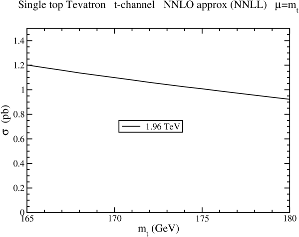
In Figure 2 we plot the approximate NNLO cross section from NNLL resummation for $t$-channel single top production at the Tevatron with $\sqrt{S}=1.96$ TeV versus top quark mass in the range from 165 to 180 GeV.

NNLO approx single top $t$-channel cross section (pb)
$m_{t}$ (GeV)	Tevatron 1.96 TeV	LHC 7 TeV	LHC 14 TeV
170	1.10	42.9	154
171	1.08	42.5	153
172	1.06	42.1	152
173	1.04	41.7	151
174	1.02	41.4	150
175	1.01	41.0	148

Table 1: The single top quark $t$-channel production cross section in pb in $p\overline{p}$ collisions at the Tevatron with $\sqrt{S}=1.96$ TeV, and in $pp$ collisions at the LHC with $\sqrt{S}=7$ TeV and 14 TeV, with $\mu=m_{t}$ and using the MSTW2008 NNLO pdf [29]. The approximate NNLO results are shown at NNLL accuracy.

Table 1 shows the numerical values of the cross section in pb for top quark mass values from 170 to 175 GeV in 1 GeV mass increments. At Tevatron energy the NNLO soft-gluon corrections are positive and they increase the NLO cross section by 4%. We note that the Tevatron cross sections presented in this paper are around 10% smaller than those in [13]; that difference is mostly due to the new pdf used in this paper.

There are theoretical uncertainties associated with these values that arise from the dependence on the scale $\mu$ as well as from pdf errors. The scale uncertainty is most commonly estimated by varying the scale by a factor of two, i.e. between $m_{t}/2$ and $2m_{t}$. For the approximate NNLO cross section at NNLL at the Tevatron the scale uncertainty is +0.1% $-$1.8%.

The pdf uncertainty is calculated using the 40 different MSTW2008 NNLO eigensets as provided by MSTW at 90% confidence level (C.L.) [29], which provides a conservative estimate of pdf error. For $t$-channel single top quark production at the Tevatron this 90% C.L. pdf uncertainty is +6.0% $-$5.9%.

The best current value of the top quark mass is $173$ GeV [30]. For this top quark mass we write the $t$-channel single top quark cross section and its associated uncertainties expilicitly as

$$\sigma_{\rm t-ch}^{\rm top}(m_{t}=173\,{\rm GeV},\,\sqrt{S}=1.96\,{\rm TeV})=1.04^{+0.00}_{-0.02}\pm 0.06\;{\rm pb}$$ (3.1)

where the first uncertainty is from scale variation and the second is the pdf uncertainty.

4 Single top $t$-channel production at the LHC

We continue with $t$-channel single top quark production at the LHC and we present results at both 7 TeV and 14 TeV energies. We note that at the LHC the single top cross section is different from that for single antitop production. Here we study only single top, while in Section 5 we study single antitop production.

Figure 3: The approximate NNLO cross section for single top quark production at the LHC with $\sqrt{S}=7$ TeV and 14 TeV.

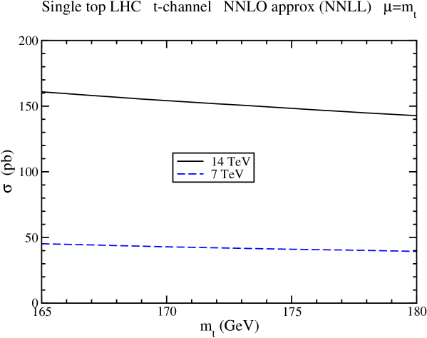
Figure 3 shows the approximate NNLO cross section from NNLL resummation for $t$-channel single top production at the LHC with $\sqrt{S}=7$ TeV and 14 TeV versus top quark mass in the range from 165 to 180 GeV. Table 1 shows the numerical values of the cross section in pb for both energy values for top quark masses from 170 to 175 GeV. At 7 TeV the NNLO soft-gluon corrections are negative and they decrease the NLO cross section by 1%; at 14 TeV they decrease it by 3%.

At 7 TeV the scale uncertainty is $+3.8$% $-0.5$% while the pdf uncertainty is $\pm 2.0$% at 90% C.L. For $m_{t}=173$ GeV we have

$$\sigma_{\rm t-ch}^{\rm top}(m_{t}=173\,{\rm GeV},\,\sqrt{S}=7\,{\rm TeV})=41.7^{+1.6}_{-0.2}\pm 0.8\;{\rm pb}$$ (4.1)

where the first uncertainty is from scale variation and the second from the pdf.

At 14 TeV the scale uncertainty is $+2.5$% $-0.6$% while the pdf uncertainty is +1.8% $-$2.2% at 90% C.L. For $m_{t}=173$ GeV we have

$$\sigma_{\rm t-ch}^{\rm top}(m_{t}=173\,{\rm GeV},\,\sqrt{S}=14\,{\rm TeV})=151^{+4}_{-1}\pm 3\;{\rm pb}$$ (4.2)

where the first uncertainty is from scale variation and the second from the pdf.

5 Single antitop $t$-channel production at the LHC

We continue with $t$-channel single antitop quark production at the LHC and we present results at both 7 TeV and 14 TeV energies.

Figure 4: The approximate NNLO cross section for single antitop production at the LHC with $\sqrt{S}=7$ TeV and 14 TeV.

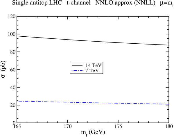
Figure 4 shows the approximate NNLO cross section from NNLL resummation for $t$-channel single antitop production at the LHC with $\sqrt{S}=7$ TeV and 14 TeV versus top quark mass in the range from 165 to 180 GeV.

NNLO approx single antitop $t$-channel cross section (pb)
$m_{t}$ (GeV)	LHC 7 TeV	LHC 14 TeV
170	23.2	93.8
171	23.0	93.0
172	22.8	92.3
173	22.5	91.6
174	22.3	91.0
175	22.1	90.3

Table 2: The single antitop $t$-channel production cross section in $pp$ collisions at the LHC with $\sqrt{S}=7$ TeV and 14 TeV, with $\mu=m_{t}$ and using the MSTW2008 NNLO pdf [29]. The approximate NNLO results are shown at NNLL accuracy.

Table 2 shows the numerical values of the antitop cross section in pb for both LHC energy values for top quark masses from 170 to 175 GeV in 1 GeV mass increments. At 7 TeV the NNLO soft-gluon corrections for single antitop production are negative and they decrease the NLO antitop cross section by 1%; at 14 TeV they decrease it by 3%. This is the same percentage contribution as we found for single top production in the previous section.

At 7 TeV the scale uncertainty is $+2.3$% $-2.1$% while the pdf uncertainty is $+3.0$% $-4.0$% at 90% C.L. For $m_{t}=173$ GeV we have

$$\sigma_{\rm t-ch}^{\rm antitop}(m_{t}=173\,{\rm GeV},\,\sqrt{S}=7\,{\rm TeV})=22.5\pm 0.5{}^{+0.7}_{-0.9}\;{\rm pb}$$ (5.1)

where the first uncertainty is from scale variation and the second from the pdf.

At 14 TeV the scale uncertainty is $+2.4$% $-1.0$% while the pdf uncertainty is +1.9% $-$3.2% at 90% C.L. For $m_{t}=173$ GeV we have

$$\sigma_{\rm t-ch}^{\rm antitop}(m_{t}=173\,{\rm GeV},\,\sqrt{S}=14\,{\rm TeV})=92{}^{+2}_{-1}{}^{+2}_{-3}\;{\rm pb}$$ (5.2)

where the first uncertainty is from scale variation and the second from the pdf.

By comparing Figs. 3 and 4, or Tables 1 and 2, we see that the single antitop cross section in the $t$ channel is 54% of that for single top at 7 TeV energy, while at 14 TeV it is 61% of that for single top production.

6 Conclusions and combinations of results for all channels

We have resummed collinear and soft gluon contributions to $t$-channel single top quark production at NNLL accuracy by using the two-loop soft anomalous dimension calculated in this paper. We have expanded the resummed cross section to NNLO and provided numerical studies of the cross section at Tevatron and LHC energies. These NNLO corrections are small for the $t$ channel, in contrast to the much larger contribution found in the $s$ channel in Ref. [17] and also for $tW$ (and $tH^{-}$) production found in Ref. [18].

We can now present combined results for the $t$ and $s$ channels at Tevatron and LHC energies for a top quark mass of 173 GeV. At the LHC the $tW$ cross section is also sizable.

For the Tevatron the sum of the cross sections in the $t$ and $s$ channels for single top production is $1.56^{+0.00}_{-0.02}\pm 0.09$ pb, where the first uncertainty is from scale variation and the second is from the pdf. The cross section is the same for single antitop production at the Tevatron.

For the LHC at 7 TeV the sum of the $t$ and $s$ channels for single top production is $44.9^{+1.6}_{-0.3}{}^{+1.0}_{-0.9}$ pb. For single antitop production the sum is $23.9\pm 0.5{}^{+0.7}_{-1.0}$ pb. In addition the $tW^{-}$ cross section is $7.8\pm 0.2{}^{+0.5}_{-0.6}$ pb, and for ${\bar{t}}W^{+}$ it is the same as that for $tW^{-}$.

For the LHC at 14 TeV the sum of the $t$ and $s$ channels for single top production is $159^{+4}_{-1}{}^{+3}_{-4}$ pb. For single antitop production the sum is $96{}^{+2}_{-1}{}^{+2}_{-3}$ pb. Also the $tW^{-}$ cross section is $41.8\pm 1.0{}^{+1.5}_{-2.4}$ pb, and the cross section for ${\bar{t}}W^{+}$ is the same.

References

- [1] D0 Collaboration, V.M. Abazov et al., Phys. Rev. Lett. 103, 092001 (2009) [arXiv:0903.0850 [hep-ex]]; Phys. Lett. B 682, 363 (2010) [arXiv:0907.4259 [hep-ex]]; Phys. Lett. B 690, 5 (2010) [arXiv:0912.1066 [hep-ex]].
- [2] CDF Collaboration, T. Aaltonen et al., Phys. Rev. Lett. 103, 092002 (2009) [arXiv:0903.0885 [hep-ex]]; Phys. Rev. D 82, 112005 (2010) [arXiv:1004.1181 [hep-ex]].
- [3] Tevatron Electroweak Working Group, arXiv:0908.2171v1 [hep-ex].
- [4] A.P. Heinson, Mod. Phys. Lett. A 25, 309 (2010) [arXiv:1002.4167 [hep-ex]]; A. Heinson and T.R. Junk, Ann. Rev. Nucl. Part. Sci. 61 (in press), arXiv:1101.1275 [hep-ex].
- [5] CMS Collaboration, V. Khachatryan et al., Phys. Lett. B 695, 424 (2011) [arXiv:1010.5994 [hep-ex]].
- [6] ATLAS Collaboration, G. Aad et al., arXiv:1012.1792 [hep-ex].
- [7] B.W. Harris, E. Laenen, L. Phaf, Z. Sullivan, and S. Weinzierl, Phys. Rev. D 66, 054024 (2002) [hep-ph/0207055].
- [8] J.M. Campbell, R. Frederix, F. Maltoni, and F. Tramontano, Phys. Rev. Lett. 102, 182003 (2009) [arXiv:0903.0005 [hep-ph]]; JHEP 10, 042 (2009) [arXiv:0907.3933 [hep-ph]].
- [9] P. Falgari, P. Mellor, and A. Signer, Phys. Rev. D 82, 054028 (2010) [arXiv:1007.0893 [hep-ph]].
- [10] R. Schwienhorst, C.-P. Yuan, C. Mueller, and Q.-H. Cao, Phys. Rev. D 83, 034019 (2011) [arXiv:1012.5132 [hep-ph]].
- [11] P. Falgari, F. Giannuzzi, P. Mellor, and A. Signer, arXiv:1102.5267 [hep-ph].
- [12] N. Kidonakis, JHEP 05, 011 (2005) [hep-ph/0412422].
- [13] N. Kidonakis, Phys. Rev. D 74, 114012 (2006) [hep-ph/0609287].
- [14] N. Kidonakis, Phys. Rev. D 75, 071501(R) (2007) [hep-ph/0701080].
- [15] S.M. Aybat, L.J. Dixon, and G. Sterman, Phys. Rev. Lett. 97, 072001 (2006) [hep-ph/0606254]; Phys. Rev. D 74, 074004 (2006) [hep-ph/0607309].
- [16] N. Kidonakis, Phys. Rev. Lett. 102, 232003 (2009) [arXiv:0903.2561 [hep-ph]]; eConf C090726, arXiv:0910.0473 [hep-ph].
- [17] N. Kidonakis, Phys. Rev. D 81, 054028 (2010) [arXiv:1001.5034 [hep-ph]].
- [18] N. Kidonakis, Phys.Rev. D 82, 054018 (2010) [arXiv:1005.4451 [hep-ph]].
- [19] N. Kidonakis, Phys. Rev. D 82, 114030 (2010) [arXiv:1009.4935 [hep-ph]].
- [20] H.X. Zhu, C.S. Li, J. Wang, and J.J. Zhang, JHEP 02, 099 (2011) [arXiv:1006.0681 [hep-ph]].
- [21] J. Wang, C.S. Li, H.X. Zhu, and J.J. Zhang, arXiv:1010.4509 [hep-ph].
- [22] N. Kidonakis and G. Sterman, Nucl. Phys. B 505, 321 (1997) [hep-ph/9705234].
- [23] G. Sterman, Nucl. Phys. B 281, 310 (1987).
- [24] S. Catani and L. Trentadue, Nucl. Phys. B 327, 323 (1989).
- [25] J. Kodaira and L. Trentadue, Phys. Lett. 112B, 66 (1982).
- [26] H. Contopanagos, E. Laenen, and G. Sterman, Nucl. Phys. B 484, 303 (1997) [hep-ph/9604313].
- [27] E. Laenen, G. Oderda, and G. Sterman, Phys. Lett. B 438, 173 (1998) [hep-ph/9806467].
- [28] N. Kidonakis and V. Del Duca, Phys. Lett. B 480, 87 (2000) [hep-ph/9911460].
- [29] A.D. Martin, W.J. Stirling, R.S. Thorne, and G. Watt, Eur. Phys. J. C 63, 189 (2009) [arXiv:0901.0002 [hep-ph]].
- [30] Tevatron Electroweak Working Group, arXiv:1007.3178 [hep-ex].