Top quark spin correlations at the Tevatron and the LHC

Abstract

Spin correlations of top quarks produced in hadron collisions have not been observed experimentally with large significance. In this Letter, we propose a new variable that may enable demonstration of the existence of spin correlations with $3-4~{}\sigma$ significance using just a few hundred dilepton events both at the Tevatron and the LHC. Such number of dilepton events has been observed at the Tevatron. At the LHC, it will become available once integrated luminosity of a few hundred inverse picobarns is collected.

The existence of spin correlations of top and anti-top quarks in $t\bar{t}$ pair production in hadron collisions is a solid prediction of the Standard Model. The possibility to observe these correlations is unique to top quarks since their large masses, short lifetimes and the relative weakness of chromomagnetic fields in the QCD vacuum, make it difficult for non-perturbative effects to depolarize $t$ and $\bar{t}$ before they decay. Therefore, if top quarks are produced in a particular polarization state, spin correlations can be observed by studying kinematic distributions of the top quark decay products which are sensitive to $t$ and $\bar{t}$ polarizations. For example, in the dilepton channel $pp(p\bar{p})\to t\bar{t}\to b\bar{b}\;l\bar{l}\;\nu\bar{\nu}$, the $V-A$ structure of the charged current forces momenta of anti-leptons (leptons) to be aligned (anti-aligned) with the direction of the top (anti-top) spin vectors.

The traditional way to study top quark spin correlations [1, 2, 3, 4, 5, 6, 7, 8, 9, 10] is fairly complex. It involves choosing the $t$ and $\bar{t}$ spin quantization axes and identifying suitable reference frames and angular distributions that are sensitive to these correlations. Because of the unobserved neutrinos in the dilepton events, full kinematics can not be reconstructed and determination of quantization axes and reference frames becomes difficult. This feature and a relatively low yield of dilepton events at the Tevatron is partially responsible for the fact that spin correlation measurements performed by the CDF and D0 collaborations are not conclusive. For example, the parameter $\kappa$ related to the top quark spin asymmetry in the dilepton channel at the Tevatron is predicted with a very small uncertainty in the Standard Model, $\kappa=0.78$ [1, 2, 3, 4, 6, 7, 8, 9, 10]. However, it is measured to be $\kappa=0.1^{+0.45}_{-0.45}$ and $\kappa=0.3^{+0.6}_{-0.8}$ by D0 [11] and CDF [12] collaborations, respectively, with $5.4(3.0)~{}{\rm fb}^{-1}$ of integrated luminosity. Although these results are consistent with the Standard Model, they do not demonstrate the existence of top quark spin correlations with sufficient significance. A similar situation occurs when spin correlations are measured in the lepton plus jets channel [13].

It is then natural to ask if a better way exists to establish the presence of spin correlations convincingly. This question was recently discussed by G. Mahlon and S. Parke in Ref. [14]. They suggested that spin correlations at the LHC can be observed by measuring the relative azimuthal angle $\Delta\phi$ of the two leptons from top decays in the laboratory frame, provided that only events with the low invariant mass of $t\bar{t}$ pairs, $M_{t\bar{t}}<400~{}{\rm GeV}$, are accepted. While in this case it is possible to distinguish spin-correlated and spin-uncorrelated events, Ref. [14] recognizes that placing a cut on $M_{t\bar{t}}$ is unphysical since, in dilepton events, the $t\bar{t}$ invariant mass can not be fully reconstructed on an event-by-event basis. Ref. [14] suggests that one can put a cut on the statistically reconstructed invariant mass $M_{t\bar{t}}$ but this cut does not seem to work as well as the cut on $M_{t\bar{t}}$ proper. It was later shown in Refs. [15, 16] that simpler cuts on kinematics of final state particles – for example an upper cut on the transverse momentum of the charged leptons – lead to the $\Delta\phi$ laboratory frame distributions that are sufficiently different to enable distinguishing between spin-correlations and no-spin-correlations hypotheses.

While Ref. [14] opened up a new direction in the studies of top quark spin correlations, similar to previous papers on the subject [1, 2, 3, 4, 5, 6, 7, 8, 9, 10] it focused on a single kinematic distribution. However, since many kinematic features of a particular event may be sensitive to top quark spin correlations, we should try to use all the information present in a particular event to establish their existence. To that end, we ask if, given a set of $t\bar{t}$ events observed at the Tevatron or the LHC, it is possible to distinguish the hypothesis that spins of the $t\bar{t}$ pair, entangled in the production process, remain entangled at the time of their decay, from the hypothesis that strong QCD dynamics depolarizes produced top quarks and kinematic features of their decay products are not correlated.

It is well-understood by now that the optimal way to answer this question requires the construction of a likelihood function, where the optimality should be understood in the sense of Neyman-Pearson lemma [17]. In our case, this lemma explains how to minimize the probability to accept the spin-correlation hypothesis when it is false, for fixed probability to reject spin-correlation hypothesis when it is true. We discuss how to construct the likelihood function. However, before going into this, we point out that we do not consider issues of experimental resolution in this Letter. In reality, experimental resolution may be important, so our results should be considered as the estimate of the highest significance with which two hypotheses can be separated.

We study dilepton events that contain two neutrinos in the final state, $pp(p\bar{p})\to t\bar{t}\to b\bar{b}\;l_{1}\bar{l}_{2}\;\bar{\nu}_{l_{1}}\bar{\nu}_{l_{2}}$. Because neutrino momenta can not be measured, the number of measurable kinematic variables ${{\mbox{\boldmath$x$}}}_{\rm obs}$ is smaller than the number of kinematic variables ${{\mbox{\boldmath$x$}}}=({{\mbox{\boldmath$x$}}}_{\rm obs},{{\mbox{\boldmath$x$}}}_{\rm unobs})$ needed to describe a particular event. The probability distribution for events with ${{\mbox{\boldmath$x$}}}_{\rm obs}$ set to a particular value is computed by integrating differential cross-sections for a hypothesis $H$ over unobserved kinematic variables. We write

$$P_{H}({{\mbox{\boldmath$x$}}}_{\rm obs})={\cal N}^{-1}_{H}\int{\rm d}{{\mbox{\boldmath$x$}}}_{\rm unobs}\frac{{\rm d}\sigma_{H}^{(0)}({\mbox{\boldmath$x$}})}{{\rm d}{{\mbox{\boldmath$x$}}}},$$ (1)

where ${\cal N}_{H}$ is the normalization factor. Given the two hypotheses, that the top quarks spins are correlated ($H=c$) or uncorrelated ($H=u$), we introduce a variable, related to a likelihood ratio for a single event, that emphasizes the difference between the two hypotheses

$${\cal R}({{\mbox{\boldmath$x$}}}_{\rm obs})=\frac{P_{c}({{\mbox{\boldmath$x$}}}_{\rm obs})}{P_{c}({{\mbox{\boldmath$x$}}}_{\rm obs})+P_{u}({{\mbox{\boldmath$x$}}}_{\rm obs})}.$$ (2)

We then calculate the probability distribution of the likelihood variable ${\cal R}({{\mbox{\boldmath$x$}}}_{\rm obs})$, given a particular hypothesis about the underlying physics

$$\rho_{H}({\cal R})=\sigma_{H}^{-1}\int{\rm d}{{\mbox{\boldmath$x$}}}\frac{{\rm d}\sigma_{H}({{\mbox{\boldmath$x$}}})}{{\rm d}{{\mbox{\boldmath$x$}}}}\delta({\cal R}({{\mbox{\boldmath$x$}}})-{\cal R}),$$ (3)

and perform statistical tests to see how many events are required to achieve the separation of the two hypotheses $H=c,u$.

It is important to realize that, at the expense of claiming that our likelihood ratio ${\cal R}$ is the optimal observable [18] to separate spin-correlation and no-spin-correlation hypotheses, we can use different cross-sections to construct the likelihood variable ${\cal R}({{\mbox{\boldmath$x$}}})$ in Eqs.(1,2) and to calculate the probability distribution $\rho_{H}({\cal R})$ in Eq.(3). We note that we use the Born differential cross-section ${\rm d}\sigma_{H}^{(0)}({{\mbox{\boldmath$x$}}})$ to define ${\cal R}({\bf x})$. This is a good choice because ${\rm d}\sigma_{H}^{(0)}({{\mbox{\boldmath$x$}}})$ captures main kinematic features of the actual physical process and it is inexpensive computationally. However, since this choice does not correspond to the actual probability distribution of the dilepton events, strictly speaking, ${\cal R}$ is not the optimal variable. Nevertheless, as long as ${\cal R}$ helps to separate the two hypotheses, optimality is not essential. We emphasize, however, that we use the best available approximation to the true cross-section ${\rm d}\sigma_{H}({{\mbox{\boldmath$x$}}})$ to construct the realistic probability distribution of the variable ${\cal R}$. To this end, in this Letter we employ the next-to-leading order (NLO) QCD prediction for the top pair production ${\rm d}\sigma_{t\bar{t}}$ that includes top quark spin correlations and radiative corrections to top quark decays [19].

Figure 1: Normalized distributions of the likelihood variable $R$ for the spin-correlation and no-spin-correlation hypotheses at the $7~{}{\rm TeV}$ LHC. The NLO QCD results for the distributions are shown. The bands correspond to the choices of the renormalization/factorization scales $0.5\;m_{t}<\mu<2m_{t}$.

Since we use the leading order cross-section to compute ${\cal R}$, the following issue appears. In general, the NLO QCD approximation includes processes with additional massless particles in the final state. Therefore, we need a prescription of how to map the kinematic features of such final states onto leading order kinematics. Indeed, at leading order the process $pp(p\bar{p})\to t\bar{t}\to b\bar{b}\;l\bar{l}\;\nu_{l}\bar{\nu}_{l}$ has two massless $b$-quarks. Associating these $b$-quarks with two $b$-jets reconstructed according to a well-defined jet algorithm solves the problem of additional radiation in the event. However, perturbatively, $b$-jets at leading order are massless, while this is not necessarily true in higher orders. This feature makes it difficult to connect the leading order kinematics that enters the calculation of ${\cal R}$ with kinematics of the actual event. To address this problem, we adopt the Ellis-Soper jet algorithm [20], where reconstructed jets are always massless.

Figure 2: Normalized distributions of the likelihood variable $R$ for the spin-correlation and no-spin-correlation hypotheses at the Tevatron. The NLO QCD results for the distributions are shown. The bands correspond to the choices of the renormalization/factorization scales $0.5\;m_{t}<\mu<2m_{t}$.

The discussion in the previous paragraph tells us how to map kinematics of a higher-order process to the kinematics of a tree-level process. As input for the calculation of the likelihood ${\cal R}({{\mbox{\boldmath$x$}}}_{\rm obs})$, we use four-momenta of the two $b$-jets, the four-momenta of the two charged leptons and the missing transverse momentum, which we identify with the component of the momentum of the two neutrinos, orthogonal to the collision axis. We also note that, since charges of $b$-jets can not be unambiguously defined, we require a procedure to assign one jet to be a $b$-quark jet and the other jet to be a $\bar{b}$-quark jet. We do this by computing the invariant mass of the positively charged lepton and the two $b$-jets and identifying the jet that minimizes this invariant mass, with the $b$-quark jet. The other $b$-jet is then identified with the $\bar{b}$-quark jet and, in leading order kinematics, we treat this jet as if it comes from the decay of the anti-top quark.

Having discussed a procedure to identify the input, we turn to the calculation of ${\cal R}$; this requires an integration of the tree-level differential cross-section for $pp(p\bar{p})\to t\bar{t}\to b\bar{b}\;l\bar{l}\;\nu_{l}\bar{\nu}_{l}$ over unobserved components of the neutrino momentum. In general this is difficult, but we assume that the process goes through the on-shell intermediate states, so that the invariant masses of $b\bar{l}\nu$ and $\bar{b}l\bar{\nu}$ are equal to $m_{t}$ and that the invariant masses of $\bar{l}\nu$ and $l\bar{\nu}$ are equal to $m_{W}$. Hence, we compute

$$\begin{split}&P_{H}(p_{\rm obs},p_{\perp,\rm miss})={\cal N}^{-1}_{H}\int[{\rm d}p_{\nu}][{\rm d}p_{\bar{\nu}}]\\ &\times\sum\limits_{ij}f_{i}(x_{1})f_{j}(x_{2})|{\cal M}_{H}^{ij}(p_{\rm obs},p_{\nu},p_{\bar{\nu}})|^{2}\\ &\times\delta^{(2)}({\mbox{\boldmath$p$}}_{\nu,\perp}+{\mbox{\boldmath$p$}}_{\bar{\nu},\perp}-{\mbox{\boldmath$p$}}_{\perp,\rm miss})\\ &\times\delta(M_{\bar{l}\nu}^{2}-m_{W}^{2})\delta(M_{l\bar{\nu}}^{2}-m_{W}^{2})\\ &\times\delta(M_{\bar{l}\nu b}^{2}-m_{t}^{2})\delta(M_{l\bar{\nu}\bar{b}}^{2}-m_{t}^{2}),\end{split}$$ (4)

where $[{\rm d}p]={\rm d}^{3}{\mbox{\boldmath$p$}}/((2\pi)^{3}2E)$ is the invariant integration measure, $p_{\rm obs}=\{p_{b},p_{\bar{b}},p_{l},p_{\bar{l}}\}$ is the set of observable momenta, $f_{i}(x)$ are parton distribution functions and $M_{ij..k}^{2}=(p_{i}+p_{j}+..+p_{k})^{2}$ are the respective invariant masses squared. As we see, there are six $\delta$-functions in Eq.(4), so that all integration variables are fixed; all we need to do is to solve the on-shell constraints. This is a standard procedure which is described e.g. in Ref. [21]; we do not repeat such a discussion here. In general, solving the on-shell constraints leads to several solutions (the maximal number is four), in which case all these solutions should be taken into account.

The result for the probability distribution reads

$$\begin{split}&P_{H}(p_{\rm obs},p_{\perp,{\rm miss}})={\cal N}^{-1}_{H}\sum_{ij}\sum\limits_{a}J_{a}\\ &\times f_{i}^{(a)}f_{j}^{(a)}|{\cal M}_{H}^{ij,\rm LO}(p_{\rm obs},p_{\nu}^{(a)},p_{\bar{\nu}}^{(a)})|^{2},\end{split}$$ (5)

where the second sum is over all the solutions that are obtained by reconstructing the final state and $J_{a}$ is the Jacobian which appears when the integration over the neutrino momentum is carried out. Also, $f_{i,j}^{(a)}=f_{i}(x_{1,2}^{(a)})$ is a parton distribution whose argument is reconstructed from the kinematics of a final state. Finally, we emphasize that in the calculation of probability distributions $P_{H}$ and the variable ${\cal R}$, we always use leading order matrix elements, as explicitly shown in Eq.(5).

The result for $P_{H}$ in Eq.(5) allows us to calculate the likelihood ${\cal R}$ and carry out the indicated program. In practice, however, we make use of the fact that both at the Tevatron and the LHC there is a single partonic channel that dominates the production process. Therefore, in Eq.(5), we use $i=(u,d),\;j=(\bar{u},\bar{d})$ to compute ${\cal R}$ for the Tevatron and $i=j=g$ to compute ${\cal R}$ for the LHC. We also neglect the dependence of the normalization factor ${\cal N}_{H}$ on the hypothesis $H$, following the observation that total cross-sections for $t\bar{t}$ pair production are insensitive to the (non)existence of top quark spin correlations. Finally, in the computation of the likelihood variable ${\cal R}({{\mbox{\boldmath$x$}}}_{\rm obs})$, we always set the renormalization and factorization scale to $m_{t}$ and use leading order parton distribution functions.

To calculate the probability distribution of the variable ${\cal R}$ for a given hypothesis $H$, we perform a numerical integration in Eq.(3). We generate events assuming that they must pass basic selection cuts for the $t\bar{t}$ events. For both the LHC and the Tevatron, we require $p_{\perp}^{l}>20~{}{\rm GeV}$, $p_{\perp}^{\rm miss}>40~{}{\rm GeV}$ and $|\eta_{l}|<2.5$. We also require that there are at least two $b$-jets in the event; jets are defined using Ellis-Soper jet algorithm [20] with $\Delta R=\sqrt{\Delta\eta^{2}+\Delta\phi^{2}}=0.4$ and the jet $p_{\perp}$-cut is set to $25~{}{\rm GeV}$ for both the Tevatron and the LHC. We use MRST2001 and MRST2004 parton distribution functions [22] in LO and NLO computations, respectively. All calculations that we report in this paper make use of the numerical program for computing NLO QCD effects in $t\bar{t}$ pair production, developed in Ref. [19].

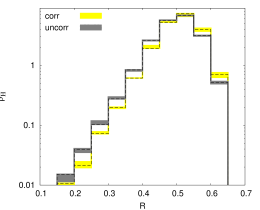
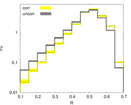
We now present the results of the calculation. First, we compute the distribution of the likelihood variable ${\cal R}$ for both spin-correlations and for no-spin-correlations hypotheses. These distributions are shown in Figs.1,2 for the LHC and the Tevatron, respectively. The two distributions are similar although the LHC distribution is more narrow. Also, as follows from Figs.1,2 the scale dependence of ${\cal R}$-distributions is small and we neglect it in what follows.

For both the Tevatron and the LHC, there is a difference between the two distributions, which is especially visible in the region of small ${\cal R}$. To find the number of events that is required to distinguish between the two ${\cal R}$ distributions, we perform a statistical test [23]. To this end, we generate $N$ events according to the probability distribution $\rho_{H}({\cal R})$ defined in Eq.(3) and calculate the quantity

$$L=2\;\ln[{\cal L}_{c}/{\cal L}_{u}],$$ (6)

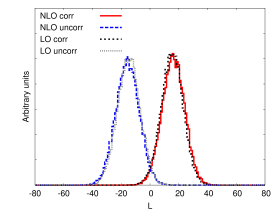
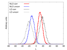
where ${\cal L}_{K}=\prod\limits_{i=1}^{N}\rho_{K}(R_{i})$. The statistical interpretation of $L$ can be found in Ref. [23]. We repeat this procedure multiple times, for $H=c,u$ and obtain two distributions of the variable $L$. The distribution of the variable $L$ is peaked at positive (negative) values if events are generated with the hypothesis $H=c$ ($H=u$) since, on average, ${\cal L}_{c}>{\cal L}_{u}$ (${\cal L}_{u}>{\cal L}_{c}$). Examples of such distributions are shown in Figs.3,4. To compute the significance $S$ with which the hypotheses $H=c$ and $H=u$ can be separated, we find the point beyond which the right-side tail of the left histogram and the left-side tail of the right histogram have equal areas. These areas correspond to the one-sided Gaussian probability outside of the $S/2\sigma$ range. If the two $L$-distributions are Gaussian with unit widths, the significance $S$ is the separation between peaks of the two distributions.

Figure 3: Distributions of the likelihood ratio for correct/false hypotheses, assuming five hundred dilepton events at the $7~{}{\rm TeV}$ LHC. Arbitrary units. We show LO and NLO QCD results for the $L$-distribution computed with $\mu=m_{t}$.

Figure 4: Distributions of the likelihood ratio for correct/false hypotheses, assuming three hundred dilepton events at the Tevatron. Arbitrary units. We show LO and NLO QCD predictions for the $L$-distribution computed with $\mu=m_{t}$.

The significance with which two hypotheses can be separated depends on the number of events $N$ with which the two hypotheses are probed. To understand what is a reasonable value of $N$, we note that the $pp\to t\bar{t}$ production cross-section at the $\sqrt{s}=7~{}{\rm TeV}$ LHC is approximately $160~{}{\rm pb}$ [24, 25]. Since $W$-bosons decay to electrons and muons twenty percent of the time, and assuming thirty percent efficiency, we find that $1~{}{\rm fb}^{-1}$ of the integrated luminosity corresponds, roughly, to $2500$ dilepton events. It is expected that $1~{}{\rm fb}^{-1}$ of luminosity will be collected at the LHC by the end of 2011 and this sets reasonable upper bound on the number of leptons $N$.

In fact, we do not need that many. We take $N=500$, which corresponds to $200~{}{\rm pb}^{-1}$, assuming $30\%$ efficiency. We then consider $10^{6}$ pseudo-experiments and obtain the two distributions shown in Fig.3. We convert the overlap of the two distributions into statistical significance and find that, with $500$ events, the two distributions shown in Fig.1 can be separated at the $4\sigma$ level. It is interesting to note that the difference between NLO and LO $L$-distributions at the LHC is very small, cf. Fig.3.

We now turn to the discussion of the $t\bar{t}$ production at the Tevatron. The production cross-section of the $t\bar{t}$ pairs at the Tevatron is, approximately, $7~{}{\rm pb}$ (for the latest measurements, see Refs. [26, 27]). Taking the accumulated luminosity to be $6~{}{\rm fb}^{-1}$ and assuming $30\%$ efficiency, we find that five hundred dilepton ($\mu,e$) events at the Tevatron should have been observed. We take $N=300$ and, by considering $10^{6}$ pseudoexperiments, we obtain $L$-distributions shown in Fig.4. In this case, there are significant differences between $L$-distributions computed at leading and next-to-leading order. Analyzing the $L$-distribution obtained with the NLO QCD approximation, we find that, with $300$ Tevatron dilepton events, the spin-correlation hypothesis can be established with the significance that is close to $3.5\sigma$.

Summary: We have shown that a likelihood-based analysis should make it possible to demonstrate the existence of top quark spin correlations in dilepton events at the Tevatron and the LHC. We constructed the relevant likelihood function and computed its probability distribution through next-to-leading order in perturbative QCD. Neglecting all the experimental uncertainties and the background contributions that are relatively small for the dilepton channel, we find that with $500$ dilepton events at the LHC and with $300$ dilepton events at the Tevatron the existence of spin correlations can be established with better than $3\sigma$ significance. This number of events will require just about $200~{}{\rm pb}^{-1}$ accumulated luminosity at the LHC and is already available at the Tevatron. We believe that our results are sufficiently encouraging to warrant a more complete study including proper treatment of experimental uncertainties and backgrounds.

Acknowledgments We are grateful to A. Gritsan for explaining to us the power of statistical methods. We acknowledge conversations with S. Parke that triggered our interest in physics of top quark spin correlations. We are indebted to A. Grohsjean, S. Parke and Y. Peters for discussions and for pointing out an error in the preliminary version of this paper. This research is supported by the NSF under grant PHY-0855365 and by the start-up funds provided by the Johns Hopkins University. Calculations reported in this paper were performed at the Homewood High Performance Cluster of the Johns Hopkins University.

References

- [1] G. Mahlon and S. J. Parke, Phys. Rev. D 53, 4886 (1996).
- [2] T. Stelzer and S. Willenbrock, Phys. Lett. B 374, 169 (1996).
- [3] A. Brandenburg, Phys. Lett. B 388, 626 (1996).
- [4] S. J. Parke and Y. Shadmi, Phys. Lett. B 387, 199 (1996).
- [5] K. Cheung, Phys. Rev. D55 (1997) 4430-4434.
- [6] G. Mahlon and S. J. Parke, Phys. Lett. B 411, 173 (1997).
- [7] W. Bernreuther, A. Brandenburg and Z. G. Si, Phys. Lett. B 483, 99 (2000).
- [8] W. Bernreuther, A. Brandenburg, Z. G. Si and P. Uwer, Phys. Lett. B 509, 53 (2001).
- [9] W. Bernreuther, A. Brandenburg, Z. G. Si and P. Uwer, Phys. Rev. Lett. 87, 242002 (2001).
- [10] W. Bernreuther, A. Brandenburg, Z. G. Si and P. Uwer, Nucl. Phys. B 690, 81 (2004).
- [11] V.M. Abazov, et al. [ D0 Collaboration ], [arXiv:1103.1871 [hep-ex]].
- [12] CDF collaboration, CDF note 9824 (2009).
- [13] T. Aaltonen et al. [ CDF Collaboration ], Phys. Rev. D83, 031104 (2011).
- [14] G. Mahlon and S. J. Parke, Phys. Rev. D 81, 074024 (2010).
- [15] M. Schulze, talk given at the LoopFest 2010 conference.
- [16] J. M. Campbell, R. K. Ellis, Nucl. Phys. Proc. Suppl. 205-206, 10-15 (2010). [arXiv:1007.3492 [hep-ph]].
- [17] J. Neyman and E.S. Pearson, Phil. Trans. R. Soc. Series A231, 289 (1993).
- [18] K. Cranmer and T. Plehn, Eur. Phys. J. C 51, 415 (2007).
- [19] K. Melnikov and M. Schulze, JHEP 0908:049 (2009).
- [20] S.D. Ellis and D.E. Soper, Phys. Rev. D 48, 3160 (1993).
- [21] L. Sonnenschein, Phys. Rev. D 73, 054015 (2006) [Erratum-ibid. D 78, 079902 (2008)].
- [22] A.D. Martin, R.G. Roberts, W.J. Stirling and R.S. Thorne, Phys. Lett. B 604, 61 (2004).
- [23] R. Cousins, J. Mumford, J. Tucker and V. Valuev, JHEP 11, 046 (2005).
- [24] V. Khachatryan et al. [ CMS Collaboration ], Phys. Lett. B 695 , 424 (2011).
- [25] G. Aad et al. [ Atlas Collaboration ], arXiv:1012.1792 [hep-ex].
- [26] V. M. Abazov et al. [ D0 Collaboration ], arXiv:1101.0124 [hep-ex].
- [27] T. Aaltonen et al. [ The CDF Collaboration ], Phys. Rev. D 82 , 052002 (2010).