Induced Delocalization by Correlation and Interaction
in the one-dimensional Anderson Model

Abstract

We consider long-range correlated disorder and mutual interacting particles according to a dipole–dipole coupling as modifications to the one-dimensional Anderson model. Technically we rely on the (numerical) exact diagonalization of the system’s Hamilitonian. From the perspective of different localization measures we confirm and extend the picture of the emergence of delocalized states with increasing correlations. Besides these studies a definition for multi-particle localization is proposed. In the case of two interacting bosons we observe a sensitivity of localization with respect to the range of the particle–particle interaction and insensitivity to the coupling’s sign, which should stimulate new theoretical approaches and experimental investigations with e.g. dipolar cold quantum gases.

I Introduction & Motivation

When P. W. Anderson introduced a simple quantum model to represent a disordered lattice Anderson (1958) it turned out that the contained physics is surprisingly complex, i.e. there exists the phenomenon of Anderson localization which is related to an exponential decay of the quantum mechanical probability distribution. A specific subclass of Hamiltonians Anderson studied reads

$$H_{s}=\sum^{L}_{i=1}{\epsilon_{i}c^{+}_{i}c_{i}}+J\sum^{L-1}_{i=1}{c^{+}_{i}c_{i+1}}+h.c.\quad,$$ (1)

which represents a single particle in a one-dimensional chain of $L$ sites with random (onsite) potential $\epsilon_{i}$ and kinetic energy $J$ (hopping energy). We assume the formalism of second quantization where the operator $c_{i}^{(+)}$ annihilates (creates) a boson at site $i$ and hence we refer to Eq. (1) as the disordered Bose–Hubbard model (without mutual interaction). One can either derive $H_{s}$ from the tight binding approximation of a continuous model Altland and Simons (2010) of non-interacting particles in an external potential or one ab initio takes it as a discrete model.

Based on the renormalization group flow idea one can argue that the conductance of a disordered solid may vanish for sufficient large systems Abrahams et al. (1979). In particular the one-dimensional disordered system, Eq. (1), becomes an insulator in the limit $L\to\infty$.

An explicit argument for localization of all states $\left|E\right\rangle$ satisfying $H_{s}\left|E\right\rangle=E\left|E\right\rangle$ can be established by exploiting the transfer matrix method Haake (2004) and a theorem due to Fürstenberg Fürstenberg (1963). On the other hand there is Bloch’s theorem Bloch (1928) which induces periodic (delocalized) states for a periodic lattice potential $\epsilon_{i}$. Hence the random nature of the potential must be obviously the key feature that leads to localization: A criterion based on the differentiability of the disorder potential $\epsilon_{i}$ was recently studied to understand the degree of randomness necessary for delocalization García-García and Cuevas (2009).

In order to investigate the impact of correlation on localization we introduce a specific disorder model that extrapolates from a pure random sequence $\epsilon_{1},\epsilon_{2},\dots,\epsilon_{L}$ to a periodic, and thus correlated, structure in Sect. II. It was first used by Moura & Lyra de Moura and Lyra (1998) and similar investigations followed Schubert et al. (2005); Kaya (2007). In a first step we will review the model on the basis of three different localization measures. Furthermore, we utilize one of those quantities to establish the phase diagram — namely, the dependence of localization with respect to disorder strength and the amount of correlation among the $\epsilon_{i}$. While a previous study by Shima et al.Shima et al. (2004) focused on the properties of states in the band center, our measure in use accounts for the global aspect, i.e. it incorporates properties of the entire spectrum.

The potential interest in the sensitivity of Anderson localization on correlated disorder arose due to recent experiments with Bose–Einstein condensates (BECs) where the direct observation of the atomic density distribution provides access to the quantum mechanical probability distribution Billy et al. (2008); Sanchez-Palencia and Lewenstein (2010). Besides correlation the impact of interaction is an issue one is naturally faced with when studying localization in BECs. Anderson already mentioned the importance of particle interaction Anderson (1978) on localization and worked out theoretical investigations in collaboration with L. Fleishman Fleishman and Anderson (1980). Over the years various aspects and features of interacting particles in a random potential have been figured out, but the problem remains a challenging topic for present research since results from different approaches do not always coincide. Just recently, the phase diagram of the 3-dimensional disordered Bose–Hubbard model was established Gurarie et al. (2009).

In our discussion on interacting particles in the presence of a disordered onsite potential (Sect. III) we first want to focus on a suitable definition of multi-particle localization and then turn to the extension of Eq. (1), namely

$$H_{mp}=H_{s}+\sum_{i,j=1}^{L}U_{ij}c^{+}_{i}c^{+}_{j}c_{i}c_{j}\quad,$$ (2)

with a (two-body) interaction potential $U_{ij}$. We model interaction according to a magnetic dipole–dipole coupling obtained in BEC experiments with dipolar gases Griesmaier et al. (2005); Stuhler et al. (2005) which is beyond the standard treatment of the onsite interaction term $U_{0}\sum_{i}\hat{n}_{i}(\hat{n}_{i}-1)$ (with $\hat{n}_{i}\equiv c^{+}_{i}c_{i}$) present in the disordered Bose–Hubbard model. By explicitely diagonalizing $H_{mp}$ for two interacting bosons we explore the relevance of interaction (especially its range) for localization and discuss an interesting symmetry involving the sign of the interaction potential $U_{ij}$.

II Correlated Disorder

To model correlated disorder we use the following prescription for the onsite potential values $\epsilon_{i}$ in Eq. (1):

$$\epsilon_{i}=\sum_{k=1}^{N/2}{\left[\frac{2\pi k}{N}\right]^{-\alpha/2}\cos{\left(\frac{2\pi}{N}ki+\phi_{k}\right)}}\quad{\small\begin{cases}&\alpha\geq 0\\ &N\gg L\end{cases}}\quad.$$ (3)

Here, $\alpha$ denotes the correlation parameter, $\phi_{k}\in[0,2\pi)$ are $\frac{N}{2}$ uniformly distributed random phases and $N$ is a natural number that should be much larger than the number of lattice sites $L$. Roughly speaking, the $\epsilon_{i}$ ($i=1\dots L$) represent the discrete Fourier transform of $k^{-\alpha}$, i.e. an algebraic decaying power spectrum Osborne and Provenzale (1988). One is therefore used to refer to the $\epsilon_{i}$ as long-range correlated and indeed if we turn back to the continuum limit, we can argue that the $\epsilon_{j}$ are correlated according to an algebraic decay for $\alpha\in(0,1)$. The case $\alpha=0$ corresponds to almost uncorrelated disorder which is close to the perfect disorder Anderson assumed in his model. More details on properties of the $\epsilon_{i}$ from Eq. (3) are provided in App. A.1.

II.1 Localization Measures

In order to detect the localization–delocalization transition we introduce three different measures:
a) the Normalized Standard Deviation Moore (1973) (NSD)
b) the Inverse Participation Ratio Kramer and MacKinnon (1993) (IPR) and
c) the Nearest Neighbor Distribution Brody et al. (1981) (NND).
While the NSD and the IPR are derived from the spatial/site probability distribution

$$\psi^{2}_{E}(i)\equiv\left|\langle i|E\rangle\right|^{2}\text{with}~{}H_{s}\left|E\right\rangle=E\left|E\right\rangle~{}\text{and}~{}\left|i\right\rangle\equiv c^{+}_{i}\left|0\right\rangle,$$ (4)

where $c_{i}\left|0\right\rangle=0$, the NND depends on the spectral values $E$ only. Given a chain of $L$ sites we calculate

$$\text{NSD}(E)\equiv\frac{\left\langle i^{2}\right\rangle-\left\langle i\right\rangle^{2}}{(L^{2}-1)/12}$$ (5)

where $\left\langle.\right\rangle\equiv\left\langle E\left|.\right|E\right\rangle$ denotes the expectation value and hence the NSD derives the (spatial) variance of the lattice site index $i$ for some $\left|E\right\rangle$ with respect to the state $\left|\psi\right\rangle$ whose probability distribution is uniform on the lattice.

In the case of the IPR one quantifies the (inverse) number of sites where $\psi^{2}_{E}(i)$ significantly differs from zero. Since $\sum_{i=1}^{L}\psi^{2}_{E}(i)=1$ we state that

$$\text{IPR}(E)\equiv\sum_{i=1}^{L}\left[\psi^{2}_{E}(i)\right]^{2}\sim\frac{1}{\tilde{L}}$$ (6)

with $\tilde{L}$ defined as the number of sites that are occupied by $\left|E\right\rangle$. Indeed, we can convince ourselves that $\text{IPR}\sim 1$ and $\text{IPR}\sim L^{-1}\xrightarrow{L\to\infty}0$ for localized and delocalized states, respectively.

In contrast, the NND considers the spectral properties of $H_{s}$. More precisely, we evaluate fluctuations of level spacings around a local mean $\bar{s}_{n}$ by computing

$$s_{n}\equiv(E_{n+1}-E_{n})/\bar{s}_{n}~{}\text{with}~{}\bar{s}_{n}\equiv\frac{E_{n+1+\frac{m}{2}}-E_{n-\frac{m}{2}}}{m+1},$$ (7)

and deriving the distribution $P(s)$ of the nearest neighbor spacings $s_{n}$. Here, we labeled the spectral values according to $E_{1}\leq E_{2}\leq\dots\leq E_{L}$ and the division by $\bar{s}_{n}$ unfolds Haake (2004) the level spacings to relate different parts of the whole spectrum to each other. The procedure of unfolding is not unique Gómez et al. (2002) and $m$ is left as a free parameter that defines the notion of local. We choose it such that $m\ll L$ on the one hand and to include enough energy values for reasonable statistics on the other hand; in fact, we used $m\sim 20$ for $L\sim 10^{3}$.

The NND is not as obvious as the former measures Efetov (2004); Simons and Altshuler (1996). Intuitively, the argument works as follows: Taking two different energy eigenstates $\left|E\right\rangle,\left|E^{\prime}\right\rangle$ that do not significantly overlap (in site space) we assume them to be almost orthogonal, i.e. they are in some sense independent from each other (localized) and nothing prevents the corresponding energy values to be arbitrary close ($s\to 0$). But if the overlap increases (extended states) the levels start to repell: $E\neq E^{\prime}$. Quantities that are statistically independent exhibit a Poissonian distribution and thus the corresponding NND should be Feingold et al. (1985) $P(s)\sim e^{-s}$. In contrast, $P(0)=0$ is reasonable to expect for delocalized states.

II.2 Numerical Results

Figure 1: (color online) Energy–resolved plot of the localization length (LL) for different correlation parameter values $\alpha$ to compare our results from exact (numerical) diagonalization to investigations that use the transfer matrix method to obtain the Lyapunov exponent $\gamma$ (cf. Ref. [de Moura and Lyra, 1998], fig. 5). We used a system of $L=3500$ sites and averaged over $50$ disorder realizations. The inset (transparent to the main panel in the background) presents numerical data of LL(0) for different system sizes which underpins the reported delocalization transition around $\alpha=2$.

Turning back to Eq. (1) we rescale $H_{s}$ by $J$, i.e. $H_{s}\to J^{-1}H_{s}$, which does not alter the Hamiltonian’s eigenstates but multiplies the spectral values $E$ by a factor of $J^{-1}$. Since we restrict the $\epsilon_{i}$ to the (finite) interval $[-\frac{\Delta}{2},\frac{\Delta}{2}]$ we introduce the parameter

$$\kappa\equiv\Delta/J$$ (8)

that indicates the strength of disorder. Thus we are faced with a two–dimensional set of system parameters $(\alpha,\kappa)$ and, from the following as well as App. A.1, it becomes clear that increasing $\alpha$ corresponds to increasing correlations up to long-range correlated disorder. Moreover, since the NSD and the IPR only depend on $\left|E\right\rangle$, we rescale and shift the spectrum such that the rescaled values $E\to e$ obey $-0.5\leq e\leq 0.5$ when plotting these quantities resolved in energy.

To set the stage, we want to relate our numerical results to previously published ones. Since it is common practise to attempt localization by computing the Lyapunov exponent  Haake (2004), we establish an exponential fit to $\left|E\right\rangle$. More precisely, our numerics picks out the maximum $\psi^{2}_{E}(i_{0})$ and performs an exponential fit into the direction singled out by $\max(i_{0},L-i_{0})$. From $\psi^{2}_{E,fit}(i)\sim\exp{(-\gamma\left|i-i_{0}\right|})$ we extract $\gamma(E)$ and define the localization length

$$\text{LL}(E)\equiv\gamma^{-1}(E)/L\quad.$$ (9)

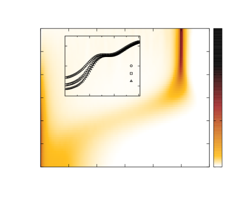
The corresponding result for intermediate disorder ($\kappa=1$) is shown in Fig. 1 and it exhibits reasonable qualitative agreement with Ref. [de Moura and Lyra, 1998], fig. 5; namely, delocalized states ($\gamma^{-1}\sim L\rightarrow\text{LL}\sim 1$) arise in a finite range around the band center $e=0$ when the correlation within the disorder potential $\epsilon_{i}$ is increased. This interpretation also coincides with the plot presented in Ref. [Schubert et al., 2005], fig. 3, where localization was quantified by means of a measure based on the density of states

$$\text{DOS}(E)\equiv\frac{dn}{dE}$$ (10)

which defines the number $dn$ of energy eigenstates $\left|E\right\rangle$ in a given interval $[E,E+dE]$.

Moreover, the work of Moura & Lyra mentioned above supports delocalization at $\alpha=2$ for states at the

Figure 2: (color online) Plot of the distribution $P(\text{NSD})$ of the (spatially) normalized standard deviation Eq. (5) at intermediate disorder $\kappa=1$ ($J=\Delta$) to support that localization$\to$delocalization takes place rather smoothly than according to a sharp transition. As for Fig. 1 we used $L=3500$ and the averaging was taken over $50$ disorder realizations. The inset (transparent to its background) shows results for different system sizes and supports our crossover picture as well (details in the main text).

band center. Therefore we depicted a cut of Fig. 1 at $e=0$ in the relevant correlation parameter range $\alpha\in[1,3]$ and checked $\text{LL}(0)$ according to a finite size analysis, inset of Fig. 1. Indeed, up to $\alpha\approx 2$ the $\text{LL}(0)$ decreases with increasing system size $L$ while above this correlation parameter value it remains relatively constant. Assuming that this trend persits for even larger system sizes, the data support that $\alpha=2$ marks a qualitative difference between systems with smaller and larger correlation, respectively: While the relative extend of the states with respect to the system size falls off (localization) for $0\leq\alpha\lesssim 2$, it remains constant (extended states) for $\alpha\gtrsim 2$ in the thermodynamic limit $L\to\infty$.

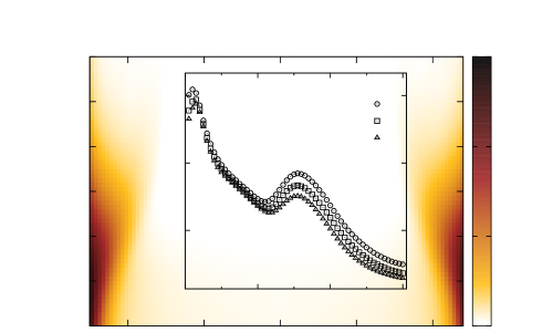
However, we would like to address the question where (in terms of $\alpha$) does the localization–delocalization transition takes place from the perspective of the measures introduced in Sect. II.1: Instead of a sharp transition at $\alpha=2$, which is supported by Fig. 1 and publications mentioned above, we suggest a smooth crossover in $1\lesssim\alpha\lesssim 2$. Investigating the distribution $P(\text{NSD})$ most obviously illustrates this statement and we present it in Fig. 2. Although the major fraction of localized states ($\text{NSD}\ll 1$) becomes delocalized at $\alpha\approx 2$ there is a finite fraction that splits apart the localized region ($0\leq\text{NSD}\lesssim 0.2$) around $\alpha=0.5$ and drifts

Figure 3: (color online) Smooth localization–delocalization crossover from the perspective of the simultaneous analysis of the IPR and the DOS. Increasing correlation attracts the system’s states from the band edges ($\left|e\right|=0.5$) to the band center ($e=0$) where delocalized states are present and thus the system becomes more and more delocalized. Finally, localized states almost completely vanish above $\alpha=2$. The inset of the upper panel (transparent to the background again) establishes the finite size analysis similar to the inset of Fig. 2.

towards the delocalized regime ($\text{NSD}\approx 1$) up to $\alpha\approx 2$. This observation remains stable in the numerically studied range of system sizes ($L=1000\dots 3500$).

An explicit plot to the finite size analysis performed with respect to our crossover picture is given by the inset of Fig. 2. Convoluting the NSD with the DOS, i.e.

$$\overline{\text{NSD}}\equiv\int dE~{}\text{NSD}(E)\text{DOS}(E)$$ (11)

yields a single quantity to characterize the global localization property of the disorderd system at fixed correlation parameter $\alpha$. In the spirit of the previously applied LL–dependence on $L$, the inset of Fig. 2 provides the system size dependence of the averaged normalized standard deviation $\overline{\text{NSD}}$: Up to $\alpha\approx 1$, $\overline{\text{NSD}}$ decreases with increasing system size $L$ indicating that the Hamiltonian’s eigenstates stay localized in the thermodynamic limit. Above $\alpha\approx 1$ the averaged standard deviation that is normalized to $L$ remains unaltered for the accessed number of sites — a signature of delocalization. Remarkably, the $\overline{\text{NSD}}$ forms a plateau in $1\lesssim\alpha\lesssim 2$, before growing up in absolute value with increasing correlation. One more evidence to the crossover picture we are in favor of.

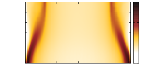
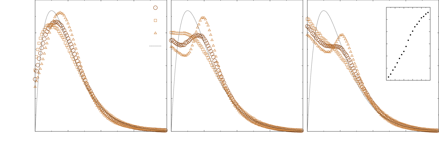
Similarly, we investigate the IPR taking into account the DOS from Eq. (10). Since we are interested in the localization property of the whole system it is necessary to account for the number of states with a certain localization measure value. Hence the IPR and the DOS are plotted simultaneously in Fig. 3 and the inset of the upper panel presents an averaged version of the inverse participation ratio in total analogy to Eq. (11) with $\text{NSD}(E)$ replaced by $\text{IPR}(E)$.

From a naive point of view we could conclude that even for weak correlation ($\alpha\lesssim 0.5$) the system is delocalized since there are only a few localized states near the band edges ($\left|e\right|=0.5$) while the rest of the spectrum exhibits an IPR value corresponding to delocalization. Moreover, increasing correlation enhances localization up to $\alpha\approx 1$ which seems unexpected. But if we include the DOS (lower panel of Fig. 3) the picture drawn before reveals: We realize that almost all states have energies near to the band edges for $\alpha\lesssim 0.5$ and thus the system is localized. The crucial fact leading to the localization–delocalization crossover is that for increasing correlation the band center attracts the states from the band edges to the regime where delocalized states are permanently present ($\left|e\right|\lesssim 0.3$). Localized states at the band edges follow that trend only up to $\alpha\approx 1$ and for stronger correlation they start to disappear until they are almost vanished at $\alpha\approx 2$. According to an argument presented in App. A.1 it is reasonable to refer to disorder with $\alpha\geq 1$ as highly correlated and therefore it provides a hint to the suggestive importance of $\alpha=1$ in our data.

Again, this observation is confirmed by a finite size analysis as shown in the inset of the upper panel of Fig. 3. We note that the $\overline{\text{IPR}}$–values stay quite unaltered for $\alpha\lesssim 1$ when $L$ is increased: Since $\text{IPR}\sim\tilde{L}^{-1}\sim L^{-1}$ (cf. Eq. 6) corresponds to extended states which tends to zero in the limit $L\to\infty$, the decreasing behavior of $\overline{\text{IPR}}(L)$ for $\alpha\gtrsim 1$ suggests the existence of delocalized states. The bump in the crossover interval $\alpha\in[1,2]$ may represent a finite size effect that eventually vanishes in the thermodynamic limit.

Finally, we would like to take a closer look at the smooth crossover from the perspective of the energy spectrum. Therefore we investigate the NND from Sect. II.1 which also prepares the relevant measure we will use to quantify the $(\kappa,\alpha)$–dependence of localization. Plots of the NND for different correlation parameters $\alpha$ are presented in Fig. 4. For small $\alpha$ the result is near to the Poissonian distribution $e^{-s}$. Deviations from the theoretical prediction are due to the finite system size $L$ and the fact that $\alpha=0$ does not exactly correspond to uncorrelated but weakly correlated disorder (see App. A.1). We further note that the data points for $\alpha=0$ and $\alpha=0.5$ almost coincide,

Figure 4: (color online) Semi-logarithmic plot of the nearest neighbor spacing distributions for several correlation parameter values $\alpha$ ($L=3\cdot 10^{4}$, $\kappa=1$). The broken line is to compare them to the Poissonian distribution $P_{\text{P}}$ which we expect for localized states. As apparent, the distribution does not converge to $P_{\text{WD}}$ of the Gaussian orthogonal ensembleHaake (2004) since for $\alpha\gg 1$ the onsite potential $\epsilon_{i}$ becomes periodic, local fluctuations among the $E_{i}$ vanish and thus $P(s)$ must be peaked around $s=1$ ($s_{n}=(E_{n+1}-E_{n})/\bar{s}_{n}\approx 1,~{}\alpha\gg 1$). A more detailed discussion is given in the main text.

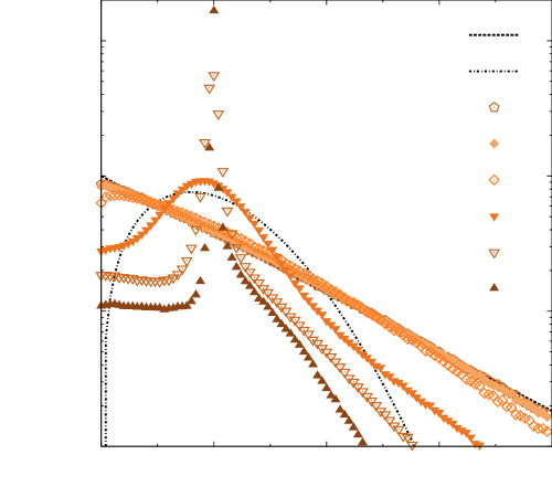
but when increasing $\alpha$ above $0.5$ the distribution starts to deviate more significantly from $e^{-s}$ to become peaked around $s=1$. Returning to Eq. (3) we note that for $\alpha\gg 1$ the summation over the (discrete) momenta $k$ picks up less cosine modes which leads to a periodic onsite potential in the limit $\alpha\to\infty$. Hence the spectrum of $H_{s}$ becomes more regular for increasing $\alpha$ and (local) fluctutations eventually vanish for sufficiently strong correlation due to Bloch’s theorem. From the definition of the unfolded level spacings $s_{n}$, Eq. (7), we conclude that all $s$ values should be centered around $1$ due to the normalization by the local mean $\bar{s}_{n}$.

At this stage it is maybe advisable to discuss the Wigner surmise $P_{\text{WD}}$ — a specific NND connected to random matrix theoryHaake (2004) — in the context of localization, especially in our specific model system under consideration. In the literatureShklovskii et al. (1993); Jacquod (1998); Cuevas (1999) it seems to be common practise to associate

$$P_{\text{P}}(s)\equiv\exp(-s)$$ (12)

with localized states and signatures of level repulsion ($P(s\ll 1)\ll 1$) in the NND with extended ones after having unfolded the spectrum of the corresponding disordered system. In the case of a time reversal symmetric quantum chaotic system — represented by real, symmetric random matrices — the NND adopts the Wigner surmise

$$P_{\text{WD}}(s)\equiv\frac{\pi}{2}s\exp\left(-\frac{\pi}{4}s^{2}\right)$$ (13)

in the thermodynamic limit (cf. Ref. Haake, 2004 as well as references therein).

As we scetched it in Sect. II.1 it is quite plausible to adopt the first correspondence. Indeed, the matrix representation of $H_{s}$ in the site basis $\{\left|i\right\rangle\}$ becomes tridiagonal, i.e.

$$H_{s,ij}\equiv\left\langle i\left|H_{s}\right|j\right\rangle$$ (14)

vanishes except for its diagonal elements $H_{s,ii}=\epsilon_{i}$ and the first off-diagonal entries $H_{s,ii+1}=H_{s,i+1i}=J$ when open boundary conditions (cf. App. A.2) are imposed. In the limit where the (uncorrelated) disorder strongly dominates the kinetic energy ($\Delta\gg J$), the single particle Hamiltonian becomes approximately diagonal to zeroth order in $\tfrac{J}{\Delta}$ and the solution to the Schrödinger equation reads $\left|E_{i}\right\rangle\approx\left|i\right\rangle$ with $E_{i}\approx\epsilon_{i}$. Hence the almost purely random/uncorrelated sequence of eigenvalues $E_{i}$ should obey a Poissonian distribution in the NND.

However, there is a crucial fact we would like to keep in mind: Although the Hamilton matrix of $H_{s}$ is real valued and symmetric (in site space) — since we deal with static disorder $\epsilon_{i}$ and real valued constant hopping energy $J$ — the elements $H_{s,ij}$ do not fulfill one of the conditions from which $P_{\text{WD}}$ is derived as the corresponding NND of quantum chaotic systems. Therefore we will not naturally expect the Wigner surmise to arise in the presence of delocalized states. Indeed, Fig. 4 numerically verifies this conjecture.

An issue closely related to the analysis of the NND is the question on a critical distribution $P_{c}$ that marks the transition from localization to delocalization. One way to detect this transition by means of the NND is to argue for a suitable intermediate distribution between $P_{\text{P}}$ and $P_{\text{WD}}$ as done in e.g. Ref. [Shklovskii et al., 1993]. Usually one investigates the quantity

$$\eta\equiv\frac{\int ds~{}[P(s)-P_{\text{WD}}(s)]}{\int ds~{}[P_{\text{P}}(s)-P_{\text{WD}}(s)]}$$ (15)

based on the NND $P(s)$ where the integrals may be chosen (including a proper argumentation) on a suitable interval where one expects sensitivity of $P(s)$ on localization. According to our discussion from Sect. II.1 one may take $s\in[0,s_{max}]$ with $s_{max}$ smaller than the smallest root of $P_{\text{WD}}(s)=P_{\text{P}}(s)$. But since our one-dimensional disordered system in use does not converge to the Wigner surmise it is rather vague to apply Eq. (15) in order to resolve the question on the impact of correlation on localization.

Nevertheless, the previous discussion invites us to introduce a similar measure for plotting the dependence of localization on the parameter space $(\alpha,\kappa)$ which will be the last purpose of this section on correlated disorder. We determine the deviation of $P(s)$ from $P_{\text{P}}$ as a quantity for the degree of delocalization. Thus we define

$$L^{2}_{\text{NND}}(\kappa,\alpha)\equiv s^{-1}_{\text{max}}\int_{0}^{s_{\text{max}}}ds[P(s,\kappa,\alpha)-P_{\text{P}}(s)]^{2}$$ (16)

where $s_{\text{max}}$ introduces the numerically necessary restriction to a finite range of $s$–values and we use $L_{\text{NND}}\equiv\sqrt{L^{2}_{\text{NND}}}$ as a localization measure. Numerically, $L_{\text{NND}}$ features the striking advantage that it is sufficient to just compute the eigenvalues of the Hamilton matrix $H_{s,ij}$ and therefore we are able to reach larger system sizes $L$ with our code.

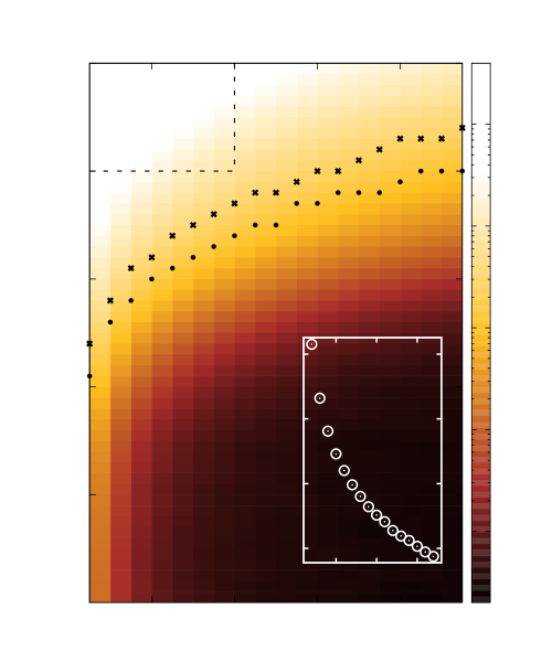
As we know from the previous considerations on the localization–delocalization crossover for intermediate disorder ($\kappa=1$, first part of Sect. II.2), correlation with $1\leq\alpha\leq 2$ seems to be important for delocalization; varying $\alpha$ in $[0,2.5]$ will cover it. In the limit $\kappa\to 0$, i.e. vanishing disorder, it is obviously hardly possible to recover Anderson’s result for infinitely extended systems and arbitrary small disorder, since we have to face the fact to be generally restricted to finite system sizes $L$ and finite numerical precision. Therefore we investigate the domain $(\alpha,\kappa)\in[0,2.5]\times[0.5,10]$ which spans a wide range of disorder strengths $\kappa$ for the interesting amount of correlation among the onsite disorder potential values $\epsilon_{i}$. The corresponding result is shown in Fig. 5

Figure 5: (color online) $(\kappa,\alpha)$–dependence of localization in the one-dimensional Anderson model from the perspective of a measure based on the nearest neighbor spacing distribution (NND) of the Hamiltonian’s spectrum with $L=3\cdot 10^{4}$. The finite size analysis with the measure $\Delta[L^{2}_{\text{NND}}]^{2}$, defined in Eq. (17), is shown as an inset (white). Furthermore we included the region which corresponds to extended states according to the work of Shima et al.Shima et al. (2004) who tackeled the phase diagram by means of states in the band center $E=0$ using the transfer matrix method. The ($\bullet$) mark the minimal deviation of the NND from $P_{\text{SP}}$ (cf. Eq. (18)) for fixed disorder strength $\kappa$ and the (x) indicate the same minima with respect to $P_{\text{WD}}$.

with $L=3\cdot 10^{4}$ and the inset presents the finite size analysis we performed: Let $\Delta L$ denote the (fixed) difference between two system sizes $L$ and $L^{\prime}$ such that $L=L^{\prime}+\Delta L$ and we define

$$\Delta[L^{2}_{\text{NND}}]^{2}(L,\Delta L)\equiv\left|\mathcal{A}\right|^{-1}\int_{\mathcal{A}}d\kappa d\alpha~{}\times\\ [L^{2}_{\text{NND}}(\kappa,\alpha,L)-L^{2}_{\text{NND}}(\kappa,\alpha,L^{\prime})]^{2}$$ (17)

with $\left|\mathcal{A}\right|=\left|[0,2.5]\times[0.5,10]\right|=\Delta\kappa\Delta\alpha$ the area of integration. The white inset plots that quantity versus $L$ having fixed $\Delta L=1000$; it becomes clear that Fig. 5 exhibits a convergent trend for increasing $L$.

Before turning to a more detailed analysis of $L_{\text{NND}}(\kappa,\alpha)$ let us come back to our comments on a critical distribution $P_{c}$. As stated before we do not expect the NND to converge to $P_{\text{WD}}$ in the limit $\alpha\to\infty$ (delocalized system). In our case it is not well justified to assume, e.g., the Semi-Poisson lawJacquod (1998)

$$P_{\text{SP}}(s)\equiv 4s\exp(-2s)$$ (18)

that resembles the linear increase of $P_{\text{WD}}(s)$ for $s\ll 1$ and an exponential decay for $s\gg 1$ to be critical. Numerical evidence on our claim provides Fig. 5 where we plot both the minimal deviation of the NND from $P_{\text{SP}}$ ($\bullet$) and $P_{\text{WD}}$ (x) for fixed disorder strength $\kappa$. The notion deviation is defined in total analogy to Eq. (16). In the case of the convergence of the NND to $P_{\text{WD}}$ we would expect the minima (x) to appear at the maximal $\alpha$–value simulated — independent from the disorder strength $\kappa$. But, as visible in Fig. 5, the NND passes by $P_{\text{WD}}$ below $\alpha\approx 2.2$. But surprisingly, the deviation minima of the NND from $P_{\text{SP}}$ ($\bullet$) appear to lie in the crossover region $1<\alpha<2$ we emphasized during our previous numerical studies. Moreover, they follow the qualitative trend of our localization measure $L_{\text{NND}}$ which one may naively exploit to argue in favor of $P_{\text{SP}}$ as a suitable critical distribution. But a closer look on the precise shape of the NND with minimal deviation from $P_{\text{SP}}$ reveals significant differences from the Semi-Poisson law that become even more obvious with increasing disorder strength $\kappa$. A corresponding plot is shown in Fig. 6. Therefore, we do not support the Semi-Poisson law $P_{\text{SP}}$ as a suitable critical distribution. In fact it is designed as a hybrid between the two limiting cases of a Poisson distribution $P_{\text{P}}$ and the Wigner surmise $P_{\text{WD}}$ which does not apply to extended states in our specific model.

Figure 6: (color online) NNDs for different disorder strengths $\kappa$ ($L=3\cdot 10^{4}$) to illustrate that the Semi-Poisson law $P_{\text{SP}}$ as a hybrid between the Poisson distribution $P_{\text{P}}$ and the Wigner surmise $P_{\text{WD}}$ is not an appropriate critical distribution to indicate delocalization for our model under consideration. The NND $P(s)$ with $\alpha_{\text{min}}$ ($\odot$) is singled out by its minimal deviation from $P_{\text{SP}}$ for fixed $\kappa$ as described in the main text (cf. also ($\bullet$) in Fig. 5). Plotting $P(s)$ with $\alpha_{\text{min}}\pm 0.1$ underlines the two statements we emphasized: a) decreasing values of the NND for $s\to 0$ (level repulsion) and b) development of a peak of $P(s)$ around $s=1$ for increasing correlation parameter $\alpha$ due extended states (increase of $P(1)$). The inset in the right panel shows the dependence of the minimal deviation from $P_{\text{SP}}$ with respect to the disorder strength.

However, there has been a similar investigation to our phase diagram in Ref. [Shima et al., 2004] and we would like to discuss some conclusions one may draw when comparing the two results now. Shima et al. report numerical studies that support the existence of extended states for $(\kappa,\alpha)\in[0,4]\times[2,5]$ on basis of a quantity $\Lambda$ similar to our LL evaluated at the band center $e=0$ (cf. their Fig. 6). We separated the corresponding region of extended states in Fig. 5 by a dashed line. There are two main differences we would like to point out with respect to our investigations of $L_{\text{NND}}(\kappa,\alpha)$: First of all, the localization–delocalization crossover depends on the disorder strength and second $L_{\text{NND}}$ varies over approximately two orders of magnitude in $1\lesssim\alpha\lesssim 2$ quite independently from the value $\kappa$. Therefore the evaluation of the NND underlines the picture of a smooth crossover between localization and delocalization drawn before. The qualitative result of delocalization for all $\kappa$–values under consideration is in accordance with our line of reasoning that the disordered system has to eventually delocalize for $\alpha\to\infty$ due to Bloch’s theorem. Therefore it would be interesting to push the numerical analysis of Shima et al. beyond their maximal correlation $\alpha\leftrightarrow p=5$. However, assuming that the deviation of the results of Shima et al. and our investigations is not caused by some hidden technicality, the discrepancy of our conclusions to Shima et al. may reveal two useful lessons:

1. It reminds us of the difficulty of a proper interpretation of the NND with respect to localization. The quantities $\Lambda$ and LL, respectively, are much closer to the original picture of localization drawn by P. W. Anderson and thus one may prefer it in cases where physical intuition is hard to gain. The NND always needs reasonable understanding of the system under examiniation.

2. While Shima et al. focused on the states in the band center of the disordered one-dimensional system, the NND indirectly takes into account the (averaged) localization property of all states. Assuming that both quantities properly account for localization, it seems that, at least for $(\kappa,\alpha)\in[4,8]\times[2,5]$, the properties of states with $E=0$ are not dominating enough to show up when all states are included.

As a closing remark we would like to note that the previous discussion points out that the application of the NND as a localization measure is not as straightforward as the other quantities in the particular system we are investigating. Even though its appealing property of being basis independent and thus easily employable for studying interacting particles, its interpretation remains complicated. Eventually, this observation prevents us from utilizing it in order to detect localization of multiple particles and we would rather like to argue for an intuitive observable in the section below.

III Localization in the Presence of Interaction

In this second part of our discussion on delocalization in the one-dimensional Anderson model we want to turn to the question how localization is effected by the presence of interaction. This problem basically goes beyond the scope of the quantum physics of $H_{s}$ originally encountered by Anderson, but — as mentioned in the beginning — the question of the impact of interaction already attracted his attention in the late 1970s. Nevertheless the problem has remained a challenging topic and experiments with BECs in optical lattices have re–raised the focus on it during the past few years.

With Eq. (2) at hand, namely

$$H_{mp}=\sum^{L}_{i=1}{\epsilon_{i}c^{+}_{i}c_{i}}+J\sum^{L-1}_{i=1}{c^{+}_{i}c_{i+1}}+\sum_{i,j=1}^{L}U_{ij}c^{+}_{i}c^{+}_{j}c_{i}c_{j}+h.c.~{},$$ (19)

we introduce an interaction term $U_{ij}c^{+}_{i}c^{+}_{j}c_{i}c_{j}$ where for $U_{ij}=U_{0}\delta_{ij}$ one encounters the disordered Bose–Hubbard model assuming bosonic commutation relations for the lattice site annihilation (creation) operators $c_{i}^{(+)}$. $U_{0}=const.$ describes contact/onsite interaction, i.e. particles interact only when occupying the same site. But as we will carry out in Sect. III.2 it is convenient to assume the more general case, Eq. (19), to describe experiments with either Rydberg gases Li et al. (2005); Singer et al. (2004) or (dipolar) BECs Griesmaier et al. (2005) where particles interact even if separated by a (large) number of lattice sites. In particular, we use an algebraic decaying interaction potential and therefore conceptually bridge from long-range correlation to long-range interaction.

III.1 Defining Localization

Before proceeding we have to deal with the question on how to treat localization for multiple (interacting) particles, since localization was originally defined for the single particle problem. The literature provides several approaches for a suitable definition. E.g. one can use the Hausdorff measure Aizenman and Warzel (2009) as a distance between two states $\psi_{0}$ and $\psi_{t}$ where the latter is the former one evolved in time by the Schrödinger equation $i\hbar\partial_{t}\left|\psi\right\rangle=H_{mp}\left|\psi\right\rangle$. In analogy to Anderson’s initiating paper Anderson (1958) one can then ask, roughly speaking, for the absence of diffusion in terms of that distance. Another idea is to relate localization to macroscopic observables and associate the notion of localization to vanishing electrical conductivity Basko et al. (2006). Furthermore one can directly study localization in Fock space as performed, e.g., in Ref. [Berkovits and Avishai, 1998]. An ansatz independent of the specific form of the Hamiltonian — and thus easily applicable to the interacting problem — is the analysis of spectral statistics (cf. Eq. (7)) Cuevas (1999) which is driven by the analogy between random matrices in quantum chaos and the random Hamilton matrices due to disorder. But as extensively discussed in Sect. II.2 its strength of being representation independent may come along with some difficulties due to a proper interpretation of the corresponding results. Furthermore, the application of the NND to systems of multi-particles shifts the argument of level repulsion given in Sect. II.1 to localization in Fock space.

For our purpose we want to propose a rather intuitive solution inspired by a quantity which seems to be natural under the scope of experiments with cold atoms and which is connected to the particle density. Therefore we try to motivate a projection of the many–particle state to the lattice sites $i=1\dots L$ and apply a one–particle localization measure afterwards. Of course, the procedure has to coincide with the notion of single particle localization if we return to a set of Fock states with one particle at a given site.

Since one is able to directly image the density profile of Bose–Einstein condensates in experiment Billy et al. (2008) we consider the question on the probability $p_{i}$ to find at least one particle at site $i$. Using the language of second quantization we define the projection operator

$$\mathcal{P}_{i}\equiv\frac{c_{i}}{\sqrt{n_{i}+\delta_{0n_{i}}}}$$ (20)

where $n_{i}$ is the eigenvalue of the number operator $\hat{n}_{i}\equiv c_{i}^{+}c_{i}$ counting the number of bosons at site $i$ and the Kronecker delta $\delta_{kl}$ ensures that $\mathcal{P}_{i}$ is well defined for $n_{i}=0$. Given an eigenstate $\left|E\right\rangle$ of $H_{mp}$ we can answer our question from above by

$$p_{i}(E)\propto\left|\left\langle E\right|(\mathcal{P}_{i}^{+}\mathcal{P}_{i})\left|E\right\rangle\right|^{2}$$ (21)

and the constant of proportionality is obtained by the normalization condition $1=\sum_{i=1}^{L}p_{i}$. Therefore we end up with a projection of the multi-particle state $\left|E\right\rangle$ onto the site basis $\left|i\right\rangle$ by the probability distribution $p_{i}(E)$. For the single particle problem this projection is exactly given by the site basis representation of $\left|E\right\rangle$, i.e. $p_{i}(E)=\left|\langle i|E\rangle\right|^{2}$ whose properties we studied for correlated disorder above. Hence the natural step to perform next is to apply the NSD or the IPR on $p_{i}$ ($i=1\dots L$). But there is an argument excluding the application of the NSD measure: Suppose, two particles are localized at certain sites $i_{1}$ and $i_{2}$, i.e. $p_{i}$ is peaked for $i\in\{i_{1},i_{2}\}$. If $\left|i_{1}-i_{2}\right|\sim L$ the NSD will yield values of order $1$ and we would refer to the corresponding $\left|E\right\rangle$ as delocalized. Thus we exclusively consider the IPR and our definition of localization turns, roughly speaking, to the association on how many sites are occupied by the interacting particles.

III.2 Modelling Interaction

As announced above we want to consider long-range correlation inspired by exeriments with dipolar gases. Since no distance $\Delta x$ between neighboring sites enters the theory we can think of the limit $L\to\infty$ twofold. It can either refer to approaching an infinitely large system with finite $\Delta x$ or the continuum limit ($\Delta x\to 0$) of a finite total system length $x=L\Delta x$ (like in experiments). The following discussion prefers the second picture.

To properly model $U_{ij}$ let us consider

$$U_{ij}\equiv U(l)\sim l^{-3}\quad\text{for}\quad l\equiv\left|i-j\right|\gg 1$$ (22)

according to the dipole–dipole coupling. However, for $l\sim 1$ the interaction has to be renormalized to reach a finite value at $l=0$ which corresponds to the (Bose–Hubbard) contact interaction strength $U_{0}$. To respect these limits we use the $L$–dependent interaction

$$U_{ij}\equiv U^{\pm}_{L}(l)=\pm\left(\left[\frac{l}{\lambda_{I}L}\right]^{3}+\left|U_{0}\right|^{-1}\right)^{-1},~{}\text{\small$l=\left|i-j\right|$}~{}.$$ (23)

Note that $\lambda_{I}>0$ specifies the range of interaction and the sign $\pm$ determines repulsion and attraction, respectively.

III.3 Two bosons with dipole–dipole coupling: Numerical results

So far our considerations to define localization and the type of interaction were rather general on the total particle number $n=\sum_{i=1}^{L}n_{i}$ and the system size $L$, respectively. But for numerical simulations we need to set up a practically tractable situation: Since the dimension of the corresponding Fock space grows exponentially with the total number of particles when assuming constant filling, we investigate the specific case of constant particle number $n$. Therefore the complexity class of $\dim H_{mp}$ shrinks to $\mathcal{O}(L^{n})$ and in the specific case of two particles we obtain

$$\dim H_{mp}=\frac{L(L+1)}{2}=\mathcal{O}(L^{2})~{},\quad\text{$n=2$}\quad.$$ (24)

Hence we are able to reach much larger system sizes $L$ in contrast to the situation $L\sim n$ and we are especially interested in the (well-established) toy model Shepelyansky (1994); Imry (1995); Frahm et al. (1995); Römer and Schreiber (1997) of two interacting particles since D. L. Shepelyansky and Y. Imry provide arguments for the invariance of localization with respect to the sign of interaction which we can check numerically. Of course, we do not expect that studying just two interacting particles in a disordered potential will fully account for the effects of finite densities in cold atom experiments, but before turning to full complexity we may gain intuition on the problem by means of this academic example. As we will describe below there is some phenomenological reasoning that relates delocalization by correlation and interaction.

As in Sect. II.2 we apply exact numerical diagonalization to the Hamiltonian $H_{mp}$ and hence we have to specify a suitable basis: We take $\{\left|n_{1}\dots n_{i}\dots n_{L}\right\rangle\}$ and App. A.2 provides details on the explicit form of the Hamilton matrix for arbitrary size $L(L+1)/2$. The inclusion of an interaction term $U_{ij}$ to the problem enlarges our space of system parameters from $(\kappa,\alpha)$ to $(\kappa,\alpha,\pm u_{0},\lambda_{I})$, where

$$u_{0}\equiv\left|U_{0}\right|/J$$ (25)

accounts for the rescaling discussed in the beginning of Sect. II.2. We should concentrate on the new degrees of freedom $(\pm u_{0},\lambda_{I})$ and

Figure 7: (color online) DOS convoluted inverse participation ratio $\overline{\text{IPR}}$ on the basis of the projection, Eq. (21). The quantity was evaluated for several (rescaled) onsite interaction strengths $u_{0}$ and interaction ranges $\lambda_{I}$ at fixed $\kappa=5$. It is remarkable that the result seems to be independent of whether the dipole–dipole coupling is repulsive (orange) or attractive (blue). Furthermore the plot suggests that $\lambda_{I}$ is the crucial parameter to trigger whether increasing interaction strength $u_{0}$ delocalizes or localizes the system. Technically, we evaluated systems of size $L=100$ and averaged over $30$ realizations. The dashed lines (black) sketch the two branches we present in Fig. 8 when additionally considering correlation.

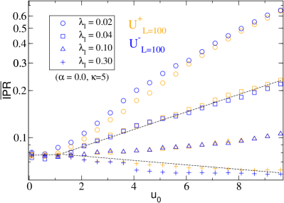
therefore we fix $\kappa$ as well as consider uncorrelated disorder $\alpha=0$ where Anderson localization of all states is a proven fact in one dimension for vanishing interaction. To obtain a measure that characterizes the localization property of the whole system (parameters $\kappa,\alpha$ fixed), i.e. for all $\left|E\right\rangle$ satisfying $H_{mp}\left|E\right\rangle=E\left|E\right\rangle$ (cf. Fig. 3) we convolute $\text{IPR}(E)$ extracted from $p_{i}(E)$ with $\text{DOS}(E)$ as performed several times during our numerical studies in Sect. II.2 (cf. Eq. (11)):

$$\overline{\text{IPR}}(\pm u_{0},\lambda_{I})\equiv\int dE~{}\text{IPR}(E)\text{DOS}(E)\quad.$$ (26)

The corresponding result is shown in Fig. 7. As independently predicted by Shepelyansky and Imry localization seems to be invariant under the transformation $U_{ij}\to-U_{ij}$. Moreover, the range $\lambda_{I}$ determines whether the increasing onsite interaction strength $u_{0}$ (weakly) delocalizes or tends to localize the two bosons. This effect sets in when $\left|U_{0}\right|\sim J$, i.e. when the interaction energy becomes comparable to the kinetic contributions in $H_{mp}$.

A plausible argument for the observation that our results yield independence from the sign of the mutual particle interaction relies on a discrete (spatial) symmetry of the Hubbard Hamiltonian Sakmann et al. (2010); Schneider et al. (2010) which we apply to Eq. (19). Suppose we transform the spatial wave function $\langle j|E\rangle$ such that all, say, odd site $j$ contributions are inverted and all even ones are left unchanged. The corresponding operator in the basis $\{\left|j\right\rangle\}$ reads

$$\mathcal{U}\equiv\mathrm{diag}(\dots,-,+,-,+,-,+,\dots)=\mathcal{U}^{+}$$ (27)

and satisfies $1=\mathcal{U}^{2}$, i.e. $\mathcal{U}$ is a unitary transformation. In terms of annihilation (creation) operators one obtains $\mathcal{U}c^{(+)}_{j}\mathcal{U}^{+}=(-)^{j}c^{(+)}_{j}=e^{i\pi j}c^{(+)}_{j}$. Now, the key observation is that

$$\mathcal{U}H_{mp}(U_{0})\mathcal{U}^{+}=-H_{mp}(-U_{0})$$ (28)

approximately holds when averaging over disorder realizations (cf. Eq. (26)), since on average for each set $\{\epsilon_{j}\}$ there will be another one $\{-\epsilon_{j}\}$ when $\alpha=0$. More precisely, if we fix the disorder potential $\{\epsilon_{j}\}$ the solution $H_{mp}(-U_{0})\left|E^{\prime}\right\rangle=E^{\prime}\left|E^{\prime}\right\rangle$ is related to the solution of $H_{mp}(U_{0})\left|E\right\rangle=E\left|E\right\rangle$ with $\{-\epsilon_{j}\}$ by the identifications $E^{\prime}=-E$ and $\left|E^{\prime}\right\rangle=\mathcal{U}\left|E\right\rangle$ which obviously leaves physical observables/localization measures invariant.

Concerning the qualitative different localization properties of the interacting bosons with respect to the range $\lambda_{I}$ we would like to provide some phenomenological argument that may also draw a unified picture of delocalization by

Figure 8: (color online) Impact of correlation ($\alpha>0$, $\alpha=0$ as a reference) on the localization property of two interacting bosons. We picked out two representative branches ($\lambda_{I}=0.04$ and $\lambda_{I}=0.3$) from Fig. 7 to demonstrate that, as expected, correlations tends to delocalize the system. Furthermore we note that the qualtitative result is again independent of the sign of the interaction and it seems that a feature from $\alpha=0$ stays untouched: Namely, small interaction ranges $\lambda_{I}$ (weakly) delocalize with increasing interaction strength $u_{0}$ and with larger $\lambda_{I}$ states localize with respect to increasing $u_{0}$. The numerical data were obtained at $\kappa=5$ from $30$ realizations with $L=100$ sites which we averaged over.

Figure 9: (color online) Finite size analysis of the $\overline{\text{IPR}}^{-1}$ for representative model parameter values that specify the correlated disorder by $\alpha$ and the interaction by its strength $u_{0}$ and range $\lambda_{I}$. Due to the observed sign symmetry we restrict to the case of attractive interaction; the color encoding and point shape is kept as in Fig. 7. Instead of plotting the averaged inverse participation ratio $\overline{\text{IPR}}$ itself, it is more appropriate to consider its inverse since it directly relates to the number of occupied sites of the projected probability distribution $p_{i}$ (cf. Eq. (6) and Eq. (21)).

correlation and interaction. Starting from the case of short-range ($\lambda_{I}\ll 1$), attractive interaction the enhancement of localization may result from the effect of lumping: Assuming sufficiently strong interaction compared to the kinetic energy ($U_{0}\gtrsim J$), once the particles are nearby, they will be tightly bound in space and the quantum dynamics should be governed by this localized behavior. Due to the approximative invariance of the problem to the interaction’s sign the situation (surprisingly) stays unchanged even for repulsive interacting bosons. But according to Fig. 7 the effect of long-range interaction ($\lambda_{I}=0.3$) is qualitatively opposite to the short-range case and we numerically checked that the trend to delocalize with increasing interaction stays up to $\lambda_{I}=1$ (not shown here). One may understand this behavior on the basis of the Fock space Hamilton matrix representation $H_{mp,ff^{\prime}}$ (cf. App. A.2, Eq. (39) and Tab. 1). Since disorder $\epsilon_{i}$ and interaction $U_{ij}$ both contribute to the diagonal elements $H_{mp,ff}$ we may effectively relate the resulting multi-particle Hamiltonian matrix to a corresponding one-dimensional, non-interacting system of size $L(L+1)/2$ with modified disorder $\tilde{\epsilon}_{i^{\prime}=1\dots L(L+1)/2}$ and extended dynamics beyond the nearest neighbor hopping. While short-range interaction just contributes to a few diagonal entries of $H_{mp,ff^{\prime}}$, an increasing interaction range $\lambda_{I}$ affects more and more of those matrix elements. Due to the deterministic character of the $U_{ij}$ (smooth, algebraic long-range decay) it will effectively correlate the $\tilde{\epsilon}_{i^{\prime}}$ of the non-interacting analoguous which we know to yield delocalization for increasing long-range correlation.

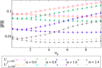
Finally, we want to include long–range correlation ($\alpha>0$) into our toy model of two interacting bosons to directly render the impact of correlation within our localization framework. In Fig. 8 we plot the uncorrelated case from Fig. 7 for two different interaction ranges $\lambda_{I}$ as a reference and, therefore, it becomes clear that correlation among the onsite disorder yields delocalization — as we would expect from our previous experience so far (cf. Sect. II.2 as well as our phenomenological line of reasoning from the preceeding paragraph). However, the feature that short–range ($\lambda_{I}=0.04$) interaction localizes and long-range ($\lambda_{I}=0.3$) interaction seems to delocalize the two bosons for increasing (rescaled) interaction strength $u_{0}$ is similar to the uncorrelated case.

Again, the result seems to be independent of the sign of interaction. Since we have introduced correlation among the $\epsilon_{i}$ our argument according to Eq. (28) should not be valid in general. Therefore we suppose the specific disorder model to intrinsically fulfill the necessary assumption from above. Referring to the limiting case $\alpha\to\infty$ we recognize that $\epsilon_{i}$ becomes $\cos$-like where $\epsilon_{i}\to-\epsilon_{i}$ just shifts the onsite potential by a phase value $\pi$.

We would like to close our discussion by adding comments on the finite size analysis done as well as comparing our investigations to similar literature, especially Ref. [Dukesz et al., 2009], who consider spinless fermions that interact when nearest neighbors to each other — an analogous to the (short-range) onsite interaction scenario for bosons. Dukesz et al. employ the same disorder potential as us and study, among others, the interplay between long-range correlated disorder and interaction for two particles and refer to it as the dilute limit. Their localization detection measure $\left\langle\text{NPC}\right\rangle$ is essentially the inverse of our $\overline{\text{IPR}}$, but with the decisive distinction of being applied directly in Fock space — without any projection back to the lattice we advertised in Sect. III.1. Therefore we will be restricted to a comparison of qualitative features.

Concerning the left upper panel of Fig. 6 in Dukesz et al. we notice (apart from minor deviation for small interaction strength denoted by $\Delta$) the trend of enhanced localization (decreasing $\left\langle\text{NPC}\right\rangle$) for increasing interaction strength. A feature that is confirmed by Fig. 7 for sufficiently small interaction range $\lambda_{I}$ (increasing $\overline{\text{IPR}}$). Aside the non-interacting case ($u_{0}\leftrightarrow\Delta=0$) this qualtitative trend remains when long-range correlation is involved: According to fixed $\alpha$ the different $\left\langle\text{NPC}\right\rangle$–curves in the lower left panel of Fig. 6 decrease in magnitude. Moreover, each single curve supports enhanced delocalization for increasing correlation parameter $0\lesssim\alpha\lesssim 4$.

To study effects of finite size it is actually wise to investigate $\overline{\text{IPR}}^{-1}$, since our discussion on Eq. (6) suggests that it provides some notion on the effective number of occupied sites. It is perhaps that stage where one benefits from the proposed projection prescription of Sect. III.1 again. While $\left\langle\text{NPC}\right\rangle$ measures occupation of the eigenstates $\left|E\right\rangle$ in Fock space our $\overline{\text{IPR}}^{-1}$ directly accounts for the projected probability distribution $p_{i}$ (cf. Eq. (21)) on the one-dimensional lattice with $L$ sites. However, in order to establish a finite size analysis we depicted representative interaction and correlation parameter values $(\alpha,\kappa,u_{0},\lambda_{I})$ and studied the $\overline{\text{IPR}}$ with increasing system size $L$ in Fig. 9. For uncorrelated ($\alpha=0.0$) and correlated ($\alpha=2.4$) disorder we chose two different interaction strengths where there is no significant difference in the $\overline{\text{IPR}}$ with respect to Fig. 8: a) $u_{0}=1$ and b) where the interaction range $\lambda_{I}$ significantly splits the $\overline{\text{IPR}}$ ($u_{0}=9$), respectively.

In the case of uncorrelated disorder (left and middle left panel of Fig. 9) the averaged number of occupied sites $\tilde{L}=\overline{\text{IPR}}^{-1}$ increases less than linear with linear increasing system size. Thus the extrapolation to the thermodynamic limit suggests localized states as for the non-interacting system. However, we would like to point out the increasing deviation of $\tilde{L}$ between short-range and long-range interaction for strong interaction strength $u_{0}$ which we would like to phrase as enhanced delocalization by long-range interaction and which we suggest to keep in mind for further investigations of interacting particles in disordered media. If we turn to the strongly correlated regime ($\alpha>2$) we definitely observe a qualitative difference in the finite size analysis of $\tilde{L}$. Now the $\overline{\text{IPR}}^{-1}$ seems to grow linearly in $L$ and thus the relative number of occupied sites $\tilde{L}/L$ stays constant for $L\to\infty$ assuming that the observed trend remains for $L>120$. Hence strong correlation among the disorder potential $\epsilon_{i}$ delocalizes in analogy to the numerical experience from the non-interacting analysis, Sect. II.2. But again, in the case of $u_{0}=9$ the curves $\tilde{L}(L)$ increasingly deviate for the scenario of short– and long-range interaction, which verifies our proposal of enhanced delocalization by long-range interaction and we scetched a potential (phenomenological) reason by means of a (rough) correspondence to a non-interacting disordered system above.

In summary, we hope that our data demonstrated that there is a complex interplay between correlation and interaction which by means of the Hamilton matrix structure may arise from a similar origin, namely the correlation of the diagonal elements. Furthermore, both effects may compensate each other as seen for $\left.\overline{\text{IPR}}\right|_{\alpha=0,\lambda_{I}=0.04}$ and $\left.\overline{\text{IPR}}\right|_{\alpha=1.6,\lambda_{I}=0.3}$ at $u_{0}\approx 7.5$ in Fig. 8. The numerical study of the interacting bosons supports the independence of localization from the sign of interaction within our picture of multi-particle localization, and we hope that the rather academic treatment of two interacting bosons reveals in experiments with cold gases; at least in principle in the limit of sufficiently low densities. Neverthless we want to remind that all ideas are based on rather phenomenological reasoning and numerical simulations where we are able to point out qualitative trends only. Therefore our results can just pave the way for a more profound understanding on theoretical grounds.

IV Conclusion & Perspectives

To conclude our investigations we briefly summarize what was achieved within our study of the one-dimensional Anderson model. In the first place we analyzed two mechanisms that yield delocalization, namely a correlated disorder potential and mutual interaction between two bosons. By reviewing a known model of correlated disorder from the perspective of exact numerical diagonalization and different (well-established) localization measures, we showed that the process of delocalization is much more complex than observed up to now: Namely, there are reasonable arguments to consider $\alpha=1$ as important for the process of delocalization by correlation. Nevertheless the general trend that increasing correlation yields delocalization was confirmed and localized states approximately vanish for $\alpha\gtrsim 2$. In addition we were able to numerically establish the full parameter dependence of the model system by means of the nearest neighbor distribution (NND) and therefore we went beyond the analysis that focuses on states in the band center. The results suggest that the system eventually becomes delocalized for sufficient large correlation, independent from the disorder strength $\kappa$ which is in accordance with Bloch’s theorem. Nevertheless, we extensively discussed the usage of the NND and tried to convince that it is far less obvious to utilize it as an localization detection measure.

Therefore we introduced a general idea to define localization for multi-particle states of bosons by means of the phenomenology of experiments with cold quantum gases. The examination of two long-range interacting bosons

Figure 10: Illustration of autocorrelation (cf. Eq. (31)) among the onsite disorder $\epsilon_{i}$, Eq. (3). We evaluated $5000$ points $(\epsilon_{i},\epsilon_{i+1})$ with $N=10^{5}$ (cf. Eq. (3)). An increasing correlation parameter $\alpha$ deforms the rotationally invariant density of points $(\epsilon_{i},\epsilon_{i+1})$ to a linear dependence between $\epsilon_{i}$ and $\epsilon_{i+1}$ which can be quantitatively detected by the (linear) autocorrelation $C(d)$. Rotational invariance yields $C(1)=0$ and linear dependence between $\epsilon_{i}$ and $\epsilon_{i+1}$ implies $C(1)=\pm 1$. Note, that even in the case $\alpha=0$ our model disorder is not totally homogeneous in $[-0.5,0.5]\times[-0.5,0.5]$.

on a finite, one-dimensional lattice with (perfect) disorder confirmed the conjecture that the localization property does not dependent on the sign of interaction. We showed that this phenomenon leads back to a discrete symmetry arising when averaging over disorder realizations. Finally the complex interplay of correlation and interaction was studied numerically and by means of phenomenological reasoning on the basis of the Hamilton matrix structure we argued how to relate the impact of interaction to delocalization by correlation known from the non-interacting system.

Although our contribution provides some new insights to the phenomenon of localization, unsolved aspects remain. More precisely, a solid theoretical description of the crossover from localization to delocalization when tuning the (nearly) perfect disorder to the Bloch–like situation of a highly correlated potential is desired. Moreover a more profound understanding of the numerically observed effects of interaction on localization is imperative to obtain further insight to delocalization/localization in the presence of many interacting particles.

Appendix A Numerical Details

This appendix is dedicated to computational details of our work. We especially address the correlated disorder used in the main part and an explicit calculation of the Hamiltonian matrix of two interacting bosons for an arbitrary (finite) number of lattice sites.

A.1 Correlated disorder

Here, we provide some properties of the correlated disorder potential $\epsilon_{i}$ and as a general remark we mention that all our numerical results were averaged over a number of disorder realizations. If we exactly follow the prescription Eq. (3) to obtain $L$ values $\epsilon_{i}$ with correlation parameter $\alpha$ the quantity

$$\delta\equiv\max_{i}\epsilon_{i}-\min_{i}\epsilon_{i}\quad,\quad i=1\dots L$$ (29)

will not be constant in general. To ensure the same disorder strength $\kappa$ for all disorder realizations and system sizes, we always normalize a given chain of $\epsilon_{i}$ values by

$$\epsilon_{i}\to\epsilon_{i}-\min_{i}\epsilon_{i}\to\frac{\Delta}{\delta}\epsilon_{i}\to\epsilon_{i}-\frac{\Delta}{2}$$ (30)

to have $\epsilon_{i}\in[-\frac{\Delta}{2},\frac{\Delta}{2}]$. See also Refs. [Kantelhardt et al., 2000,de Moura and Lyra, 2000] for a related discussion.

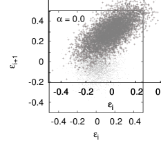
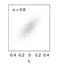
Since we mentioned that $\alpha=0$ refers to nearly perfect disorder, we provide an intuition on that statement in Fig. 10 where we illustrate increasing correlation by plotting $\epsilon_{i}$ versus $\epsilon_{i+1}$ for different (increasing) $\alpha$–values: For $\alpha=0$ the point density is approximately rotationally invariant around $(\epsilon_{i},\epsilon_{i+1})=(0,0)$ and for the autocorrelation function

$$C(d)\equiv\lim_{L\to\infty}\frac{\left\langle\epsilon_{i}\epsilon_{i+d}\right\rangle_{L}-\left\langle\epsilon_{i}\right\rangle_{L}\left\langle\epsilon_{i+d}\right\rangle_{L}}{\sigma_{\epsilon_{i},L}\sigma_{\epsilon_{i+d},L}}\quad,$$ (31)

where

$$\left\langle\epsilon_{i}\right\rangle_{L}\equiv\frac{1}{L}\sum_{i=1}^{L}\epsilon_{i}\quad\text{and}\quad\sigma^{2}_{\epsilon_{i},L}\equiv\left\langle\epsilon^{2}_{i}\right\rangle_{L}-\left\langle\epsilon_{i}\right\rangle^{2}_{L}\quad,$$ (32)

we find $C(1)\approx 0$ for $\alpha=0$. By means of Eq. (31) we can state that the disorder is uncorrelated. But as obvious from Fig. 10 the whole plane $(\epsilon_{i},\epsilon_{i+1})\in[-0.5,0.5]\times[-0.5,0.5]$ ($\Delta=1$) is not uniformly filled with points $(\epsilon_{i},\epsilon_{i+1})$ and therefore an arbitrary onsite potential value $\epsilon_{i}$ can not obviously be followed by any possible $\epsilon_{i+1}$. Thus we refer to the case $\alpha=0$ as weakly correlated. On increasing correlation we observe that the $(\epsilon_{i},\epsilon_{i+1})$ become more and more linearly correlated, i.e. $\epsilon_{i}\approx const.\cdot\epsilon_{i+1}$ and thus $C(1)\approx 1$.

Let us finally sketch one feature of the $\epsilon_{i}$ that arises when approximately computing $C(d)$ to demonstrate the long-range character of the correlated disorder. Let

$$\epsilon(x_{i})=\int_{0}^{\infty}dk~{}k^{-\alpha/2}\cos[kx_{i}+\phi_{k}],\quad x_{i}=i\Delta x$$ (33)

be the continuous version of Eq. (3) and

$$C(d)\propto\lim_{X\to\infty}\frac{1}{X}\int_{0}^{X}dx~{}\epsilon(x)\epsilon(x+d)$$ (34)

that of Eq. (31). Hence we obtain

$$C(d)\propto\frac{1}{2}\int_{0}^{\infty}dk~{}k^{-\alpha}\cos(kd)$$ (35)

which can be analytically solved for $\alpha\in(0,1)$ and we end up with

$$C(d)\propto d^{\alpha-1}\quad 0<\alpha<1\quad.$$ (36)

Hence we have a direct argument at hand why the $\epsilon_{i}$ are long-range correlated: Its spatial autocorrelation decays algebraically (at least in the continuum limit for $\alpha\in(0,1)$) such that increasing $\alpha$ yields a slower decay with distance $d$. Within this picture $\alpha=1$ is also highly correlated and one may argue that delocalization occurs below $\alpha=2$ which is qualitatively supported by our localization measures although the LL agrees pretty well with other results from the literature (cf. discussion in Sect. II.2).

A.2 Matrix representation of two interacting bosons in the modified/interacting Anderson model

For the numerical results on two interacting particles we developed a rather general scheme of the matrix representation in Fock space which allows us to set the numerics for an arbitrary number of sites. Moreover the matrix is banded with a width $\sim L$ which helps to increase the efficiency of the diagonalization routine. As we were inspired by an experimental setup, we used hard–wall/open boundary conditions, i.e. there is no (kinetic) hopping element $J$ (cf. beginning of Sect. (I)) from site $i=1$ to site $L$ and vice versa.

We obtained the matrix structure presented in Tab. 1

$$\footnotesize\left[\begin{array}[]{ccccccccccccccccccccc}x&\times&\lx@intercol\xleftarrow{\hskip 113.81102pt}\hfil\lx@intercol&\lx@intercol\hfil\mathcal{O}(L^{2})\hfil\lx@intercol&\lx@intercol\hfil\xrightarrow{\hskip 113.81102pt}\lx@intercol\\ \times&x&\times&&&&\times&&&&&&&&&&\\ &\times&x&\times&&&\uparrow&\times&&&&&&&&&&&&&\\ &&\times&x&\times&&&&\times&&&&&&&&&&&&\\ &&&\times&x&\times&{\scriptstyle\mathcal{O}(L)}&&&\times&&&&&&&&&&&\\ &&&&\times&x&\downarrow&&&&\times&&&&&&&&&&\\ &\times&&&&&x&\times&&&&&&&&&&&&&\\ &&\times&&&&\times&x&\times&&&\times&&&&&&&&&\\ &&&\times&&&&\times&x&\times&&&\times&&&&&&&&\\ &&&&\times&&&&\times&x&\times&&&\times&&&&&&&\\ &&&&&\times&&&&\times&x&&&&\times&&&&&&\\ &&&&&&&\times&&&&x&\times&&&&&&&&\\ &&&&&&&&\times&&&\times&x&\times&&\times&&&&&\\ &&&&&&&&&\times&&&\times&x&\times&&\times&&&&\\ &&&&&&&&&&\times&&&\times&x&&&\times&&&\\ &&&&&&&&&&&&\times&&&x&\times&&&&\\ &&&&&&&&&&&&&\times&&\times&x&\times&\times&&\\ &&&&&&&&&&&&&&\times&&\times&x&&\times&\\ &&&&&&&&&&&&&&&&\times&&x&\times&\\ &&&&&&&&&&&&&&&&&\times&\times&x&\times\\ &&&&&&&&&&&&&&&&&&&\times&x\\ \end{array}\right]\normalsize$$ (37)

Table 1: Matrix structure of the multi-particle Hamiltonian $H_{mp}$ in the 2-particle basis, Eq. (38) with $L=6$ sites.

where we labeled and ordered the Fock states according to

$$\left|1\right\rangle_{F} = \left|200\dots 0\right\rangle$$

$$\left|2\right\rangle_{F} = \left|110\dots 0\right\rangle$$

$$\left|3\right\rangle_{F} = \left|101\dots 0\right\rangle$$

$$\vdots$$

$$\left|L\right\rangle_{F} = \left|100\dots 1\right\rangle$$

$$\left|L+1\right\rangle_{F} = \left|020\dots 0\right\rangle$$

$$\vdots$$

$$\left|L(L+1)/2\right\rangle_{F} = \left|000\dots 2\right\rangle$$ (38)

with $\left|n_{1}n_{2}\dots n_{L}\right\rangle$ indicating the number $n_{i}$ of bosons at site $i$ and the matrix structure was exemplarily evaluated for $L=6$. Entries $\times$ denote (constant) kinetic off–diagonal values and $x$ refers to the diagonal elements that are determined by the correlated disorder terms $\epsilon_{i}$ and the interaction potential $U_{ij}$. If we write the Hamiltonian matrix elemtens as

$$H_{mp,ff^{\prime}}\equiv\left\langle f\left|H_{mp}\right|f^{\prime}\right\rangle_{F}$$ (39)

the generalization to an arbitrary number of sites $L$ reads:

	$\square$ diagonal element $H_{mp,ff}$ contributions
$f$:	1	2	…	L	L+1	L+2	…	L(L+1)/2-1	L(L+1)/2
$\epsilon_{i}c^{+}_{i}c_{i}$:	$\epsilon_{1}+\epsilon_{1}$	$\epsilon_{1}+\epsilon_{2}$	$\dots$	$\epsilon_{1}+\epsilon_{L}$	$\epsilon_{2}+\epsilon_{2}$	$\epsilon_{2}+\epsilon_{3}$	$\dots$	$\epsilon_{L-1}+\epsilon_{L}$	$\epsilon_{L}+\epsilon_{L}$
$U_{i,j}c_{i}^{+}c_{j}^{+}c_{i}c_{j}$:	$U^{\pm}_{L}(0)$	$U^{\pm}_{L}(1)$	$\dots$	$U^{\pm}_{L}(L-1)$	$U^{\pm}_{L}(0)$	$U^{\pm}_{L}(1)$	$\dots$	$U^{\pm}_{L}(1)$	$U^{\pm}_{L}(0)$
	$\square$ first off–diagonal elements $H_{mp,ff+1}/J$
$Jc^{+}_{i+1}c_{i}$:	$\sqrt{2}$	$1$	$\dots$	$0$	$\sqrt{2}$	$1$	$\dots$	$0$	$-$
	$\square$ remaining off–diagonal elements $H_{mp,ff^{\prime}}$
$Jc^{+}_{i+1}c_{i}$:	all remaining off–diagonal elements have magnitude $J$. In the $j$th off–diagonal ($j\geq 1$) there are $j$
	non-zero elements: $H_{mp,ff+j}$ with
	$f=L-\sum^{j}_{r=1}r=L-j(j+1)/2~{},\quad\dots~{},\quad L-j(j+1)/2-(j-1)\quad.$

References

- Anderson (1958) P. W. Anderson, Phys. Rev. 109, 1492 (1958).
- Altland and Simons (2010) A. Altland and B. Simons, “Condensed matter field theory,” (Cambridge University Press, 2010) Chap. 2.2, 2nd ed.
- Abrahams et al. (1979) E. Abrahams, P. W. Anderson, D. C. Licciardello, and T. V. Ramakrishnan, Phys. Rev. Lett. 42, 673 (1979).
- Haake (2004) F. Haake, Quantum Signatures of Chaos (Springer–Verlag, 2004).
- Fürstenberg (1963) H. Fürstenberg, Trans. Am. Math. Soc. 108, 377 (1963).
- Bloch (1928) F. Bloch, Z. Phys. 52, 555 (1928).
- García-García and Cuevas (2009) A. M. García-García and E. Cuevas, Phys. Rev. B 79, 073104 (2009).
- de Moura and Lyra (1998) F. A. B. F. de Moura and M. L. Lyra, Phys. Rev. Lett. 81, 3735 (1998).
- Schubert et al. (2005) G. Schubert, A. Weiße, and H. Fehske, Phys. B 359–361, 801 (2005).
- Kaya (2007) T. Kaya, Eur. Phys. J. B 55, 49 (2007).
- Shima et al. (2004) H. Shima, T. Nomura, and T. Nakayama, Phys. Rev. B 70, 075116 (2004).
- Billy et al. (2008) J. Billy, V. Josse, Z. Zuo, A. Bernard, B. Hambrecht, P. Lugan, D. Clément, L. Sanchez-Palencia, P. Bouyer, and A. Aspect, Nature 453, 891 (2008).
- Sanchez-Palencia and Lewenstein (2010) L. Sanchez-Palencia and M. Lewenstein, Nat. Phys. 6, 87 (2010).
- Anderson (1978) P. W. Anderson, Science 201, 307 (1978).
- Fleishman and Anderson (1980) L. Fleishman and P. W. Anderson, Phys. Rev. B 21, 2366 (1980).
- Gurarie et al. (2009) V. Gurarie, L. Pollet, N. V. Prokof’ev, B. V. Svistunov, and M. Troyer, Phys. Rev. B 80, 214519 (2009).
- Griesmaier et al. (2005) A. Griesmaier, J. Werner, S. Hensler, J. Stuhler, and T. Pfau, Phys. Rev. Lett. 94, 160401 (2005).
- Stuhler et al. (2005) J. Stuhler, A. Griesmaier, T. Koch, M. Fattori, T. Pfau, S. Giovanazzi, P. Pedri, and L. Santos, Phys. Rev. Lett. 95, 150406 (2005).
- Osborne and Provenzale (1988) A. R. Osborne and A. Provenzale, Phys. D 35, 357 (1988), sec. 3.
- Moore (1973) E. J. Moore, J. Phys. C: Solid State Phys. 6, 1551 (1973).
- Kramer and MacKinnon (1993) B. Kramer and A. MacKinnon, Rep. Prog. Phys. 56, 1469 (1993), chap. 5.2.
- Brody et al. (1981) T. A. Brody, J. Flores, J. B. French, P. A. Mello, A. Pandey, and S. S. M. Wong, Rev. Mod. Phys. 53, 385 (1981).
- Gómez et al. (2002) J. M. G. Gómez, R. A. Molina, A. Relaño, and J. Retamosa, Phys. Rev. E 66, 036209 (2002).
- Efetov (2004) K. B. Efetov, in Applications of Random Matrices in Physics (Springer, 2004) pp. 104–138.
- Simons and Altshuler (1996) B. D. Simons and B. L. Altshuler, in Mesoscopic Quantum Physics: Proceedings of the LXI. Les Houches Summer School (Elsevier, 1996).
- Feingold et al. (1985) M. Feingold, S. Fishman, D. R. Grempel, and R. E. Prange, Phys. Rev. B 31, 6852 (1985).
- Shklovskii et al. (1993) B. I. Shklovskii, B. Shapiro, B. R. Sears, P. Lambrianides, and H. B. Shore, Phys. Rev. B 47, 11487 (1993).
- Jacquod (1998) P. Jacquod, Phys. Rev. Lett. 81, 1913 (1998).
- Cuevas (1999) E. Cuevas, Phys. Rev. Lett. 83, 140 (1999).
- Dyson (1962) F. J. Dyson, J. Math. Phys. 3, 140 (1962).
- Li et al. (2005) W. Li, P. J. Tanner, and T. F. Gallagher, Phys. Rev. Lett. 94, 173001 (2005).
- Singer et al. (2004) K. Singer, M. Reetz-Lamour, T. Amthor, L. G. Marcassa, and M. Weidemüller, Phys. Rev. Lett. 93, 163001 (2004).
- Aizenman and Warzel (2009) M. Aizenman and S. Warzel, Comm. Math. Phys. 290, 903 (2009).
- Basko et al. (2006) D. M. Basko, I. L. Aleiner, and B. L. Altshuler, Ann. Phys. 321, 1126 (2006).
- Berkovits and Avishai (1998) R. Berkovits and Y. Avishai, Phys. Rev. Lett. 80, 568 (1998).
- Shepelyansky (1994) D. L. Shepelyansky, Phys. Rev. Lett. 73, 2607 (1994).
- Imry (1995) Y. Imry, Europhys. Lett. 30, 405 (1995).
- Frahm et al. (1995) K. Frahm, A. Müller-Groeling, J.-L. Pichard, and D. Weinmann, Europhys. Lett. 31, 169 (1995).
- Römer and Schreiber (1997) R. A. Römer and M. Schreiber, Phys. Rev. Lett. 78, 515 (1997).
- Sakmann et al. (2010) K. Sakmann, A. I. Streltsov, O. E. Alon, and L. S. Cederbaum, Phys. Rev. A 82, 013620 (2010).
- Schneider et al. (2010) U. Schneider, J. P. R. L. Hackermüller, S. Will, S. Braun, T. Best, I. Bloch, E. Demler, S. Mandt, D. Rasch, and A. Rosch, “Breakdown of diffusion: From collisional hydrodynamics to a continuous quantum walk in a homogeneous Hubbard model,” (2010), app. A.3, arXiv:1005.3545v1 .
- Dukesz et al. (2009) F. Dukesz, M. Zilbergerts, and L. F. Santos, New J. Phys. 11, 043026 (2009).
- Kantelhardt et al. (2000) J. W. Kantelhardt, S. Russ, A. Bunde, S. Havlin, and I. Webman, Phys. Rev. Lett. 84, 198 (2000).
- de Moura and Lyra (2000) F. A. B. F. de Moura and M. L. Lyra, Phys. Rev. Lett. 84, 199 (2000).
- Strogatz (1994) S. Strogatz, “Nonlinear dynamics and chaos – With applications in physics, biology, chemistry and engineering,” (Perseus Books Publishing, 1994) Chap. 10.5.
- Ketterle and Zwierlein (2008) W. Ketterle and W. Zwierlein, in Proceedings of the International School of Physics ’Enrico Fermi’ (2008) arXiv:cond-mat/9904034v2 .