An Alternating Direction Algorithm for Matrix Completion with Nonnegative Factors

Abstract. This paper introduces an algorithm for the nonnegative matrix factorization-and-completion problem, which aims to find nonnegative low-rank matrices $X$ and $Y$ so that the product $XY$ approximates a nonnegative data matrix $M$ whose elements are partially known (to a certain accuracy). This problem aggregates two existing problems: (i) nonnegative matrix factorization where all entries of $M$ are given, and (ii) low-rank matrix completion where nonnegativity is not required. By taking the advantages of both nonnegativity and low-rankness, one can generally obtain superior results than those of just using one of the two properties. We propose to solve the non-convex constrained least-squares problem using an algorithm based on the classic alternating direction augmented Lagrangian method. Preliminary convergence properties of the algorithm and numerical simulation results are presented. Compared to a recent algorithm for nonnegative matrix factorization, the proposed algorithm produces factorizations of similar quality using only about half of the matrix entries. On tasks of recovering incomplete grayscale and hyperspectral images, the proposed algorithm yields overall better qualities than those produced by two recent matrix-completion algorithms that do not exploit nonnegativity.

Keywords. nonnegative matrix factorization, matrix completion, alternating direction methd, hyperspectral unmixing

MSC. 15A83, 65F30, 90C26, 90C90, 94A08

1 Introduction

This paper introduces an algorithm for the following problem:

Definition 1 (Nonnegative matrix factorization / completion (NMFC)).

Given samples $M_{i,j}$, $(i,j)\in\Omega\subset\{1,\ldots,m\}\times\{1,\ldots,n\}$, of a nonnegative rank-$r$ matrix $M\in\mathbb{R}^{m\times n}$, find nonnegative matrices $X\in\mathbb{R}^{m\times q}$ and $Y\in\mathbb{R}^{q\times n}$ such that $\|M-XY\|_{F}$ is minimized.

Note that $q$ is not necessarily set to equal $r$. Firstly, not all rank-$r$ nonnegative matrices have nonnegative factors of size $r$. For some of them, the available size of nonnegative factors is strictly greater than $r$. Secondly, when $M$ is approximately low-rank, i.e. the singular values of $M$ have a fast-decaying distribution, one often sets $q$ to be the estimated rank or the number of significant singular values. This resulting problem can be called approximate NMFC. In general, depending on data and applications, $q$ can be either equal, less than, or greater than $r$.

NMFC is a combination of nonnegative matrix factorization (NMF) — which finds nonnegative factors of a nonnegative matrix given all of its entries — and low-rank matrix completion (LRMC) — which recovers $M$ from an incomplete set of its entries without assuming nonnegativity. Mathematically, given a matrix $M\in\mathbb{R}^{m\times n}$ and $q>0$, we present the three problems with the following models

NMFC: $$\min_{X,Y}\left\{\|\mathcal{P}_{\Omega}(XY-M)\|_{F}^{2}:\begin{array}[]{l}X\in\mathbb{R}^{m\times q},Y\in\mathbb{R}^{q\times n},\\ X_{ij}\geq 0,Y_{ij}\geq 0,\forall~{}i,j\end{array}\right\},$$ (3)

NMF: $$\min_{X,Y}\left\{\|XY-M\|_{F}^{2}:\begin{array}[]{l}X\in\mathbb{R}^{m\times q},Y\in\mathbb{R}^{q\times n},\\ X_{ij}\geq 0,Y_{ij}\geq 0,\forall~{}i,j\end{array}\right\},$$ (6)

LRMC: $$\min_{Z}\left\{\mathrm{rank}(Z):\begin{array}[]{l}Z\in\mathbb{R}^{m\times n},\\ \mathcal{P}_{\Omega}(Z-M)=0\end{array}\right\},$$ (9)

where $\Omega$ indexes the known entries of $M$ and $\mathcal{P}_{\Omega}(A)$ returns a copy of $A$ that zeros out the entries not in $\Omega$. Note that each of the three problems has other models. Examples include weighted least-squares for NMF and NMFC and nuclear-norm minimization for LRMC. While (3) and (6) return $XY$ up to a fixed rank $q$, (9) seeks for a least-rank recovery $Z$. It is well known that models (3)–(9) are non-convex and generally difficult to solve. A recent advance for (9) is that if $M$ is low-rank and the samples $\Omega$ satisfy the so-called incoherence property and are sufficiently large, then a convex problem based on nuclear norm minimization can exactly recover $M$ (see the pioneering work [10], as well as recent results [26, 6, 5, 7]).

We are interested in NMFC since it complements NMF and LRMC. NMF has been widely used in data mining such as text mining, dimension reduction and clustering, as well as spectral data analysis. It started to appear in [24, 22, 23] and has become popular since the publication of [18] in 1999. More information on NMF can be found in the survey paper [1], as well as books [8, 9]. Unlike NMF, NMFC assumes that the underlying matrix is incompletely sampled; hence, it leads to saving of sampling time and storage (for data such as images) and has broader applicability. On the other hand, LRMC has recently found a large number of applications including collaborative filtering, which is used by Netflix to infer individual preference from an incomplete set of user preferences [13], global positioning, which discovers the positions of nodes in a network from incomplete pair-wise distances [3], system identification and order reduction, which recovers or reduces the dimension of the state vectors of a linear time-invariant state-space model [20], as well as the background subtraction and structure-from-motion problems in computer vision. A rank-$q$ matrix $M$ can be written as $M=XY$ for matrices $X$ with $q$ columns and $Y$ with $q$ rows. When $X$ and $Y$ are known to be nonnegative a priori, empirical evidence given in Section 3 shows that imposing nonnegativity on the factors improves the recovery quality. In particular, in certain applications such as hyperspectral unmixing, the factors are nonnegative due to their physical nature, so these applications will benefit from NMFC. To summarize, NMFC combines NMF and LRMC, and NMFC is useful when the underlying matrix has both low rank and nonnegative factors.

1.1 Related Algorithms

There are two algorithms that have been widely used for NMF: the alternating least squares (ALS) in [24] and multiplicative updating (Mult) in [19]. The former algorithm alternatively updates factor matrices $X$ and $Y$ to reduce the least-squares cost $\|XY-M\|_{F}^{2}$. The closed-form updates are given as

$$X_{{\mathrm{new}}} \leftarrow \max\{0,MY^{\top}(YY^{\top})^{\dagger}\},$$

$$Y_{\mathrm{new}} \leftarrow \max\{0,(X^{\top}X)^{\dagger}X^{\top}M\},$$

where $\max\{\cdot,\cdot\}$ is applied component-wise and ${\dagger}$ denotes pseudo-inverse. The algorithm Mult has much cheaper multiplicative updates

$$(X_{\mathrm{new}})_{ij} \leftarrow X_{ij}(MY^{\top})_{ij}/(XYY^{\top}+\epsilon)_{ij},~{}\forall~{}i,j,$$

$$(Y_{\mathrm{new}})_{ij} \leftarrow Y_{ij}(X^{\top}M)_{ij}/(X^{\top}XY+\epsilon)_{ij},~{}\forall~{}i,j,$$

which do not involve matrix inversion. Starting from a nonnegative initial matrix $Y$, $X$ and $Y$ remain nonnegative during the iterations of Mult. The algorithm presented in this paper also applies to NMF if a complete sample set $\Omega$ is used. The resulting algorithm, which has been studied in paper [34], is simpler and compares favorably with ALS and Mult in terms of both speed and solution quality. In fact, the proposed algorithm in this paper extends the work in [34], and both algorithms are based on the algorithm of alternating direction method of multipliers (ADM) [12, 11, 2, 28, 32, 30]. Likewise, we can extend the algorithms ALS and Mult to solving NMFC. Extending ALS is as straightforward as adopting the least-square cost $\|\mathcal{P}_{\Omega}(XY-M)\|_{F}^{2}$ and deriving the corresponding updates. One simple approach to extend Mult is to replace $M$ by $\tilde{M}\in\mathbb{R}^{m\times n}$, defined component-wise by $\tilde{M}_{ij}=M_{ij}\mathbf{1}_{(i,j)\in\Omega}$, i.e. $\tilde{M}$ is a copy of $M$ with the unsampled entries set to 0. Drawing conclusions based on the comparative results in [34], we believe that ADM based methods deliver higher-quality solutions in shorter times.

There are also several algorithms for LRMC. Since LRMC can complete a matrix and return factors that happen to be (approximately) nonnegative, we shall briefly review a few well-known LRMC algorithms and compare them to the proposed algorithm. Singular value thresholding (SVT) [4] and fixed-point shrinkage (FPCA) [21] are two well-known algorithms. SVT applies the linearized Bremgan iterations [33] to the unconstrained nuclear-norm model of LRMC:

$$\min\lambda\|Z\|_{*}+(1/2)\|\mathcal{P}_{\Omega}(Z-M)\|_{F}^{2}.$$ (10)

FPCA solves the same model using iterations based on an iterative shrinkage-thresholding algorithm [16]. Furthermore, classic alternating direction augmented Lagrangian methods have been applied to solving (10) or its variant with constraints $\mathcal{P}_{\Omega}(Z-M)=0$ in [14, 31]. The algorithm LMaFit [29] uses a different model:

$$\min_{X,Y,Z}\{\|XY-Z\|_{F}:\mathcal{P}_{\Omega}(Z-M)=0\}.$$ (11)

The model is solved by a nonlinear successive over-relaxation algorithm [15]. In section 3, we compare the proposed algorithm to FPCA and LMaFit and demonstrate the benefits of taking advantages of factor nonnegativity.

1.2 Organization

The rest of this paper is organized as follows. Section 2 reviews the ADM algorithm and presents an ADM-based algorithm for NMFC. A preliminary convergence result of this algorithm is given in Section 2.3. Section 3 presents the results of numerical simulations, which perform tasks such as decomposing nonnegative matrices, compressing grayscale images, as well as recovering three-dimensional hyperspectral cubes from incomplete samples. Finally, Section 4 concludes this paper.

2 Algorithm and Convergence

2.1 Background: the ADM approach

In a finite-dimensional setting, the classic alternating direction method (ADM) solves structured convex programs in the form of

$$\underset{x\in\mathcal{X},y\in\mathcal{Y}}{\min}f(x)+g(y),\text{s.t.}~{}Ax+By=c,$$ (12)

where $f$ and $g$ are convex functions defined on closed subsets $\mathcal{X}$ and $\mathcal{Y}$ of a finite-dimensional space, respectively, and $A,B$ and $c$ are matrices and vector of appropriate sizes. The augmented Lagrangian of (12) is

$$\mathcal{L}_{A}(x,y,\lambda)=f(x)+g(y)+\lambda^{T}(Ax+By-c)+\frac{\beta}{2}\|Ax+By-c\|_{2}^{2},$$

where $\lambda$ is a Lagrangian multiplier vector and $\beta>0$ is a penalty parameter.

The classic alternating direction method is an extension of the augmented Lagrangian multiplier method [17, 25, 27]. It performs minimization with respect to $x$ and $y$ alternatively, followed by the update of $\lambda$; that is, at iteration $k$,

$$x^{k+1} \leftarrow\underset{x\in\mathcal{X}}{\arg\min}\mathcal{L}_{A}(x,y^{k},\lambda^{k}),$$ (13a)

$$y^{k+1} \leftarrow\underset{y\in\mathcal{Y}}{\arg\min}\mathcal{L}_{A}(x^{k+1},y,\lambda^{k}),$$ (13b)

$$\lambda^{k+1} \leftarrow\lambda^{k}+\gamma\beta(Ax^{k+1}+By^{k+1}-c),$$ (13c)

where $\gamma\in(0,1.618)$ is a step length. While (13a) only involves $f(x)$ in the objective and (13b) only involves $g(y)$, the classic augmented Lagrangian method requires a minimization of $\mathcal{L}_{A}(x,y,\lambda^{k})$ with respect to $x$ and $y$ jointly, i.e., replacing (13a) and (13b) by

$$(x^{k+1},y^{k+1})\leftarrow\underset{x\in\mathcal{X},y\in\mathcal{Y}}{\arg\min}\mathcal{L}_{A}(x,y,\lambda^{k}).$$

As the minimization couples $f(x)$ and $g(y)$, it can be much more difficult than (13a) and (13b).

2.2 Main Algorithm

To facilitate an efficient use of ADM, we consider an equivalent form of (3):

$${\begin{array}[]{ll}\min_{(U,V,X,Y,Z)}&\frac{1}{2}\|XY-Z\|_{F}^{2}\\ \mathrm{s.t.}&X=U,Y=V,\\ &U\geq 0,V\geq 0,\\ &\mathcal{P}_{\Omega}(Z-M)=0,\end{array}}$$ (18)

where $X,U\in\mathbb{R}^{m\times q}$ and $Y,V\in\mathbb{R}^{q\times n}$. The augmented Lagrangian of (18) is

$$\mathcal{L}_{A}(X,Y,Z,U,V,\Lambda,\Pi) = \frac{1}{2}\|XY-Z\|_{F}^{2}+\Lambda\bullet(X-U)$$

$$+\Pi\bullet(Y-V)+\frac{\alpha}{2}\|X-U\|_{F}^{2}+\frac{\beta}{2}\|Y-V\|_{F}^{2},$$

where $\Lambda\in\mathbb{R}^{m\times q}$, $\Pi\in\mathbb{R}^{q\times n}$ are Lagrangian multipliers, $\alpha,\beta>0$ are penalty parameters, and $A\bullet B:=\sum_{i,j}a_{ij}b_{ij}$ for matrices $A$ and $B$ of the same size. We deliberately leave $\mathcal{P}_{\Omega}(Z-M)=0$ in the constraints instead of relaxing them, so only those entries of $Z$ not in $\Omega$ are free variables.

The alternating direction method for (18) is derived by successively minimizing $\mathcal{L}_{A}$ with respect to $X,Y,Z,U,V$, one at a time while fixing others at their most recent values, i.e.,

$$X_{k+1} = \arg\min\mathcal{L}_{A}(X,Y_{k},Z_{k},U_{k},V_{k},\Lambda_{k},\Pi_{k}),$$

$$Y_{k+1} = \arg\min\mathcal{L}_{A}(X_{k+1},Y,Z_{k},U_{k},V_{k},\Lambda_{k},\Pi_{k}),$$

$$Z_{k+1} = \underset{\mathcal{P}_{\Omega}(Z-M)=0}{\arg\min}\mathcal{L}_{A}(X_{k+1},Y_{k+1},Z,U_{k},V_{k},\Lambda_{k},\Pi_{k}),$$

$$U_{k+1} = \underset{U\geq 0}{\arg\min}\mathcal{L}_{A}(X_{k+1},Y_{k+1},Z_{k+1},U,V_{k},\Lambda_{k},\Pi_{k}),$$

$$V_{k+1} = \underset{V\geq 0}{\arg\min}\mathcal{L}_{A}(X_{k+1},Y_{k+1},Z_{k+1},U_{k+1},V,\Lambda_{k},\Pi_{k}),$$

and then updating the multipliers $\Lambda$ and $\Pi$. Specifically, these steps can be written in closed form as

$$X_{k+1} =(Z_{k}Y_{k}^{T}+\alpha U_{k}-\Lambda_{k})(Y_{k}Y_{k}^{T}+\alpha I)^{-1},$$ (19a)

$$Y_{k+1} =(X_{k+1}^{T}X_{k+1}+\beta I)^{-1}(X_{k+1}^{T}Z_{k}+\beta V_{k}-\Pi_{k}),$$ (19b)

$$Z_{k+1} =X_{k+1}Y_{k+1}+\mathcal{P}_{\Omega}(M-X_{k+1}Y_{k+1}),$$ (19c)

$$U_{k+1} =\mathcal{P}_{+}(X_{k+1}+\Lambda_{k}/\alpha),$$ (19d)

$$V_{k+1} =\mathcal{P}_{+}(Y_{k+1}+\Pi_{k}/\beta),$$ (19e)

$$\Lambda_{k+1} =\Lambda_{k}+\gamma\alpha(X_{k+1}-U_{k+1}),$$ (19f)

$$\Pi_{k+1} =\Pi_{k}+\gamma\beta(Y_{k+1}-V_{k+1}),$$ (19g)

where $\gamma\in(0,1.618)$ and $(\mathcal{P}_{+}(A))_{ij}=\max\{a_{ij},0\}$. Since matrix inversions are applied to $q\times q$ matrices, they are relatively inexpensive for $q<\min\{m,n\}$.

2.3 Convergence

Global convergence can be obtained when the classic ADM is applied to two-block convex programs in the form of (12). However, to the best of our knowledge, there is no global convergence result in general for non-convex programs or convex programs with three or more blocks. Note that problem (18) is non-convex and there are three blocks in updates (19). Due to these difficulties, we provide a convergence property of the proposed ADM algorithm that holds only under some assumptions.

A point $(X,Y,Z,U,V)$ satisfies the KKT condition for problem (18) if there exist $\Lambda$ and $\Pi$ such that

$$(XY-Z)Y^{\top}+\Lambda=0,$$ (20a)

$$X^{\top}(XY-Z)+\Pi=0,$$ (20b)

$$\mathcal{P}_{\Omega^{c}}(XY-Z)=0,$$ (20c)

$$\mathcal{P}_{\Omega}(Z-M)=0,$$ (20d)

$$X-U=0,$$ (20e)

$$Y-V=0,$$ (20f)

$$\Lambda\leq 0\leq U,\Lambda\odot U=0,$$ (20g)

$$\Pi\leq 0\leq V,\Pi\odot V=0,$$ (20h)

where $\Omega^{c}$ indexes the unobserved entries of $M$, and $\odot$ denotes component-wise multiplication. To simplify notation, we consolidate all the variables in problem (18) as $W:=(X,Y,Z,U,V),$ and write $\mathcal{L}_{A}(X)$ to represent lagrangian function with respect to $X$ by fixing others at their most recent values.

Theorem 2.1.

Let $\{(W_{k},\Lambda_{k},\Pi_{k})\}$ be a sequence generated by the ADM algorithm (19). If the multiplier sequence $\{(\Lambda_{k},\Pi_{k})\}$ is bounded and satisfies

$$\sum_{k=0}^{\infty}\left(\|\Lambda_{k+1}-\Lambda_{k}\|_{F}^{2}+\|\Pi_{k+1}-\Pi_{k}\|_{F}^{2}\right)<\infty.$$ (21)

Then any accumulation point of $\{W_{k}\}$ satisfies the KKT condition for problem (18). Consequently, any accumulation point of $\{(X_{k},Y_{k})\}$ satisfies the KKT condition for problem (3).

Proof.

First, we claim $W_{k+1}-W_{k}\to 0$, and $(\Lambda_{k+1},\Pi_{k+1})-(\Lambda_{k},\Pi_{k})\to 0$. We begin the proof of this claim by observing that $\mathcal{L}_{A}(W,\Lambda,\Pi)$ is bounded below. This follows from

$$\mathcal{L}_{A}(W,\Lambda,\Pi) = \frac{1}{2}\|XY-Z\|_{F}^{2}+\frac{\alpha}{2}\|X-U+\Lambda/\alpha\|_{F}^{2}-\frac{1}{2\alpha}\|\Lambda\|_{F}^{2}$$

$$+\frac{\beta}{2}\|Y-V+\Pi/\beta\|_{F}^{2}-\frac{1}{2\beta}\|\Pi\|_{F}^{2},$$

and the boundedness of $\{(\Lambda,\Pi)\}$. Furthermore, the lagrangian function $\mathcal{L}_{A}$ is strongly convex with respect to each variable of $X,Y,Z,U$ and $V$. For $X$-variable, it holds for any $X$ and $\Delta X$ that

$$\mathcal{L}_{A}(X+\Delta X)-\mathcal{L}_{A}(X)\geq\partial_{X}\mathcal{L}_{A}(X)^{\top}\Delta X+\alpha\|\Delta X\|_{F}^{2}.$$ (22)

In addition, $X^{*}$ is a minimizer of $\mathcal{L}_{A}(X)$ implies the inequality

$$\partial_{X}\mathcal{L}_{A}(X^{*})^{\top}\Delta X\geq 0.$$ (23)

Combining (22) and (23) and observing $X_{k+1}$ is a minimizer of $\mathcal{L}_{A}(X)$ at the $k$-th iteration, we have

$$\mathcal{L}_{A}(X_{k})-\mathcal{L}_{A}(X_{k+1})\geq\alpha\|X_{k}-X_{k+1}\|_{F}^{2},$$ (24)

and in the same way,

$$\mathcal{L}_{A}(Y_{k})-\mathcal{L}_{A}(Y_{k+1}) \geq\beta\|Y_{k}-Y_{k+1}\|_{F}^{2},$$ (25a)

$$\mathcal{L}_{A}(Z_{k})-\mathcal{L}_{A}(Z_{k+1}) \geq\|Z_{k}-Z_{k+1}\|_{F}^{2},$$ (25b)

$$\mathcal{L}_{A}(U_{k})-\mathcal{L}_{A}(U_{k+1}) \geq\alpha\|U_{k}-U_{k+1}\|_{F}^{2},$$ (25c)

$$\mathcal{L}_{A}(V_{k})-\mathcal{L}_{A}(V_{k+1}) \geq\beta\|V_{k}-V_{k+1}\|_{F}^{2}.$$ (25d)

Let $c:=\min\{\alpha,\beta,1\}$. Then by (24) and (25), we have

$$\mathcal{L}_{A}(W_{k},\Lambda_{k},\Pi_{k})-\mathcal{L}_{A}(W_{k+1},\Lambda_{k+1},\Pi_{k+1})$$

$$= \mathcal{L}_{A}(W_{k},\Lambda_{k},\Pi_{k})-\mathcal{L}_{A}(W_{k+1},\Lambda_{k},\Pi_{k})$$

$$+\mathcal{L}_{A}(W_{k+1},\Lambda_{k},\Pi_{k})-\mathcal{L}_{A}(W_{k+1},\Lambda_{k+1},\Pi_{k+1})$$

$$\geq c\|W_{k}-W_{k+1}\|_{F}^{2}-\frac{1}{\gamma\alpha}\|\Lambda_{k}-\Lambda_{k+1}\|_{F}^{2}-\frac{1}{\gamma\beta}\|\Pi_{k}-\Pi_{k+1}\|_{F}^{2}$$

$$\geq c\|W_{k}-W_{k+1}\|_{F}^{2}-\frac{1}{c\gamma}\left(\|\Lambda_{k}-\Lambda_{k+1}\|_{F}^{2}+\|\Pi_{k}-\Pi_{k+1}\|_{F}^{2}\right).$$

Taking summation of the above inequality and recalling $\mathcal{L}_{A}(W,\Lambda,\Pi)$ is bounded below, we get

$$\sum_{k=0}^{\infty}c\|W_{k}-W_{k+1}\|_{F}^{2}-\sum_{k=0}^{\infty}\frac{1}{c\gamma}\left(\|\Lambda_{k}-\Lambda_{k+1}\|_{F}^{2}+\|\Pi_{k}-\Pi_{k+1}\|_{F}^{2}\right)<\infty.$$

Since the second term on the left of the above inequality is bounded, it follows that

$$\sum_{k=0}^{\infty}c\|W_{k}-W_{k+1}\|_{F}^{2}<\infty,$$

from which we immediately have $W_{k+1}-W_{k}\to 0$. For $(\Lambda_{k+1},\Pi_{k+1})-(\Lambda_{k},\Pi_{k})\to 0$, it directly follows from (21).

Now, we are ready to prove the result of this theorem. First, rearrange the ADM formulas in (19) into

$$(X_{k+1}-X_{k})(Y_{k}Y_{k}^{T}+\alpha I) = -((X_{k}Y_{k}-Z_{k})Y_{k}^{T}$$

$$\quad+\alpha(X_{k}-U_{k})+\Lambda_{k}),$$

$$(X_{k+1}^{T}X_{k+1}+\beta I)(Y_{k+1}-Y_{k}) = -(X_{k+1}^{T}(X_{k+1}Y_{k}-Z_{k})$$

$$\quad+\beta(Y_{k}-V_{k})+\Pi_{k}),$$

$$U_{k+1}-U_{k} = \mathcal{P}_{+}(X_{k+1}+\Lambda_{k}/\alpha)-U_{k},$$ (26c)

$$V_{k+1}-V_{k} = \mathcal{P}_{+}(Y_{k+1}+\Pi_{k}/\beta)-V_{k},$$ (26d)

$$\Lambda_{k+1}-\Lambda_{k} = \gamma\alpha(X_{k+1}-U_{k+1}),$$ (26e)

$$\Pi_{k+1}-\Pi_{k} = \gamma\beta(Y_{k+1}-V_{k+1}),$$ (26f)

and

$$Z_{k+1}=X_{k+1}Y_{k+1}+\mathcal{P}_{\Omega}(M-X_{k+1}Y_{k+1}).$$ (27)

Note $W_{k+1}-W_{k}\to 0$, $\Lambda_{k+1}-\Lambda_{k}\to 0$ and $\Pi_{k+1}-\Pi_{k}\to 0$ imply that the left- and right-hand sides in (26) all go to zero, i.e.,

$$(X_{k}Y_{k}-Z_{k})Y_{k}^{T}+\Lambda_{k} \to 0,$$ (28a)

$$X_{k}^{T}(X_{k}Y_{k}-Z_{k})+\Pi_{k}) \to 0,$$ (28b)

$$\mathcal{P}_{+}(X_{k}+\Lambda_{k}/\alpha)-U_{k} \to 0,$$ (28c)

$$\mathcal{P}_{+}(Y_{k}+\Pi_{k}/\beta)-V_{k} \to 0,$$ (28d)

$$X_{k}-U_{k} \to 0,$$ (28e)

$$Y_{k}-V_{k} \to 0,$$ (28f)

where the terms $\alpha(X_{k}-U_{k})$ and $\beta(Y_{k}-V_{k})$ have been eliminated in (28a) and (28b), respectively, by invoking (28e) and (28f). For any limit point $\hat{W}=(\hat{X},\hat{Y},\hat{Z},\hat{U},\hat{V})$ of sequence $\{W_{k}\}$, there exists subsequence $\{W_{n_{k}}\}$ converging to $\hat{W}$. The boundedness of $\{(\Lambda_{k},\Pi_{k})\}$ implies the existence of a sub-subsequence $\{(\Lambda_{n_{k_{j}}},\Pi_{n_{k_{j}}})\}$ of $\{(\Lambda_{n_{k}},\Pi_{n_{k}})\}$ converging to some point $(\hat{\Lambda},\hat{\Pi})$. Hence, $(\hat{W},\hat{\Lambda},\hat{\Pi})$ is a limit point of sequence $\{(W_{k},\Lambda_{k},\Pi_{k})\}$. Since (27) exactly means

$$\mathcal{P}_{\Omega}(Z_{k}-M)=0,\text{ and }\mathcal{P}_{\Omega}(X_{k}Y_{k}-Z_{k})=0,$$

then clearly, the first six equations in the KKT conditions (20) are satisfied at the limit point $(\hat{W},\hat{\Lambda},\hat{\Pi})$. The nonnegativity of $\hat{U}$ and $\hat{V}$ are guaranteed by the algorithm construction. Therefore, we only need to verify the non-positivity of $\hat{\Lambda}$ and $\hat{\Pi}$, and the complementarity between $\hat{U}$ and $\hat{\Lambda}$, and between $\hat{V}$ and $\hat{\Pi}$. Now we examine the following two equations derived from (28c) and (28d), respectively,

$$\mathcal{P}_{+}(\hat{X}+\hat{\Lambda}/\alpha)=\hat{U},$$ (29a)

$$\mathcal{P}_{+}(\hat{Y}+\hat{\Pi}/\beta)=\hat{V}.$$ (29b)

Note we have $\hat{X}=\hat{U}\geq 0$. If $\hat{U}_{ij}=\hat{X}_{ij}=0$, then (29a) reduces $\mathcal{P}_{+}(\hat{\Lambda}/\alpha)_{ij}=0$, which implies $\hat{\Lambda}_{ij}\leq 0$. On the other hand, if $\hat{U}_{ij}=\hat{X}_{ij}>0$, then (29a) implies $\hat{\Lambda}_{ij}=0$. This proves the non-positivity of $\hat{\Lambda}$ and the complementarity between $\hat{U}$ and $\hat{\Lambda}$. The same argument can be applied to (29b), due to the identical structure, to prove the non-positivity of $\hat{\Pi}$ and the complementarity between $\hat{V}$ and $\hat{\Pi}$.

We have verified the statement concerning the sequence $\{W_{k}\}$ and problem (18). The statement concerning the sequence $\{(X_{k},Y_{k})\}$ and problem (3) follows directly from the equivalence between the two problems. This completes the proof. ∎

From the proof of Theorem 2.1, we can immediately get the following corollary.

Corollary 2.1.

Let $\{(W_{k},\Lambda_{k},\Pi_{k})\}$ be a sequence generated by the ADM algorithm (19). Whenever the sequence converges, the limit satisfies the KKT conditions.

3 Numerical Results

3.1 Implementation and Parameters

A pseudo code for the proposed algorithm is given in Algorithm 1 below.

Algorithm 1 ADM-based algorithm for NMFC

  Input $A=\mathcal{P}_{\Omega}(M)\in\mathbb{R}^{m\times n}$, integer $q>0$, maxiter $>0$, and $tol>0$.

  Set $\alpha,\beta,\gamma>0$. Set $Y$ as a nonnegative random matrix, $Z=A$, and $U,V,\Lambda,\Pi$ as zero matrices of appropriate sizes.

  for $k=1,\ldots,maxiter$ do

     Update $(X_{k},Y_{k},Z_{k},U_{k},V_{k},\Lambda_{k},\Pi_{k})$ by the formulas (19);

     if a stopping criterion is met then

        exit and output $(X_{k},Y_{k})$

     end if

  end for

The most important parameters are $\alpha,\beta$ and $\gamma$. In our implementation, we set $\gamma=1.618$, and $\beta=n\alpha/m$. The setting $\beta=n\alpha/m$ considers the different sizes of $X$ and $Y$ and balances the penalties for constraints $X=U$ and $Y=V$. The naive setting $\alpha=\beta$ also works for our tests but reduces the speed of convergence. By running a range of numerical experiments, we heuristically scale $A$ so that $\|A\|_{F}=2.5\times 10^{5}$ and select $\alpha=2.0\times 10^{-4}\|A\|_{F}\max(m,n)/q$. They have worked well for our tested matrices, and it is worth mentioning that algorithm 1 can work well for different $\alpha,\beta$ in a fairly large interval. The iteration stops once either one of the following conditions is met:

$$\frac{|f_{k+1}-f_{k}|}{\max(1,|f_{k}|)}\leq tol,$$ (30a)

$$f_{k}\leq tol,$$ (30b)

where $f_{k}=\|\mathcal{P}_{\Omega}(X_{k}Y_{k}-A)\|_{F}/\|A\|_{F}$. All tests were performed on a Lenovo T410 laptop with an i7-620m CPU and 3 gigabytes of memory and running 32-bit Windows 7 and MATLAB 2010b.

3.2 Random Nonnegative Matrices Factorization

We compared the algorithm proposed in [34] with the proposed algorithm 1, where the former algorithm takes complete samples of a random matrix $M$ while the latter algorithm takes 75%, 50%, and 25% samples of the same matrix $M$. While other reported tests in this paper used parameters and stopping rules given above, this test set used different but consistent parameters (which are not optimal for algorithm 1) for both algorithms in order to accurately reveal their performance difference and the difference between NMF and NMFC: $\alpha=\beta=10^{4}$ and $tol=10^{-6}$. We generated each rank-$r$ nonnegative matrix $M\in\mathbb{R}^{m\times n}$ in the form of $M=LDR$, where $L\in\mathbb{R}^{m\times r}$ and $R\in\mathbb{R}^{r\times n}$ were generated by calling MATLAB’s command rand and $D$ is an $r\times r$ diagonal matrix with diagonal elements $1,2,\ldots,r$. Such scaling makes $M$ slightly ill-conditioned. We tested different combinations of $n$ and $m$ and obtained roughly consistent results. Figure 1 depicts the recovery qualities and speeds corresponding to $m=n=500$ and varying $q=r=20$ through $50$. The results are the averages of 50 independent trials.

Figure 1: Matrix completion with different sample rates (SRs). Left: relative error in Frobenious norm; Right: cpu time in seconds. The algorithm in [34] was used for SR=100%. Algorithm 1 was used for SR=70%, 50%, 25%. All tests used the same parameters and stopping tolerances, and results are the averages over 50 independent trials

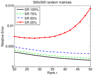
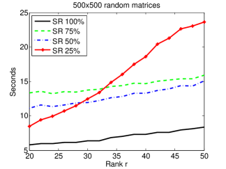
The quality of recovery is similar for SR = 100%, 75%, and 50% for the set of tested matrices. They are all faithful recoveries with relative errors around 0.4%. The relative errors for SR = 75%, and 50% are just slightly worse. The low SR = 25% makes the recovery more difficult. When the ranks $r$ are between 20 and 30, the four error curves are roughly parallel though the red curve (SR = 25%) is worse at relative errors around 0.6%. When $r>30$, 25% of entries seem no longer enough for faithful recovery and consequently, the red curve (SR = 25%) begins to deviate from the others as $r$ increases, and it exhibits a steep upward trend. The difficulty with SR = 25% samples for large $r$ is also shown in terms of cpu seconds. The times for SR = 75% and 50% are about three times as long as those for SR = 100%. Since the times are the averages of merely 50 trials, the curves are not as smooth as they would be if the trials were much more.

The large gap between the red curve in Figure 1(left) and the other curves is largely due to the use of the same stopping tolerance $10^{-6}$. However, SR=25% can reach the similar accuracy of higher SRs if it has a tighter tolerance (e.g., $10^{-7}$) and runs more iterations, at least for $r\leq 30$. In this sense, lower SRs do not necessarily mean much larger errors.

3.3 Overview of Algorithm LMaFit and FPCA

Before more simulation results are presented, let us overview LMaFit and FPCA, which were compared to Algorithm 1 in the next two simulations. LMaFit solves (11) based on a nonlinear successive over-relaxation (SOR) method. From its first-order optimality conditions

$${\begin{array}[]{r}(XY-Z)Y^{\top}=0,\\ X^{\top}(XY-Z)=0,\\ \mathcal{P}_{\Omega^{c}}(Z-XY)=0,\\ \mathcal{P}_{\Omega}(Z-M)=0.\end{array}}$$

the nonlinear SOR scheme is derived as

$${\begin{array}[]{rcl}X_{k+1}&=&Z_{k}Y_{k}^{\top}(Y_{k}Y_{k}^{T})^{\dagger},\\ X_{k+1}(\omega)&=&\omega X_{k+1}+(1-\omega)X_{k},\\ Y_{k+1}&=&(X_{k+1}(\omega)^{\top}X_{k+1}(\omega))^{\dagger}(X_{k+1}(\omega)^{\top}Z_{k}),\\ Y_{k+1}(\omega)&=&\omega Y_{k+1}+(1-\omega)Y_{k},\\ Z_{k+1}(\omega)&=&X_{k+1}(\omega)Y_{k+1}(\omega)+\mathcal{P}_{\Omega}(M-X_{k+1}(\omega)Y_{k+1}(\omega)),\end{array}}$$

where the weight $\omega\geq 1$. One of its stopping criterions is the same as (30a). In our tests described below, we set tol = $10^{-5}$ for Alg 1 and LMaFit and chose different maximum numbers of iterations based on the size of recovered matrix, which will be specified below. We applied the rank-estimation technique coming with LMaFit (hence, we did not fix $q$ for LMaFit).

FPCA solves convex problems in the form of

$$\min\mu\|X\|_{*}+\frac{1}{2}\|\mathcal{A}(X)-b\|_{2}^{2},$$

which includes (10) as a special case by setting the linear operator $\mathcal{A}$ to $\mathcal{P}_{\Omega}$. Introducing $h(X)=\mathcal{A}^{*}(\mathcal{A}(X)-b)$, where $\mathcal{A}^{*}$ is the adjoint of $\mathcal{A}$, we can write the iteration of FPCA as

$$\ \left\{\begin{array}[]{rcl}Y_{k}&\leftarrow&X_{k}-\tau h(X_{k}),\\ X_{k+1}&\leftarrow&S_{\tau\mu}(Y_{k}),\end{array}\right.$$

where $S_{\nu}(\cdot)$ is a matrix singular-value shrinkage operator. In our tests described below, the parameters for FPCA were set to their default values: specifically, tol = $10^{-6}$ and maxiter = $10^{5}$. For the default values of other parameters such as $\tau$ and $\mu$, we refer the reader to [21].

3.4 Hyperspectral Data Recovery

In this subsection, we compare Algorithm 1 with LMaFit [29] and FPCA [21] on recovering three-dimensional hyperspectral images from their incomplete observations. Hyperspectral (or multispectral) imaging is widely used in applications from environmental studies and biomedical imaging to military surveillance. A hyperspectral image is a three-dimensional datacube that records the electromagnetic reflectance of a scene at varying wavelengths, from which different materials in the scene can be identified by exploiting their electromagnetic scattering patterns. We let each hyperspectral datacube be represented by a three-dimensional array whose first two dimensions are spatial and third dimension is wavelength. A hyperspectral datacube can have several hundreds of wavelengths (along the third dimension) but no more than a dozen dominant materials. As a consequence, the spectral vector at every spatial location can be (approximately) linearly expressed by a small set of common vectors, called endmembers or spectral signatures of materials. The number of these basic vectors is much smaller than the number of wavelengths. Since endmembers are naturally nonnegative, a hyperspectral datacube is a set of nonnegative mixtures of a few endmembers, which are also nonnegative. This property makes it possible to recover the endmembers and mixture coefficients from a hyperspectral datacube, and it is called unmixing. Although unmixing is not as simple as NMF, the results of NMF can be used as an initial guess. Compared to NMF, NMFC not only performs initial unmixing but also recovers the datacube from an incomplete set of observed voxels. This advantage will translate to shorter sampling times and perhaps simpler designs of hyperspectral imaging devices.

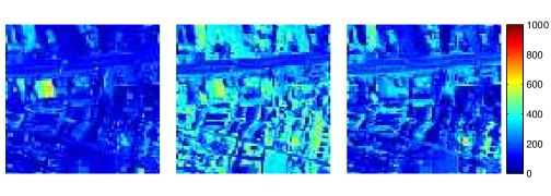
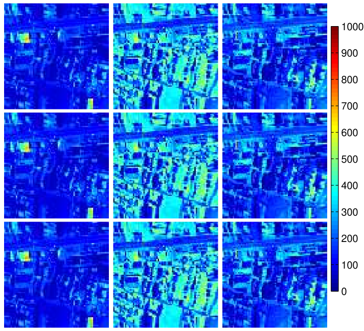
In our simulation, the hyperspectral datacube has 163 wavelengths or slices, and the size of each slice is $80\times 80$. Three selected slices are shown in figure 2. They depict an urban area at three different wavelengths. Roads, roofs, plants, as well as other objects exhibit different intensities. Our simulation begin with reshaping the $80\times 80\times 163$ hyperspectral datacube to a $6400\times 163$ matrix $M$, each slice becoming one column of $M$. While $M$ is full rank, its singular values are fast decaying. We chose the estimate rank $q=30$, and set tol=$10^{-5}$ and maxiter = 2000 for Algorithm 1, and tol=$10^{-5}$ and maxiter = 2000, est_rank=2, rk_inc =3 for LMaFit. The parameters for FPCA were set to their default values.

Figure 2: Original slices of hyperspectral cube

The three algorithms were compared on recovering $M$ from incomplete observations of SR = 30%, 40%, 50%, and their results were compared in terms of peak signal-to-noise ratio (PSNR), as well as mean squared error (MSE). Specifically, given a recovered matrix $\hat{M}$ from incomplete samples of $M\in\mathbb{R}^{m\times n}$, we let

MSE $$:=\frac{1}{mn}\|\hat{M}-M\|_{F}^{2},$$

PSNR $$:=20\log_{10}\left(\frac{\text{MAX}_{\text{I}}}{\sqrt{\text{MSE}}}\right),$$

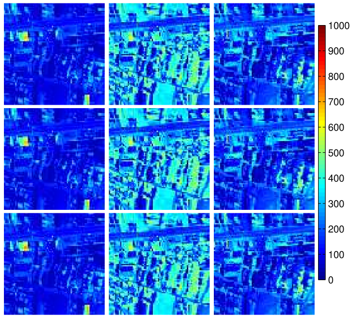
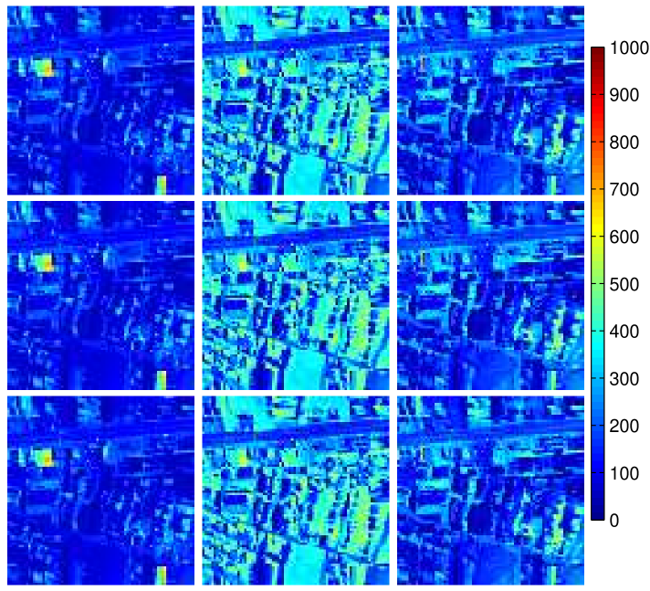
where $\text{MAX}_{\text{I}}$ is the maximum pixel intensity, which is $1023$ in this subsection for the tested hyperspectral data and $1$ in subsection 3.5 for two grayscale images. The results are listed in table 1, and the three slices of the recovered datacube that correspond to those in figure 2 are depicted in figure 3. The results show that Algorithm 1 performs better than FPCA in both CPU time and recovery quality. LMaFit is comparable with algorithm 1 in terms of speed but less accurate. We believe that the use of nonnegativity is a major factor for the superiority of the results of algorithm 1.

Table 1: real data: recovered slices by Algorithm 1, LMaFit, and FPCA. The rank estimate for Algorithm 1 and LMaFit is 30.

problem	Alg 1			LMaFit			FPCA
seed	CPU	PSNR	MSE	CPU	PSNR	MSE	CPU	PSNR	MSE
SR: 30%
3445	27.15	47.71	1.77e+001	14.80	45.05	3.27e+001	39.39	43.31	4.89e+001
31710	26.38	47.52	1.85e+001	31.35	43.08	5.15e+001	39.19	43.56	4.61e+001
43875	27.45	47.50	1.86e+001	40.79	42.26	6.23e+001	38.49	44.35	3.84e+001
69483	25.66	47.71	1.77e+001	42.07	42.20	6.31e+001	39.04	44.20	3.98e+001
95023	25.67	47.48	1.87e+001	32.21	43.02	5.22e+001	39.14	43.13	5.10e+001
SR: 40%
3445	28.46	48.89	1.35e+001	27.51	44.96	3.34e+001	42.85	44.92	3.37e+001
31710	28.66	49.00	1.32e+001	25.99	45.70	2.82e+001	42.96	44.92	3.37e+001
43875	29.81	48.88	1.36e+001	21.89	45.09	3.24e+001	43.32	44.48	3.73e+001
69483	28.24	48.86	1.36e+001	21.38	45.26	3.12e+001	43.99	44.26	3.92e+001
95023	29.10	48.73	1.40e+001	19.31	45.95	2.66e+001	43.87	44.79	3.47e+001
SR: 50%
3445	30.71	49.73	1.11e+001	34.78	44.69	3.55e+001	47.62	44.43	3.77e+001
31710	30.39	49.92	1.07e+001	22.75	46.21	2.50e+001	46.64	43.69	4.47e+001
43875	31.34	49.74	1.11e+001	22.69	46.47	2.36e+001	46.77	44.20	3.98e+001
69483	30.36	49.98	1.05e+001	29.84	45.00	3.31e+001	47.15	44.15	4.02e+001
95023	30.27	49.83	1.09e+001	47.71	44.09	4.08e+001	47.63	44.36	3.84e+001

Figure 3: Recovered slices by Algorithm 1 (first rows), LMaFit (second rows), and FPCA (last rows), respectively; rank estimate for Algorithm 1 and LMaFit is 30

(a) SR = 30%

(b) SR = 40%

(c) SR = 50%

3.5 Tests on images

Despite that natural image recovery from incomplete random samples is not a typical image processing task, we picked it to test algorithm 1, LMaFit, and FPCA since it is easy to visualize their solution qualities. This simulation used two grayscale images, the $768\times 1024$ Kittens and the $1200\times 1600$ Panda, shown in figure 4.

Figure 4: Original images: Kittens (left) and Panda (right)

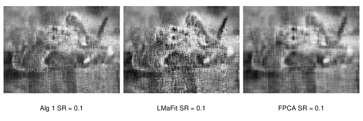
We applied relatively small (thus, challenging) sample rates of SR=10%, 20%, 30% for Kittens and SR=10%, 15%, 20% for Panda. We set tol=$10^{-5}$, and maxiter=2000 for Algorithm 1 and LMaFit and est_rank=2, rk_inc =3 for LMaFit. The parameters for FPCA were set to their default values. The results are given in tables 2 and 3 and the recovered images in figures 5 and 6.

Tables 2 and 3 indicate that FPCA performs slightly better than algorithm 1 in terms of recovery quality but slower when SR is as small as 10% while at this SR, LMaFit performs much worse. With larger SRs such as 20% and 30% for Kittens and SR=15% and 20% for Panda, algorithm 1 is both faster and returns better images than FPCA. With SR=20% and 30%, algorithm 1 is better than LMaFit on Kittens in terms of recovery quality with comparable speed. However, with SR=20%, LMaFit becomes slightly faster than algorithm 1 on Panda with comparable recovery quality. As SR further increases, the three algorithms will return images with almost the same quality while LMaFit is the best in speed.

Table 2: Recover Kittens by Algorithm 1, LMaFit, and FPCA. The rank estimate for Algorithm 1 and LMaFit is 40.

problem	Alg 1			LMaFit			FPCA
seed	CPU	PSNR	MSE	CPU	PSNR	MSE	CPU	PSNR	MSE
SR: 10%
3445	20.98	18.21	1.51e-002	42.96	13.34	4.64e-002	23.01	20.09	9.80e-003
31710	19.00	18.15	1.53e-002	17.34	14.58	3.48e-002	23.30	20.12	9.72e-003
43875	20.03	18.07	1.56e-002	39.95	13.37	4.60e-002	23.40	20.18	9.59e-003
69483	20.33	18.09	1.55e-002	13.60	15.14	3.06e-002	23.04	20.07	9.84e-003
95023	20.06	18.04	1.57e-002	17.89	14.37	3.66e-002	23.25	20.06	9.87e-003
SR: 20%
3445	12.66	23.26	4.72e-003	11.88	21.50	7.08e-003	36.73	22.38	5.78e-003
31710	9.68	23.15	4.84e-003	9.93	21.94	6.39e-003	33.92	22.25	5.95e-003
43875	9.78	23.19	4.80e-003	13.01	21.37	7.30e-003	34.10	22.26	5.94e-003
69483	10.15	23.12	4.87e-003	27.82	19.90	1.02e-002	34.20	22.38	5.78e-003
95023	9.89	23.17	4.82e-003	10.20	21.49	7.10e-003	34.01	22.31	5.87e-003
SR: 30%
3445	9.63	24.53	3.53e-003	9.77	24.11	3.88e-003	54.65	23.44	4.53e-003
31710	7.98	24.48	3.56e-003	8.35	24.10	3.89e-003	54.64	23.30	4.68e-003
43875	9.81	24.48	3.57e-003	12.54	24.03	3.95e-003	55.20	23.47	4.50e-003
69483	7.91	24.45	3.59e-003	5.54	23.78	4.19e-003	54.83	23.40	4.57e-003
95023	8.64	24.46	3.58e-003	9.33	24.06	3.92e-003	54.45	23.33	4.65e-003

Figure 5: Recovered $768\times 1024$ Kittens with estimate rank $q=40$ by Algorithm 1 (left), LMaFit (middle), and FPCA (right)

Table 3: Panda: recovered images by Algorithm 1, LMaFit, and FPCA. The rank estimate for Algorithm 1 and LMaFit is 40.

problem	Alg 1			LMaFit			FPCA
seed	CPU	PSNR	MSE	CPU	PSNR	MSE	CPU	PSNR	MSE
SR: 10%
3445	45.40	23.57	4.40e-003	56.25	18.92	1.28e-002	59.07	23.51	4.46e-003
31710	48.27	23.34	4.64e-003	66.37	18.55	1.40e-002	59.74	23.66	4.30e-003
43875	44.12	23.55	4.42e-003	50.24	19.46	1.13e-002	59.28	23.67	4.29e-003
69483	51.63	23.77	4.20e-003	27.67	20.77	8.37e-003	59.06	23.63	4.34e-003
95023	57.91	23.46	4.51e-003	33.41	19.67	1.08e-002	59.80	23.71	4.26e-003
SR: 15%
3445	32.97	25.83	2.61e-003	40.07	24.79	3.32e-003	73.32	25.26	2.98e-003
31710	29.51	25.74	2.67e-003	37.09	24.79	3.32e-003	72.35	25.15	3.06e-003
43875	32.57	25.84	2.61e-003	15.12	25.20	3.02e-003	72.60	25.14	3.06e-003
69483	29.34	25.80	2.63e-003	31.99	24.84	3.28e-003	72.85	25.13	3.07e-003
95023	26.69	25.80	2.63e-003	17.87	25.20	3.02e-003	71.65	25.03	3.14e-003
SR: 20%
3445	28.45	26.55	2.21e-003	30.25	26.58	2.20e-003	91.00	25.81	2.62e-003
31710	25.79	26.54	2.22e-003	17.71	26.46	2.26e-003	91.23	25.87	2.59e-003
43875	30.69	26.56	2.21e-003	20.51	26.27	2.36e-003	90.20	25.73	2.67e-003
69483	23.13	26.56	2.21e-003	22.06	26.42	2.28e-003	90.40	25.85	2.60e-003
95023	31.05	26.59	2.19e-003	27.80	26.58	2.20e-003	90.67	25.79	2.64e-003

Figure 6: Recovered $1200\times 1600$ Panda for estimate rank $q=40$ by Algorithm 1 (left), LMaFit (middle), and FPCA (right)

4 Conclusions

Among wide applications of nonnegative matrix factorization and those of low-rank matrix completion, there is a rich subset of problems where data matrices can be well approximated by matrix factorizations that are both low-rank and nonnegative, while some of the data (matrix elements) are missing. To best recover missing data, we propose to combine nonnegative matrix factorization and matrix completion, utilizing both nonnegativity and low-rankness in a date recovery formulation. This paper presents our first attempt to solve this non-convex formulation using an algorithm based on the classic alternating direction augmented Lagrangian method. The algorithm has a relatively low per-iteration complexity, especially when the approximation rank is low. Extensive numerical results in this paper indicate that the underlying formulation is useful, and the performance of the alternating direction algorithm is satisfactory. Since global convergence and recovery guarantee results are still largely unknown, we hope that the results of this paper will also motivate further theoretical and numerical studies on this useful problem.

References

- [1] M.W. Berry, M. Browne, A.N. Langville, V.P. Pauca, and R.J. Plemmons. Algorithms and applications for approximate nonnegative matrix factorization. Computational Statistics Data Analysis, 52(1):155–173, 2007.
- [2] Dimitri P. Bertsekas and John N. Tsitsiklis. Parallel and distributed computation: numerical methods. Prentice-Hall, Inc., Upper Saddle River, NJ, USA, 1989.
- [3] P. Biswas, T.C. Lian, T.C. Wang, and Y. Ye. Semidefinite programming based algorithms for sensor network localization. ACM Transactions on Sensor Networks (TOSN), 2(2):188–220, 2006.
- [4] J.F. Cai, E.J. Candès, and Z. Shen. A singular value thresholding algorithm for matrix completion export. SIAM J. Optim., 20:1956–1982, 2010.
- [5] E.J. Candès, X. Li, Y. Ma, and J. Wright. Robust principal component analysis? Journal of the ACM, 58(3), 2011.
- [6] E.J. Candès and B. Recht. Exact matrix completion via convex optimization. Foundations of Computational Mathematics, 9(6):717–772, 2009.
- [7] E.J. Candès and T. Tao. The power of convex relaxation: Near-optimal matrix completion. Information Theory, IEEE Transactions on, 56(5):2053–2080, 2010.
- [8] A. Cichocki, M. Morup, P. Smaragdis, W. Wang, and R. Zdunek. Advances in nonnegative matrix and tensor factorization. Computational intelligence and neuroscience, 2008.
- [9] A. Cichocki, R. Zdunek, A. H. Phan, and S. Amari. Nonnegative Matrix and Tensor Factorizations - Applications to Exploratory Multiway Data Analysis and Blind Source Separation. 2009.
- [10] M. Fazel. Matrix Rank Minimization with Applications. PhD thesis, Stanford University, 2002.
- [11] D. Gabay and B. Mercier. A dual algorithm for the solution of nonlinear variational problems via finite element approximation. Computers and Mathematics with Applications, 2(1):17–40, 1976.
- [12] R. Glowinski and A. Marrocco. Sur lapproximation par elements finis dordre un, et la resolution par penalisation-dualite dune classe de problemes de Dirichlet nonlineaires. Rev. Francaise dAut. Inf. Rech. Oper., pages 41–76, 1975.
- [13] D. Goldberg, D. Nichols, B.M. Oki, and D. Terry. Using collaborative filtering to weave an information tapestry. Communications of the ACM, 35(12):61–70, 1992.
- [14] D. Goldfarb, S. Ma, and Z. Wen. Solving low-rank matrix completion problems efficiently. In proceedings of 47th Annual Allerton Conference on Communication, Control, and Computing, Monticello, Illinois, 2009.
- [15] L Grippo and M Sciandrone. On the convergence of the block nonlinear gauss-seidel method under convex constraints* 1. Operations Research Letters, 26(3):127–136, 2000.
- [16] E. T. Hale, W. Yin, and Y. Zhang. Fixed-point continuation for -minimization: methodology and convergence. SIAM Journal on Optimization, 19(3):1107–1130, 2008.
- [17] M.R. Hestenes. Multiplier and gradient methods. Journal of optimization theory and applications, 4(5):303–320, 1969.
- [18] D.D. Lee and H.S. Seung. Learning the parts of objects by non-negative matrix factorization. Nature, 401(6755):788–791, 1999.
- [19] D.D. Lee and H.S. Seung. Algorithms for Non-Negative Matrix Factorization. Advances in Neural Information Processing Systems, 13:556–562, 2001.
- [20] Z. Liu and L. Vandenberghe. Interior-point method for nuclear norm approximation with application to system identification. SIAM Journal on Matrix Analysis and Applications, 31(3):1235–1256, 2009.
- [21] S. Ma, D. Goldfarb, and L. Chen. Fixed point and Bregman iterative methods for matrix rank minimization. Mathematical Programming, pages 1–33, 2009.
- [22] P. Paatero. Least squares formulation of robust non-negative factor analysis. Chemometrics and Intelligent Laboratory Systems, 37(1):23–35, 1997.
- [23] P. Paatero. The multilinear engine: A table-driven, least squares program for solving multilinear problems, including the n-way parallel factor analysis model. Journal of Computational and Graphical Statistics, 8(4):854–888, 1999.
- [24] P. Paatero and U. Tapper. Positive matrix factorization: A non-negative factor model with optimal utilization of error estimates of data values. Environmetrics, 5(2):111–126, 1994.
- [25] M. J. D. Powell. A method for nonlinear constraints in minimization problems, in optimization. pages 283–298, 1969.
- [26] B. Recht, M. Fazel, and P.A. Parrilo. Guaranteed minimum-rank solutions of linear matrix equations via nuclear norm minimization. SIAM Review, 52(3):471–501, 2010.
- [27] R.T. Rockafellar. The multiplier method of Hestenes and Powell applied to convex programming. Journal of Optimization Theory and Applications, 12(6):555–562, 1973.
- [28] Y. Wang, J. Yang, W. Yin, and Y. Zhang. A new alternating minimization algorithm for total variation image reconstruction. SIAM J. Imaging Sci., 1(3):248–272, 2008.
- [29] Z. Wen, W. Yin, and Y. Zhang. Solving a low-rank factorization model for matrix completion by a non-linear successive over-relaxation algorithm. Rice University CAAM Technical Report TR10-07. Submitted, 2010.
- [30] Zaiwen Wen, Donald Goldfarb, and Wotao Yin. Alternating direction augmented lagrangian methods for semidefinite programming. Mathematical Programming Computation, 2(3-4):203–230, 2010.
- [31] J. Yang and X. Yuan. Linearized augmented lagrangian and alternating direction methods for nuclear norm minimization. To appear in Mathematics of Computation.
- [32] J. Yang, Y. Zhang, and W. Yin. An efficient tvl1 algorithm for deblurring multichannel images corrupted by impulsive noise. SIAM Journal on Scientific Computing, 31:2842–2865, 2008.
- [33] W. Yin, S. Osher, D. Goldfarb, and J. Darbon. Bregman iterative algorithms for -minimization with applications to compressed sensing. SIAM Journal on Imaging Sciences, 1(1):143–168, 2008.
- [34] Y. Zhang. An alternating direction algorithm for nonnegative matrix factorization. Rice Technical Report, 2010.