Random Networks with given rich–club coefficient

Abstract

In complex networks it is common to model a network or generate a surrogate network based on the conservation of the network’s degree distribution. We provide an alternative network model based on the conservation of connection density within a set of nodes. This density is measure by the rich–club coefficient. We present a method to generate surrogates networks with a given rich–club coefficient. We show that by choosing a suitable local linking term, the generated random networks can reproduce the degree distribution and the mixing pattern of real networks. The method is easy to implement and produces good models of real networks.

I Introduction

Many complex networks are single networks in the sense that their structure is unique not one of several. In general, we do not have the equivalent of a physical law to verify if the statistical measures obtained from a single network are expected or exceptional. Instead, a common technique to analyze the properties of a single network is to use statistical randomization methods Manly (1997) to create a reference network which is used for comparison purposes. The procedure consists of using the observed network to generate an ensemble of networks via randomization, usually the reshuffling of the links. The reference network is generated from this ensemble and it is used to assess the significance of a property of the network. To take into consideration the intrinsic structure of the network it is common to use a restricted randomization procedure. The restriction is to reshuffle the connections of the nodes without changing the degree distribution of the nodes $P(k)$ Molloy and Reed (1998), where $P(k)$ is the degree distribution, that is, the fraction of nodes in the network with degree $k$.

Many complex networks contain a small set of nodes that have large numbers of links, the so–called rich nodes. In some networks the rich nodes tend to be tightly interconnected between themselves, forming a rich–club Zhou and Mondragón (2004a). The rich–club is an oligarchy in that it dominates the organization of the whole network. In scale–free networks Albert and Barabási (2002) the connectivity of the rich–club plays an important role in the functionality of the network, for example in the transmission of rumors in social networks Masuda and Konno (2006) or the efficient delivery of information in the Internet Zhou and Mondragón (2004b). The rich–club coefficient measures the density of connection among these group of nodes. This set of nodes can be defined by a ranking scheme Zhou and Mondragón (2004a), by their degree Colizza et al. (2006) or by a network hierarchy McAuley et al. (2007). If the nodes are ranked by non–increasing order of their degree, i.e. the best-connected node is ranked as $r=1$, the second best-connected node is $r=2$ and so on, then the density of connections between the first $r$ nodes is quantified by the rich–club coefficient Zhou and Mondragón (2004a)

$$\Phi(r)=\frac{2E(r)}{r(r-1)},$$ (1)

where $E(r)$ is the number of links between the $r$ nodes and $r(r-1)/2$ is the maximum number of links that these nodes can share. As a function of the node s degree, the rich–club coefficient is Colizza et al. (2006)

$$\phi(k)=\frac{2E_{k}}{N_{k}(N_{k}-1)},$$ (2)

where $N_{k}$ is the number of nodes with degree equal or higher than $k$ and $E_{k}$ is the number of links among these $N_{k}$ nodes. It is known that the rich–club coefficient $\phi(k)$ is a projection of the degree–degree correlation Colizza et al. (2006), is independent of its degree distribution Zhou and Mondragón (2007) and it is non-trivially related to other properties like the clustering coefficient Xu et al. (2010).

It is possible to construct a surrogate network where the degree distribution $P(k)$ is conserved Molloy and Reed (1998); Maslov and Sneppen (2002), the rich–club coefficient $\phi(k)$ is conserved or both of these properties are conserved Zhou and Mondragón (2007). Our aim here, is to build a network model and surrogate random networks based on the rank rich–club coefficient $\Phi(r)$ and show that they are good models of scale–free networks as they tend to reproduce key statistical properties.

Before introducing the model, we would like to remark that the shape of the function $\Phi(r)$ depends on the way that the nodes are ranked. There is an ambiguity when labeling the nodes via a degree–dependent rank. For high degree nodes this is not a problem as the degree tend to be unique so the rank labels these nodes unambiguously. For lower degree nodes, there are many nodes with the same degree. In this case the labeling of the nodes is not unique. It is possible to reduce greatly this redundancy of the labels by using a linear order relationship Nagle (1966), where the degree of the second neighbors is used to disambiguate the labeling. This linear ordering has been used to visualize higher order correlations in the network topology Guo et al. (2007); R.J.Mondragón (2008). We observed that using a degree–only ranking scheme or a linear order ranking has little effect on the statistical properties under consideration here. So in this communication we consider only a degree–dependent ranking scheme.

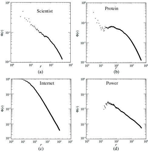
Figure 1 shows $\Phi(r)$ for the Scientists co–authorship (Scientists) Newman (2001), the protein interaction (Protein) Colizza et al. (2005), the AS–Internet (Internet) Mahadevan et al. (2006) and the power grid networks (Power) Watts and Strogatz (1998). We selected these networks as they have been widely used when studying the topological properties of complex network as they have different topological characteristics (e.g. Jamakovic et al. (2009)). These networks have very different connectivities between the high degree nodes. The Internet data has a fully connected core where the top seven nodes are fully connected ($\Phi(7)=1$) in contrast with the power grid network where the top fourteen nodes do not share a link at all ($\Phi(14)=0$).

Figure 1: The rich–club coefficient $\Phi(r)$ for the four networks under study.

II Networks defined by the rich–club coefficient

From equation (1) we have that the number of links that node $r$ shares with the $r-1$ nodes of higher or equal degree is

$$\Delta E(r)=E(r)-E(r-1)=\Phi(r)\frac{r(r-1)}{2}-\Phi(r-1)\frac{(r-1)(r-2)}{2}$$ (3)

where $\Delta E(1)=0$, $\sum_{i=1}^{N}\Delta E(i)=L$ where $L$ is the total number of links and $N$ is the total number of nodes. The term $\Delta E(1)$ is zero, because the node $r=1$ is the top node. The number of links $\Delta E(r)$ is bounded by $0\leq\Delta E(r)\leq r-1$. If $\Delta E(r)$ is known then for $r\geq 2$, $\Phi(r)$ is obtained from the recursive equation

$$\Phi(r)=\frac{2\Delta E(r)+(r-1)(r-2)\Phi(r-1)}{r(r-1)}$$ (4)

with $\Phi(1)=0$.

To determine the network connectivity we need to distribute $\Delta E(r)$ links between node $r$ and the $r^{\prime}\in[1,r-1]$ nodes, for all $r$. Let us assume that $P(r^{\prime},r)$ is the probability that node $r$ connects to node $r^{\prime}<r$, $P(r,r)=0$ as self–loops are not allowed and two nodes can share only one link. Given $\Delta E(r)$ links for $1\leq r\leq N$, we constrain the connectivity of a network by imposing the condition that the average number of links, $\overline{\Delta E}(r)$, between node $r$ and the $r-1$ nodes of lower rank is

$$\overline{\Delta E}(r)=\sum_{i=1}^{r-1}P(i,r)=\Delta E(r).$$ (5)

This last equation defines an ensemble of networks where their average rich–club coefficient $\bar{\Phi}(r)$ is defined by equations (4) and (5). A network from this ensemble satisfies that the average degree $\bar{k}_{r}$ of node $r$ is

$$\bar{k}_{r}=\sum_{r^{\prime}=1}^{N}P(r^{\prime},r)=\Delta E(r)+\sum_{j=r+1}^{N}P(r,j)$$ (6)

with standard deviation $\sigma_{k_{r}}^{2}=\sum_{r^{\prime}=1}^{N}P(r^{\prime},r)(1-P(r^{\prime},r))$. The average number of links is $\bar{L}=\sum_{r}\sum_{r^{\prime}}P(r^{\prime},r)$ with standard deviation $\sigma_{L}^{2}=\sum_{r}\sum_{r^{\prime}}P(r^{\prime},r)(1-P(r^{\prime},r))$ and the average degree of the nearest–neighbors Pastor-Satorras et al. (2001) of a node with degree $k$ is

$$k_{\text{nn}}(k)=\sum_{k^{\prime}=1}^{k_{\rm{max}}}k^{\prime}P(k^{\prime}|k)\approx\frac{1}{N_{k}}\sum_{i=1}^{N}\left(\frac{1}{k}\sum_{j=1}^{N}P(i,j)k_{j}\right)\delta_{k_{i},k}.$$ (7)

In the above equation, the Kronecker delta is introduce to consider only nodes with degree equal to $k$, $N_{k}$ is the number of $k$–degree nodes and the term $1/k$ is a normalization factor.

II.1 Local linking term $T(r^{\prime},r)$

As an ansatz we assume that the probability that there is a link between node $r$ and $r^{\prime}$ can be factorized as

$$P(r^{\prime},r)=T(r^{\prime},r)\,\Delta E(r),\quad r^{\prime}<r,$$ (8)

where $T(r^{\prime},r)$ is a local linking factor. From equation (5) we have that $\sum_{r^{\prime}=1}^{r-1}T(r^{\prime},r)=1$. In here the sample space is the set of all possible combination of links that the node has with the $r-1$ nodes of lower rank, with the restriction that only one link is shared between two nodes. The set of events, used in the definition of the probability, is the different combination that $\Delta E(r)$ links can be shared between node $r$ and the $r-1$ lower rank nodes. Notice that $\Delta E(r)$ is bound by $0\leq\Delta E(r)\leq r-1$.

II.1.1 Egalitarian linking

The simplest case is when the $\Delta E(r)$ links that node $r$ can share with the $r-1$ nodes are evenly distributed, then the probability that node $r$ connects to $r^{\prime}$ is

$$P(r^{\prime},r)=\frac{1}{r-1}\Delta E(r),\quad r^{\prime}<r,$$ (9)

where $T(r^{\prime},r)=1/(r-1)$. For example if node $r$ has a link with all the $r-1$ nodes of lower rank, i.e. $\Delta E(r)=r-1$ then $P(r^{\prime},r)=1$, $r^{\prime}<r$.

II.1.2 Preferential linking

For the case that node $r$ prefers to connect to nodes with lower rank (i.e. higher degree), we propose the preferential linking term $T(r^{\prime},r)=r^{\prime-\alpha}/S(r)$, where $\alpha>0$ is a constant and $S(r)$ is a normalization factor. The probability that there is a link between $r$ and $r^{\prime}$ is

$$P(r^{\prime},r)=\frac{r^{\prime-\alpha}}{S(r)}\Delta E(r)=\left(\frac{r^{\prime-\alpha}}{\sum_{i=1}^{r-1}i^{-\alpha}}\right)\Delta E(r),$$ (10)

where $S(r)=\sum_{i=1}^{r-1}i^{-\alpha}$ to ensure that $\sum_{i=1}^{r-1}P(i,r)=\Delta E(r)$ (see equation 5). Note that it is possible that for some networks the probability function given by equation (10) may be larger than 1, in that case a more suitable $T(r^{\prime},r)$ should be considered.

II.2 Evaluation of the model

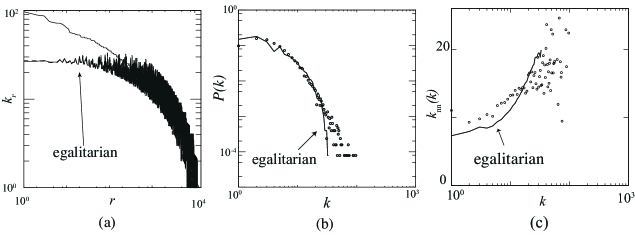
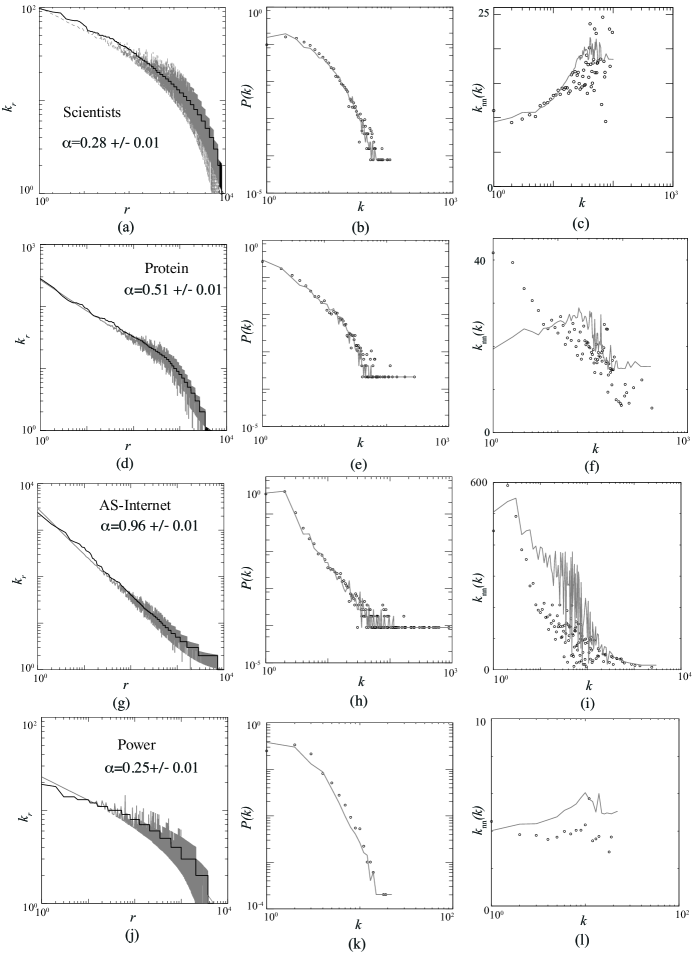
Figure 1(a) shows the rich–club coefficient $\Phi(r)$ as a function of node rank $r$ for the Scientists network. From the data we evaluated $\Phi(r)$ and $\Delta E(r)$. To build a model of the Scientists network we assume that the local linking term is egalitarian and evaluated $P(r,r^{\prime})$, $\bar{k}_{r}$, and $k_{\text{nn}}(k)$ using equations (9), (6) and (7). To obtain an integer value of the node’s degree we used the integer function $|\bar{k}_{r}|$. The degree distribution $P(k)$ was obtained using $|\bar{k}_{r}|$ for all $r$. Figures 2(a) to (c) show that our model resembles the real network, except that the top ranked nodes have similar degrees, which is not true in the real network (see $r<20$ in Figure 2(a)). In fact these nodes have significantly different degrees, which suggests that there is a preferential linking between the high degree nodes. To verify this last statement we created a network model using the preferential linking defined in equation (10). The exponent $\alpha$ was obtained by fitting the average degree of node $\bar{k}_{r}$ using equation (6) against the degree $k_{r}$ from the original network, we did so by obtaining the value of $\alpha$ that minimizes the square of the error $\sum_{r}(k_{r}-\bar{k}_{r})^{2}$ to a precision of $10^{-2}$ in $\alpha$. Figures 3(a)–(c) show that a model based on the preferential linking is a good approximation of the Scientists network.

Figure 2: Topological properties of an egalitarian rich–club network constructed from the Scientists co–authorship network.

We also created a network model based on preferential linking for the Protein interaction network Colizza et al. (2005), the AS–Internet Mahadevan et al. (2006) and the Power grid network Watts and Strogatz (1998). Figures 3(d)–(l) demonstrate that our models closely resemble the degree distribution and give a good approximation to the nearest-neighbors average degree for both assortative (co–authorship) and disassortative (Internet, Protein and Power grid) networks.

Figure 3: The node’s degrees $k_{r}$, their degree distribution $P(k)$ and average degree of the nearest–neighbors $k_{\text{nn}}$ for the four networks under study. The properties of the original network are show in black and their models in gray. For these $\alpha$ values, using linear regression of $(k_{r}-\bar{k}_{r})$ vs. $r$, the regression coefficient $R$ of the networks is between $0.85$ and $0.87$.

III Generating Random Networks With Given Rich-Club Coefficient

For a given network we can generate a surrogate random network which preserves the total number of nodes $N$, links $L$, and the rich–club coefficient $\Phi(r)$ for all $r$. First the $N$ nodes are ranked by their degree and the number of links $\Delta E(r)$ is evaluated from $\Phi(r)$. To create a surrogate network, we create $N$ stub nodes by assigning to each node $r\in[2,N]$, $\Delta E(r)$ links. From $r=2$ to $N$, we connect the $\Delta E(r)$ links between the stub node $r$ and the smaller–ranked $r^{\prime}<r$ nodes. The probability that node $r$ connects to node $r^{\prime}$ is defined by equation (8). We do not allow self–links or that two nodes share more than one link. Notice that $\sum_{r=1}^{N}\Delta E(r)=L$. All of these surrogate networks will have the same rich–club coefficient as the original network because all of them have the same $\Delta E(r)$ for all $r$.

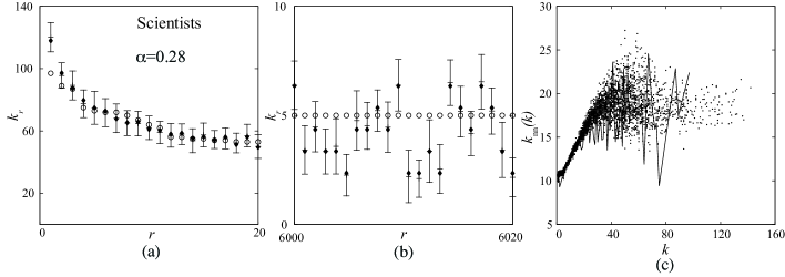
As an example, we illustrate the technique using the Scientists co–authorship collaboration network using preferential linking. Figure 4(a)–(b) show the average node degree as a function of node rank, obtained from 40 surrogate random networks generated using the preferential linking with $\alpha=0.28$. The average degree of the random networks closely (lines with error bars) approximates the degree of the original network (open circles). In the figure we also plotted the average degree obtained from equation (6) (filled diamonds). Notice that we expect a discrepancy between the average degree evaluated from the random networks and the average degree obtained from equation (6). The reason is that the restriction imposed by equation (5) means that the average number of links between node $r$ and the $r^{\prime}<r$ nodes is $\Delta E(r)$. However, the random surrogate networks are generated with the restriction that the number of links between node $r$ and the $r^{\prime}<r$ nodes is exactly $\Delta E(r)$.

Figure 4(c) compares the nearest–neighbors average degree $k_{\text{nn}}(k)$ of the original network (line) against the value obtained by the 40 random networks (scatter dots). It is clear that the random networks resemble well the assortative property of the real network.

Figure 4: (a) Degree $k_{r}$ of the 20 smallest ranked nodes (i.e. $1\leq r\leq 20$), and (b) for $6000\leq r\leq 6020$. The open circle is the original data, the filled diamonds is the average obtained from equation (6) and the line with the error bars obtained from 40 realizations of the random networks. (c) The nearest–neighbors average degree $k_{\text{nn}}(k)$ for the 40 random networks (dots) compared against the value of the original network (solid line).

IV Conclusion

We investigated the properties of random networks defined by a rank–based rich-club coefficient. We show that using a preferential local linking term, we can approximate the degree distribution and the mixing pattern of a variety of real networks. We also introduced a method to generate surrogate random networks conserving the network’s rich–club coefficient. While existing surrogate network models have focused on connectivity of individual nodes, our work provides an alternative method based on the hierarchical structure of a network in terms of link density among a group of nodes.