The Semiclassical Limit of Causal Dynamical
Triangulations
J. Ambjørn, A. Görlich, J. Jurkiewicz, R. Loll, J. Gizbert-Studnicki and T. Trześniewski
a The Niels Bohr Institute, Copenhagen University
Blegdamsvej 17, DK-2100 Copenhagen Ø, Denmark.
email: ambjorn@nbi.dk
b Institute of Physics, Jagellonian University,
Reymonta 4, PL 30-059 Krakow, Poland.
email: atg@th.if.uj.edu.pl, jurkiewicz@th.if.uj.edu.pl,
jakub.gizbert-studnicki@uj.edu.pl, t.trzesniewski@uj.edu.pl
c Institute for Theoretical Physics, Utrecht University,
Leuvenlaan 4, NL-3584 CE Utrecht, The Netherlands.
email: r.loll@uu.nl
d Perimeter Institute for Theoretical Physics,
31 Caroline St. N., Waterloo, Ontario, Canada N2L 2Y5.
Abstract
Previous work has shown that the macroscopic structure of the theory of quantum gravity defined by causal dynamical triangulations (CDT) is compatible with that of a de Sitter universe. After emphasizing the strictly nonperturbative nature of this semiclassical limit we present a detailed study of the three-volume data, which allows us to re-confirm the de Sitter structure, exhibit short-distance discretization effects, and make a first detailed investigation of the presence of higher-order curvature terms in the effective action for the scale factor. Technically, we make use of a novel way of fixing the total four-volume in the simulations.
1 Introduction
Mundane field-theoretical descriptions of quantum gravity have been undergoing a renaissance, thanks to the use of improved renormalization group techniques [1]111building on the original idea of “asymptotic safety” [2], new ideas about the relation between space and time at short scales [3], and a novel way of implementing a lattice regularization of four-dimensional quantum gravity, which takes into account both the dynamical and the causal, Lorentzian nature of spacetime [4].222building on the earlier idea of “dynamical triangulation” as a regularization of quantum gravity [5], but incorporating a concept of micro-causality along the lines of [6] New (and partially overlapping [7, 8, 9, 10, 11]) results obtained in these approaches give rise to the hope that standard tools from quantum field theory – adapted to the situation where spacetime itself is dynamical – are indeed sufficient to construct a theory of quantum gravity nonperturbatively. This is an attractive prospect, since it may imply a large degree of uniqueness, with only a small number of parameters needing to be fine-tuned to get to the correct theory.
In this article we will discuss several aspects of the semiclassical limit of the research program on “Quantum Gravity from Causal Dynamical Triangulations (CDT)”, in which a dynamical lattice provides a geometric UV cut-off. In earlier papers we have reported that the infrared limit of CDT allows an interpretation as the classical solution to Euclidean Einstein gravity with a positive cosmological constant [12, 13, 14, 15, 16] (see also [17] for a pedagogical review). Here we investigate this limit in more detail, including discussions of discretization effects and of the asymmetry between space and time, which appears at the lattice-regularized stage of the CDT set-up.
It is important to bear in mind that what we call the semiclassical limit is a truly nonperturbative limit. This means that the tentative continuum limit of the path integral is to be found in a region of the bare coupling constant space where the entropy of various geometric configurations makes a contribution which is as important as the contribution coming from the exponential of the action. In lower dimensions, this situation is illustrated by the famous Kosterlitz-Thouless transition in the XY model. The XY model is a lattice spin model, whose “spins” are two-dimensional vectors of unit length. In two spatial dimensions, this model has vortex configurations, with an energy per vortex of approximately
| (1) |
where is a coupling constant, a measure of the linear size of the system and the lattice spacing. Ignoring boundary effects, the centre of the vortex can be placed at any one of the lattice points. Saturating the path integral (the partition function) by single-vortex configurations, we obtain333Our present discussion is merely qualitative and meant to highlight the competition between entropy and Boltzmann weights; exact treatments of the Kosterlitz-Thouless transition are given in many textbooks, see, e.g. [18].
| (2) |
We note that the factor is entirely entropic, simply arising from counting the possible single-vortex configurations, and is independent of any “bare” coupling constants (the spin coupling and temperature ). Since the corresponding entropy has the same functional form as the vortex energy, we can express the free energy as
| (3) |
The Kosterlitz-Thouless transition between a low-temperature phase (where vortices play no role) and a high-temperature phase (where vortices are important) occurs when , i.e. when the entropy factor is comparable to the Boltzmann weight of the classical energy. At this point we are far from the naïve weak coupling limit of the lattice spin theory, which is just a Gaussian free field. Instead, the continuum field theory associated with the transition is the sine-Gordon field theory at the coupling constant value where it changes from a super-renormalizable theory to a renormalizable one.
The situation in four-dimensional CDT is analogous, in the sense that the nontrivial structure of the phase diagram reported in [19] results from a competition between the entropy of configurations and the action, precisely as in (3). The analogy goes even further: when written as an effective action for the global scale factor (which plays the role of an order parameter for the gravity case), and in the region of phase space we have identified as possessing a meaningful classical limit, the free energy has the same functional form as the classical action, but with the opposite sign (corresponding to in (3)). This makes it important to understand the semiclassical nature of this phase, and its relation to continuum physics. The investigation of this issue is the main purpose of the present article.
The remainder of this article is organized as follows. In Sec. 2 we recall the set-up of causal dynamical triangulations and introduce a new way of (approximately) fixing the total four-volume of spacetime in the simulations. Using this new prescription, we re-analyze three-volume distributions in Sec. 3 and examine the probability distributions for different values of discrete three-volumes. The latter allows us to exhibit and quantify lattice artifacts for small three-volumes, which occur close to the beginning and end of our quantum universe. In Sec. 4 we introduce a refinement of the spatial slicing, associated with connected layers of the different types of simplicial building blocks. This allows us to analyze the corresponding volume distributions separately, and compare their relative scaling behaviour as a function of the bare coupling constants. In Sec. 5 we return to the task of reconstructing the effective action for the three-volume fluctuations from the computer measurements. In a nontrivial extension of earlier work we look for evidence for the presence of corrections to the effective action associated with curvature-squared terms in the continuum. We summarize and discuss our findings in Sec. 6. The appendix contains a extension of the analysis of Sec. 5 to the situation with a refined spatial slicing.
2 Causal Dynamical Triangulations
In this section, we will review briefly some key ingredients of our approach and give an outline of the methods used. The basic motivation behind quantizing gravity via CDT was explained in [20], and the current set-up described earlier in [4, 13, 16], to which we also refer for further technical details.444An up-to-date reference describing CDT and key results obtained in it is [21].
Assuming that a path integral representation of quantum gravity exists, the basic idea is to provide it with an ultraviolet cut-off by using piecewise linear (“triangulated”) geometries in the quantum superposition. Assigning lengths to the one-dimensional edges of such a triangulation fixes its geometry completely, without the need to introduce coordinates [22], thus also avoiding the redundancies of the usual continuum description of curved geometries. For our purposes, we further restrict the piecewise linear manifolds to those which can be obtained by gluing together two specific types of building blocks (“four-simplices”) with prescribed edge lengths. The typical edge length serves as a geometric UV cut-off and is a measure of the fine-grainedness of the geometry.
Unlike its Euclidean counterpart, CDT also employs a proper-time foliation, with respect to which the topology of space is not allowed to change. Admissible geometries are those which can be constructed by first triangulating spatial slices of constant proper time, which for simplicity we assume to have the topology of . Each three-slice is assembled from identical building blocks, namely, equilateral tetrahedra whose spacelike edges all have length (the spatial lattice spacing or UV cut-off). The gluing and the number of tetrahedra in each slice are arbitrary except for the overall topology and the imposition of local manifold constraints.555Note that neither of these constraints on individual path integral histories will necessarily survive in the continuum limit. Previous results from CDT demonstrate that it can and does happen that the system is driven dynamically to a quantum configuration which is no longer of topology and no longer resembles a four-dimensional manifold. This reflects the nontrivial interplay of “energy” and “entropy” already alluded to in the previous section, which the nonperturbative CDT formulation allows us to capture. The next step consists in connecting neighbouring spatial slices by timelike edges of length (the lattice spacing in time direction), in a way consistent with the “filling” of the spacetime sandwiches by (up to rotations) two types of flat, Lorentzian four-simplices, to wit,
-
•
simplices of type (4,1), which have four vertices in common with the spatial slice at (integer proper) time (thus spanning one of the equilateral tetrahedra making up the slice) and one vertex with the slice at time . Time-reversed building blocks which share one vertex with slice and four vertices with slice are “of type (1,4)”.
-
•
simplices of type (3,2), which have three vertices in common with the spatial slice at (integer proper) time (thus spanning one of the equilateral triangles contained in the slice) and two neighbouring vertices with the slice at time , spanning a spacelike edge there. Time-reversed building blocks which share two vertices with slice and three vertices with slice are “of type (2,3)”.
These four-simplices are glued pairwise along their three-dimensional “faces”, forming a layered, four-dimensional simplicial manifold of topology in the manner just described. In such a piecewise linear geometry the curvature is concentrated at the two-dimensional subsimplices (the triangles) and induces nontrivial rotation angles on vectors which are parallel-transported around them.
Two neighbouring spatial slices labeled by integers and are separated by a proper-time distance in the sense that each timelike edge connecting the two hypersurfaces has this length. Instead of using two lattice spacings and , we usually work with a single and the dimensionless ratio . Expressing in terms of squared lengths allows us (i) to start out in Lorentzian signature, where , and thus , and (ii) to perform for each triangulation an analytic continuation of in the lower-half complex -plane to real, negative , resulting in a piecewise linear geometry of Euclidean signature and length assignments to the edges that in Lorentzian signature used to be timelike. This “Wick rotation” relies on the foliation in proper time. It has no obvious correspondence in the metric continuum formulation (see [23] for a discussion). Under this map, the Einstein-Hilbert action of a given Lorentzian piecewise linear geometry, the so-called Regge action [22], changes according to , where is the Regge action for the corresponding piecewise linear Euclidean geometry with the length assignments . A necessary condition to ensure that the Euclidean four-simplices are nondegenerate is , which will be assumed in what follows. Once the rotation to Euclidean signature has been performed, we redefine , for simplicity of notation.
In our construction of the path integral, we start out with the set of causal piecewise linear Lorentzian geometries described above. In order to perform the sum over these histories, we then rotate each of them to Euclidean signature, so that it will contribute with a real weight . More precisely, we have
| (4) | |||||
where , and are the total numbers of vertices (zero-simplices), of four-simplices of both type (4,1) and type (1,4), and of four-simplices of types (3,2) and (2,3) respectively. The Regge action [22] takes the particularly simple form exhibited in the bottom line of eq. (4) because each CDT contains only two geometrically distinct types of building blocks. The parameter in (4) is proportional to the inverse bare gravitational coupling constant, is a linear function of the bare cosmological and the inverse bare gravitational constant, while is an asymmetry parameter, which for given and can be related to . It is normalized such that (the case of equilateral Euclidean four-simplices) corresponds to .
For technical reasons we perform the numerical simulations at fixed four-volume, which in practice is usually realized by fixing to some target volume . The geometry is updated by using local Monte Carlo moves (c.f. [4, 13, 16]), which in general will change the four-volume. In past papers this was taken care of by modifying the action by a linear term according to , with a parameter controlling the range of fluctuations, and measurements collected only when exactly. Fixing in this delta function-like manner has the side effect of generating a zero mode in the correlation matrix of fluctuations in the spatial three-volume in time, an important quantity in investigating the dynamical behaviour of the quantum universe [16]. Projecting out the zero mode, which is necessary for inverting this matrix, leads to an inconvenient mixing of the remaining modes. To get around this in the present paper, we no longer require that exactly in measurements, but instead let it fluctuate according to the modified action , which eliminates the zero mode. The advantage of using a quadratic term is that it can be treated easily alongside other terms in the action.
In a given simulation, the parameter of the model is fixed by requiring that . The data presented below were taken at , but we checked that the results are essentially unaltered for and . Furthermore, we also checked (at ) that using the total number of four-simplices instead of as the target volume does not change the situation either. Ideally one would like to make as small as possible, but this must be balanced against the fact that smaller -values increase the auto-correlation time.
Depending on the values of the bare couplings in (4), the CDT theory will appear in one out of three different phases A, B or C (see Fig. 6 for a depiction of the phase diagram in the --plane, and [19] for a detailed description). In the present paper we will concentrate on phase C where an extended de Sitter universe has been observed [15, 16, 19]. In this phase we can construct an effective semiclassical action for the scale factor of the universe. Changing the bare coupling constants and will affect the effective coupling constants appearing in this action.
3 Volume distributions reloaded
An interesting observable investigated previously is the typical “shape” or “volume profile” of the quantum universe, more precisely, the average distribution
| (5) |
of spatial volume as function of the discrete proper time .666Equivalently, one can work with the number of three-simplices, where for all interior constant-time slices of the triangulation. What we found is that individual configurations in the well-behaved “de Sitter phase” have a characteristic shape, consisting of a (spatially extended) bulk contribution or “blob” and a separate, thin “stalk”, whose spatial volume for all times stays close to the prescribed minimal cut-off size. Fig. 1 shows an example of the volume distribution of a typical, individual path integral configuration, compared to the average distribution .
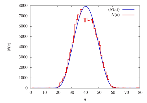
If we compactify the time direction, as is usually done in simulations, the action is symmetric under time translations, permitting us to move the position of the “centre of volume” along the time direction. To determine the average distribution we shift this position for every individual configuration such that its centre coincides with a common reference point on the time axis. For each shifted configuration we measure the three-volume distribution obtained in numerical simulations at some fixed as a function of the shifted time variable , which can be averaged meaningfully over many independent configurations. In [14] it was shown that inside the blob region the average distribution obeys the characteristic scaling relation
| (6) |
where represents proper time and (within numerical accuracy), and and are numerical constants. In the stalk part the average volume is practically constant and independent of . The fact that the numerical data reproduce the distribution (6) with great accuracy remains practically unchanged when the measurements are performed with the new method.
The interpretation of the above results is that the quantum system generates the three-volume distribution of a round four-sphere (i.e. Euclidean de Sitter space) with four-volume , with time steps proportional to the (cosmological) proper time separating the spatial hypersurfaces. The stalk is present only because (i) we have fixed the time period to be larger than the proper-time extension of the universes created, and (ii) we enforce a minimal three-volume of 5 tetrahedra per spatial slice, corresponding to , in keeping with the simplicial manifold character of the spacetime. Although it appears from the simulations that the dynamics of the system wants to drive the three-volume to zero at the two ends of the blob, we prefer to maintain these kinematical restrictions (and thus the stalk region), because they allow us to monitor fluctuations in the time extent of the blob, which would be suppressed if we tried to adjust the time interval to match the blob exactly.
The measurements presented below were taken for the coupling constant values , four-volume and time period , and exhibit a behaviour typical for systems inside the de Sitter phase. The reference time has been fixed to and the distribution symmetrized with respect to . Comparing the volume distributions with relation (6), the range of the blob is roughly in terms of integer times, whereas the stalk region is located in and .
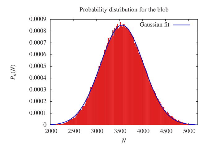
In previous work [14, 15, 16] we have matched the average to the classical solution of a (discretized) mini-superspace action. This semiclassical interpretation is corroborated further by new measurements made of the probability distributions , which for a given time describe the probability that the three-volume is equal to . If the semiclassical picture is indeed correct, these distributions should be approximately Gaussian with a mean equal to and a dispersion . This is exactly what we observe in the range , well inside the blob, as shown in Fig. 2 (top).
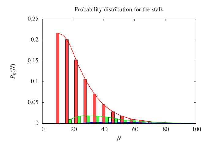
Inside the stalk, the situation is completely different. Not only the average , but also the three-volume distribution is unchanged when we move along the stalk. In addition, we observe short-distance lattice artifacts, in the form of a split of the distribution of three-volumes into three separate families. This is clearly visible in Fig. 2 (bottom), which shows the average three-volume distribution in the stalk for . Inside each family the discrete three-volumes differ by 6, such that we have three sets , and .777Note that by definition is always an even number. Although the presence of the stalk – as we have argued above – is merely a consequence of our kinematical set-up, it cannot simply be ignored, but has to be taken into account in the calculations, for example, when analyzing the covariance matrix of three-volume fluctuations and its inverse. In order to distinguish short-distance artifacts from short-distance physics, it is therefore important to understand the behaviour of the transition region between stalk and blob as best possible.
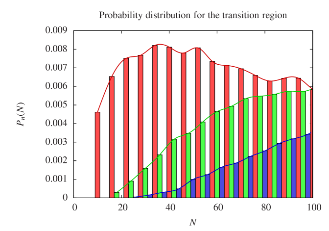
An analogous split into three sets of the three-volume distribution for small volumes is also observed in the region , which smoothly joins the stalk and which we have classified as “inside the blob”, but where is still relatively small. We find that for the distribution again splits into three families. An example for is shown in Fig. 3 (top); the situation is similar for . If in the same transition region one considers higher values of , the split between the three families disappears, but one also notes that the distributions are highly asymmetric and non-Gaussian, as again illustrated for , depicted in Fig. 3 (bottom).
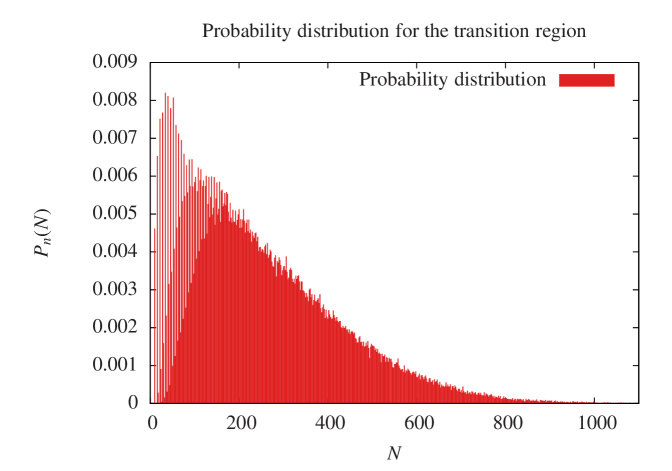
We conclude that lattice artifacts are visible for spatial slices of sizes up to tetrahedra (corresponding to ). This may sound like much, but in reality corresponds to rather small linear distances. This can be understood by comparing the total volume of 100 spatial tetrahedra, , with that of a regular three-sphere, . If we arranged the tetrahedra to approximate such a sphere, we would have , i.e. only a single lattice spacing, with the antipodal distance on the three-sphere being roughly equal to . Viewed like this, it appears rather encouraging that the observed lattice artifacts vanish so quickly as function of the three-volume.
Quantifying the short-distance artifacts for one quantity gives us a good idea of the scale at which they occur for a given four-volume, but still leaves us with the difficulty of disentangling them from genuine quantum-gravity signatures in this and other observables. For example, the non-Gaussian character of the distribution of fluctuations around the sphere (6) at small observed above could indicate new short-distance physics, say, along the lines suggested in the asymptotic safety scenario [24]. We presently do not know how to relate the deviation from the four-sphere at small scale factor described there to our explicit small- “observations”, but it would clearly be interesting to do so.
4 Refining the spatial slicing
An alternative description of the four-dimensional simplicial manifolds contributing to the sum over histories is given in terms of their dual structures, where we assign vertices to the centres of four-simplices and links to the three-dimensional faces between adjacent four-simplices. In the absence of boundaries of the manifold, each dual vertex will have five neighbouring ones, connected by dual links. This dual picture suggests a further subdivision of the original (integer) time steps of the discrete triangulation, as we will now explain.
Integer steps provide natural units for timelike paths in the original lattice if the paths are taken to run only along the timelike888“timelike” refers to the character of the geometric elements before the Wick rotation edges of the four-simplices, which form one-dimensional ‘connectors’ between pairs of adjacent constant-time layers made entirely from spatial tetrahedra. Constructing analogous paths on the dual lattice, at least four steps are required to connect a vertex dual to a (4,1)-simplex at time with a vertex dual to a (4,1)-simplex at the next time step . Labelling the dual vertices by their associated simplex types, such a path is given by a sequence . In addition, we have observed that all dual vertices of types (3,2) and (2,3) between times and and the dual links connecting them form a single closed, connected graph. This makes it natural to assign a time to this layer and study the properties of the distribution of
| (7) |
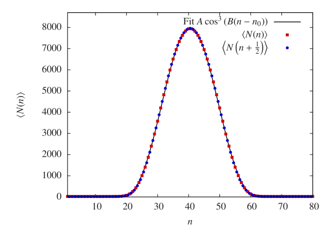
where is the total number of (3,2)- and (2,3)-simplices located between discrete times and . It is not surprising that this distribution is similar to , in fact, by a simple rescaling
| (8) |
(where the constant will depend on the values of the couplings), one can achieve that in the blob range the combined distribution , with now running over both integer and half-integer times, is well approximated by a single, smooth curve according to formula (6). Note that this unification is not global, in the sense that a different rescaling is needed in the stalk part, which is not surprising in view of the different dynamics in this region. Fig. 4 shows the resulting distribution for the standard choice of bare couplings, .
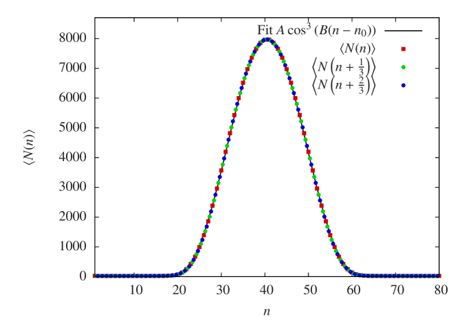
One can push this line of argument further by performing an even finer discrete subdivision of time. As argued above, going forward in time along dual links necessarily takes one through a sequence of different types of four-simplices. Nothing new can be learned by distinguishing between a layer of (4,1)-simplices and that of the adjacent (1,4)-simplices, because they are in one-to-one correspondence (each interior spatial tetrahedron at integer is shared by exactly one (4,1)- and one (1,4)-simplex). By contrast, there is no such relation between the (3,2)- and the (2,3)-simplices. This has motivated us to divide each integer time step into three and study volume distributions separately for the sets of (4,1)-, (3,2)- and (2,3)-simplices contained in each ‘sandwich’ . One finds again that they can be combined into a single, universal distribution by defining
| (9) |
with the same as used before. In (9), and count the number of (3,2)- and (2,3)-simplices, which collectively have been assigned the time labels and , respectively. Fig. 5 illustrates that the sphere fit continues to work beautifully also with respect to this time subdivision. These results underscore that the detailed choices we make at the level of the individual building blocks, in the present example the identification of microscopic time steps, bear little direct relation to the macroscopic aspects of the semiclassical emergent geometry. This may have been anticipated because of the nonperturbative nature of this limit in CDT quantum gravity.
Our next step will be to repeat the above measurement for different values of the bare coupling constants, and to study systematically how the scaling parameter behaves as a function . We are particularly interested in the behaviour inside the de Sitter phase (labelled C in Fig. 6, top) as we approach one of the critical lines, which separate phase C from phases A and B. The set of points in the coupling constant-plane where measurements were taken lies along the T-shape inside phase C.
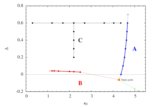
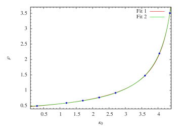
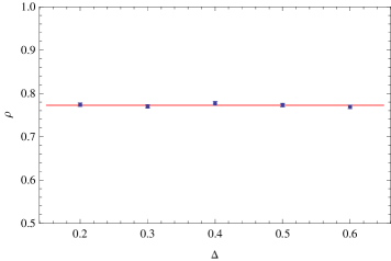
As is apparent from Fig. 6, bottom right, there is practically no dependence of on for fixed , despite the fact that the quality of the fits to the functional form (6) deteriorates for . On the other hand, leaving fixed and varying , the dependence becomes quite pronounced, with increasing monotonically as the A-C phase transition is approached. However, with the current data it is not really possible to nail down uniquely the functional form of the dependence, and thus the nature of the phase transition. Let us illustrate this point by drawing two different three-parameter fits through the data points of Fig. 6, bottom left. (Note that the error bars of the data points themselves are too small to be visible in the figure.) For fit 1 (red curve) we choose the form
| (10) |
for which we have determined the free parameters as
| (11) |
Given the excellent agreement with the data and the small error bars, one is tempted to conclude that the transition is characterized by a fractional critical exponent, a result which usually indicates a higher-order phase transition. However, such a conclusion would be premature. The error bars of such fits can be misleading, since they refer to a specific functional form, which is unlikely to be correct when we move away from the critical line. As an alternative, let us assume that is analytic in and goes to zero linearly as we approach the critical value , instead of with a fractional power. Matching the number of free parameters, the corresponding fit 2 (green curve) has the form
| (12) |
and its parameters have been determined as
| (13) |
corresponding to a critical value . We note that this fit is almost as good as the previous one (with rather than ), and the two curves are barely distinguishable on the plot. However, it leads to the rather different conclusion that the critical exponent is rather than , indicative of a first-order transition. The fact that the exponent lies more than 5 standard deviations away from reiterates our earlier assertion that the error bars given with the individual fits cannot be taken seriously as the only source of error. Deciding between these two possibilities will require taking data closer to the critical line, which is quite difficult from a simulation-technical point of view.
To summarize, the data presented above do not allow us to distinguish between a first- and a higher-order transition. The possibility of a higher-order A-C transition is intriguing, since it is exactly by changing that we encounter a transition scenario à la Kosterlitz-Thouless as described in the introduction, however, it is not supported by the results reported in [19]. There we observed an abrupt transition and clear evidence of a hysteresis when changing the coupling constants, which we interpreted as good evidence of a first-order transition. The results reported above do not really contradict this hypothesis, although they leave the door ajar to the possibility of a higher-order transition. More work is needed to settle this question decisively.
5 Effective action: curvature corrections
As mentioned above, the measured averaged volume distribution closely matches the behaviour of the same quantity derived from a discretized mini-superspace action. In [16], we made an effort to push this line of argument further by trying to determine the form of the effective action from measurements of the covariance matrix of the three-volume fluctuations . Extracting these data was more subtle, in part due to the presence of a zero-mode, whose origin was the constraint of keeping the number of (4,1)-simplices constant. This mode had to be projected out before one could invert the fluctuation matrix and use it to reconstruct an action. An unpleasant feature of this projection is its mixing of effects from the stalk with “bulk physics”. One new ingredient in the current work is to lift the constraint of a constant number of (4,1)-simplices, and thus avoid the zero-mode problem.
In this new setting, we study the covariance matrix and invert it to a matrix which in principle describes the (nonlocal) effective action resulting from fluctuations of the three-volume around the semiclassical solution (see [15] for details). Because we have added a term to the original Einstein-Hilbert action, each matrix element of receives a contribution . After subtracting this shift, we find that all matrix elements outside the diagonal and the neighbouring sub- and superdiagonals are zero up to numerical noise. To quadratic approximation in the fluctuations we have
| (14) |
Our observations then suggest that the effective action is quasi-local in time and can be expressed as
| (15) |
where the function and the potential need to be determined from the data and is an overall constant. The simplest function compatible with the observed scaling is
| (16) |
Assume now that the three-volume (equivalently, the third power of the scale factor of the universe) behaves according to
| (17) |
for some function , where denotes the location of an origin chosen along the discrete time axis. Comparing with (6), this scaling is consistent with our data and we have
| (18) |
where the last equality is required by normalization. Converting the function found in (16) to a continuum expression yields
| (19) |
where is a dimensionful time variable, and the lattice spacing in time direction.
We recognize (19) as the kinetic term of a minisuperspace action for a spatially homogeneous and isotropic universe. One could consider a variety of corrections to this term. More specifically, we are looking for corrections related to the short-distance behaviour of the theory. Taking guidance from the continuum theory of a homogeneous, isotropic universe with (Euclideanized) four-metric
| (20) |
the most general minisuperspace action containing both the Ricci scalar and a curvature-squared term999For a classical universe with metric (20), the a priori distinct terms , and in the action are all proportional. (the latter with coupling constant ), as well as a cosmological-constant term is of the form
| (21) |
We note the presence of fourth-order time derivatives, whereas the higher-order spatial derivatives in such a universe are converted to inverse powers of the scale factor . The -term multiplied by the inverse Newton constant in the integrand of (21) contains also a potential part , which in earlier work [16] was matched successfully to computer measurements. The fact that corresponding terms in the effective action (15) appear with the opposite sign compared to (20) has to do with nonperturbative contributions arising from integrating over the remaining degrees of freedom in the path integral [13, 14, 16, 21], and is therefore another feature of the nonperturbative nature of CDT’s semiclassical limit in phase C,
For the purposes of our present investigation, do we observe any trace of the terms contributing to the -term in our effective action? With regard to the purely diagonal potential term in (15), we would expect higher-order corrections101010Such a power expansion should be valid as long as does not become small, i.e. sufficiently far away from the “beginning” and “end” of the universe. in powers of , that is,
| (22) |
to the order we are considering, where the first term is a Lagrange multiplier term.111111From expression (22) it is clear that if the first two terms should both contribute to leading order in the continuum limit, at least one of the multiplying constants needs to scale nontrivially as a function of . This is borne out by relation (25) below. Next, let us turn to the kinetic term in . Since we have already seen that only nearest-neighbour terms contribute appreciably to the measured covariance matrix, we can immediately conclude that a term corresponding to – whose natural discretization would contain a term like , and therefore next-to-nearest-neighbour interactions – is absent. This is our first indication that in the region of phase space under investigation, there is no appreciable contribution from a squared-curvature term matching the one in the continuum expression (21), when re-expressed as function of the three-volume .
Let us look at another kinetic term expected to contribute to the action at this order, , to illustrate how a more quantitative analysis needs to proceed and what the potential implications are for the continuum limit of the theory, if we manage to construct one. Pretending for the time being that this term is the only correction to the finite-difference expression (16) at this order leads to a modified ansatz
| (23) |
As mentioned earlier, the higher-derivative expansion takes the form of a power series in or, equivalently, in inverse powers of the square root of the discrete four-volume (the number of four-simplices). It is our task to determine from the data whether or not such subleading terms are present in the effective action. However, let us emphasize that the presence of higher-derivative corrections at the regularized level, like those associated with the coefficients and in (22) and (23), does not imply that such terms necessarily survive in the continuum limit. For example, if in the simulations we observed a coefficient which was independent of the four-volume of the universe, we could convert the dependence on of the corresponding term in the action into a dependence on the lattice spacings and in the time and spatial directions according to
| (24) |
or in shorthand notation121212The notation “” for a generic lattice spacing should not be confused with the same notation for the scale factor .. In this case the term in (23) would be proportional to and simply drop out in a standard scaling limit where we keep constant while taking to infinity and the lattice spacings and to zero. Likewise, if we wanted to add such a higher-derivative term by hand already in the bare action, such that it survived in the classical limit, we would need to assume an appropriate nontrivial lattice dependence of the coefficient in front of the discretized higher-derivative term. However, we will not follow this latter route in the present work. This does not imply that no higher-curvature terms may appear in the effective action, it only means that no tunable coupling constant is associated with such terms, and that the coefficient is determined purely from the entropy of microstates.
In the region where we can presently perform reliable measurements, does not display any significant scale dependence. However, it could in principle pick up such a dependence when we move closer to a potential ultraviolet fixed point by changing the bare coupling constants, along the lines described in [16]. In this way, in the vicinity of a nontrivial ultraviolet fixed point (in principle infinitely many) higher-derivative terms can play a role. In view of this situation our task is to first identify potential higher-derivative terms in the effective action, and then study the scaling behaviour of the associated coupling constants.
Let us determine the effect of the presence of a -dependent term on the fluctuation matrix . We can use the fact that our tentative discretized action should reproduce the “observed” of (18) as an extremum. Extremality is satisfied if
| (25) |
To this order the result does not depend on the parameters and . Note that can be fully determined from the data for . Furthermore, the additional term proportional to gives no contribution to the classical solution, since the bare cosmological constant was chosen to achieve exactly that, as explained at the end of Sec. 2.
We can now use (15) to derive a prediction for the inverse covariance matrix, namely, the matrix of second derivatives at (see (14)), provided that the fluctuations around can be approximated by working up to second order in the (see [16] for a detailed discussion). It is a simple exercise to show that the matrix elements (after again eliminating a constant -shift) satisfy
| (26) |
where
| (27) |
As long as we keep only the leading term in (27), the right-hand side of (26) is independent of . However, the elements and can (and do) depend on at this order, provided these contributions cancel on the left-hand side of (26).
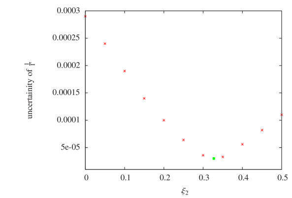
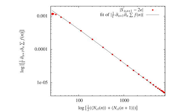
This is illustrated by the expression for , which after subtraction of a -contribution is given by
| (28) |
In Fig. 7 we compare this prediction with the data for the standard choice of bare constants. Notice that the term proportional to is with respect to the leading term, exactly as in the “potential” . Fig. 7 shows the results of the analysis including the leading correction to the kinetic term. The best fit is obtained for . This concludes our discussion of how to search for and analyze higher-order correction terms to the effective action. For such terms to have a continuum interpretation as a curvature-squared contribution like in the continuum action (21), we need to show that a whole bunch of coupling constants like exhibit the correct scaling behaviour as we follow their flow when we approach the critical phase transition lines. Our present Monte Carlo algorithm still needs improvement to deal with the critical slowdown appearing close to the B-C transition line, which in this context has our primary interest [16, 10].
In the appendix we repeat the above analysis for the system with subdivided time steps, analogous to what we did in Sec. 4 for the volume distribution. This turns out to be self-consistent, in the sense that integrating out the substructure at the discretized level produces a result compatible with what was derived for integer time steps in the present section.
6 Summary and discussion
In the work presented above, we have analyzed several properties of the semiclassical limit of CDT quantum gravity, a limit which is inherently nonperturbative in nature. We used a modified simulation method which replaces the fixing of the total four-volume to a specific value by a Gaussian distribution peaked at . In this way one avoids the presence of a zero-mode of the volume fluctuations, whose removal had hampered the extraction of short-distance continuum physics in previous work.
After reconfirming our previous result for the de Sitter volume profile we measured the probability distributions for finding a three-volume at a fixed, given time step . Well inside the universe, we found them to be Gaussian around the average, confirming their semiclassical nature. Moving toward the ‘stalk’, where becomes small, the probability distributions become asymmetric and display discretization artifacts, in the sense that the data in each can be seen to separate into three distinct families. These effects are confined to very small length scales, but – depending on the type of observable under study – they can potentially interfere with the nonperturbative physical short-distance effects we are keen to explore, for example, along the lines suggested in [24].
The volume profile is an example of an observable which is not particularly sensitive to these discretization artifacts, even down to short scales. We found further evidence for this remarkable robustness when refining our spatial slicing, effectively doubling the number of slices in a given time interval. This was done by identifying the connected (on the dual lattice) layers of (3,2)-simplices in between successive (4,1)-layers with slices of fixed half-integer time. Determining the volume profile for the (3,2)-layers alone, we found that after rescaling their volume by a constant , the resulting profile could be combined with the previous data for the (4,1)-slices to yield a single, universal volume distribution. This analysis could be extended further by splitting each time interval not just into two but into three, yielding a similar outcome. Our results show that the macroscopic geometry associated with the semiclassical limit of CDT quantum gravity is not closely linked to the microscopic piecewise linear geometry of the building blocks, in line with the nonperturbative character of this limit. Our attempt to learn more about the nature of the A-C phase transition by studying the scaling behaviour of the constant as a function of the bare parameters and yielded at this stage inconclusive results.
Our new method of volume-fixing also enabled us to make new precision measurements of the effective action for the three-volume fluctuations of the universe around its semiclassical limit. Specifically, we investigated correction terms to the action – obtained by inverting the covariance matrix – which are of higher order in powers of and are associated with curvature-squared terms in the continuum. We observed nonvanishing correction terms of this type in the discretized action, while others, expected from a comparison with the continuum, gave little or no contribution. This neither proves nor disproves the presence of higher-order curvature terms, since we found that their coefficients in the discrete effective action must have a specific, nontrivial scaling behaviour (as a function of the UV cut-off ) in order to survive in the limit . We undertook a careful, quantitative analysis of one of these coefficients, but did not find evidence for the required scaling, at least not for the range of coupling constants considered. The implication is that there is currently no evidence for the presence of higher-order curvature in CDT quantum gravity, although this issue needs to be re-examined once we have improved our algorithms to penetrate to shorter distance scales by performing the simulations closer to the putative UV fixed points in the phase diagram.
Acknowledgements. This work is partly supported by the International PhD Projects Programme of the Foundation for Polish Science within the European Regional Development Fund of the European Union, agreement no. MPD/2009/6. AG and JJ ackonowledge a partial support by the Polish Ministry of Science grant N N202 229137 (2009-2012).
Appendix
In this appendix, we repeat the analysis of Sec. 5 for the system where we have subdivided all time steps into two, as already described in Sec. 4. That is, we associate constant half-(odd-)integer times to the layers made up of - and -simplices. We want to investigate whether this finer-grained system can also be described by a discretized semiclassical effective action. If so, the action we have already derived, based on the data from integer-valued constant-time slices alone should be obtainable from the new effective action by integrating out the - and -“degrees of freedom”. In this way the system described by the integer-time slicing may be understood as arising from a “Kadanoff blocking” in time of the larger, finer-grained system.
After measuring the covariance matrix of “three-volume” fluctuations131313We put “three-volume” in quotation marks because – unlike the number of (4,1)-simplices – the number of (3,2)- and (2,3)-simplices in a slab between times and does not have a direct interpretation in terms of a three-volume. for all integer and half-integer times, we invert this matrix to obtain the effective action, up to quadratic terms in the fluctuations. The large inverted covariance matrix can be decomposed into blocks describing the (4,1)-system (at integer time), the (3,2)+(2,3)-system (at half-integer times) and off-diagonal blocks describing interactions between the two. As expected, we observe a constant shift by in the (4,1)-block only, which we subtract from the entries of the fluctuation matrix.
The functional form of the matrix entries resembles that found in Sec. 5, but with some modifications. Before proceeding further, let us rescale the number of (3,2)+(2,3)-vertices with the factor determined in Sec. 4 to obtain the number which is part of the universal volume distribution , valid for both integer and half-integer . The measured matrix structure is consistent with an effective action of the form
where
| (30) | |||||
and
| (31) | ||||
We observe that the “kinetic”, finite-difference terms couple not only neighbouring layers (in this case and ), but also directly the (4,1)-layers at to those at , in the latter case with a negative sign. We have checked that this feature persists when we perform a further “time refinement” by associating the (3,2)- and (2,3)-simplices with distinct spatial slices, as was done in Sec. 4 above. There are further unexpected minus-signs in the potential , and a new correction term linear in in the kinetic term . We take this as an indication that – unlike what happened in our earlier analysis of the volume distribution itself – we run into short-distance lattice artifacts for measurements of the volume fluctuations when considering the subdivided slicings.
Demanding that integrating over the (3,2)-fluctuations should give back the (4,1)-effective action leads to explicit relations among , , , as well as among , , and , , . A simple, but tedious computation yields
| (32) |
and
| (33) | |||||
as well as relations between , and .
We have checked numerically that starting out with the larger covariance matrix of the subdivided system and integrating out the (3,2)-fluctuations reproduces within measuring accuracy the covariance matrix determined earlier by considering integer times only. The results at the point in phase C are presented in the table below, which compares the directly measured
| parameter | direct | integrated |
|---|---|---|
| (from (4,1)) | (from (4,1) and (3,2)) | |
parameters of the (4,1)-action (15) with their counterparts obtained from measuring the fine-grained system and using formulae (32) and (33). In the fits we have neglect higher-order corrections, and the errors are estimated as statistical errors of the fits. In view of this the agreement between the two sets of values appears quite satisfactory.
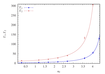
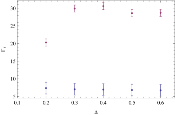
We have also examined the dependence of the action parameters on the bare coupling constants, using the same values as in the analogous investigation of the parameter in Sec. 4. For constant we observe a marked dependence on (see Fig. 8), in the sense that both and seem to diverge when approaching the critical line for the A-C phase transition. For fixed we observe a nontrivial behaviour of , which may be corroborating evidence that the semiclassical scaling function (6) ceases to give a good description of the three-volume distribution around .
References
-
[1]
A. Codello, R. Percacci and C. Rahmede:
Investigating the ultraviolet properties of gravity with a Wilsonian
renormalization group equation,
Annals Phys. 324 (2009) 414,
arXiv:0805.2909 [hep-th].
E. Manrique, M. Reuter and F. Saueressig: Bimetric renormalization group flows in Quantum Einstein Gravity, Annals Phys. 326 (2011) 463-485, arXiv:1006.0099 [hep-th].
J.E. Daum, U. Harst and M. Reuter: Running gauge coupling in asymptotically safe quantum gravity, JHEP 1001 (2010) 084, arXiv:0910.4938 [hep-th].
M. Reuter and F. Saueressig: Functional renormalization group equations, asymptotic safety, and Quantum Einstein Gravity arXiv:0708.1317 [hep-th];
M. Niedermaier and M. Reuter: The asymptotic safety scenario in quantum gravity, Living Rev. Rel. 9 (2006) 5;
H.W. Hamber and R.M. Williams: Nonlocal effective gravitational field equations and the running of Newton’s G, Phys. Rev. D 72 (2005) 044026 [hep-th/0507017];
D.F. Litim: Fixed points of quantum gravity, Phys. Rev. Lett. 92 (2004) 201301 [hep-th/0312114];
H. Kawai, Y. Kitazawa and M. Ninomiya: Renormalizability of quantum gravity near two dimensions, Nucl. Phys. B 467 (1996) 313-331 [hep-th/9511217]. - [2] S. Weinberg: Ultraviolet divergences in quantum theories of gravitation, in General relativity: Einstein centenary survey, eds. S.W. Hawking and W. Israel, Cambridge University Press, Cambridge, UK (1979) 790-831.
- [3] P. Hořava: Quantum gravity at a Lifshitz point, Phys. Rev. D 79 (2009) 084008 arXiv:0901.3775 [hep-th].
-
[4]
J. Ambjørn, J. Jurkiewicz and R. Loll:
A non-perturbative Lorentzian path integral for gravity,
Phys. Rev. Lett. 85 (2000) 924
[hep-th/0002050];
Dynamically triangulating Lorentzian quantum gravity, Nucl. Phys. B 610 (2001) 347-382 [hep-th/0105267]. - [5] J. Ambjørn and J. Jurkiewicz, Four-dimensional simplicial quantum gravity, Phys. Lett. B 278 (1992) 42.
-
[6]
C. Teitelboim:
Causality versus gauge invariance in quantum gravity and supergravity,
Phys. Rev. Lett. 50 (1983) 705-708;
The proper time gauge in quantum theory of gravitation, Phys. Rev. D 28 (1983) 297-309. - [7] J. Ambjørn, J. Jurkiewicz and R. Loll: Spectral dimension of the universe, Phys. Rev. Lett. 95 (2005) 171301 [hep-th/0505113].
- [8] O. Lauscher and M. Reuter: Fractal spacetime structure in asymptotically safe gravity, JHEP 0510 (2005) 050 [arXiv:hep-th/0508202].
- [9] P. Hořava: Spectral dimension of the universe in quantum gravity at a Lifshitz point, Phys. Rev. Lett. 102 (2009) 161301, arXiv:0902.3657 [hep-th].
- [10] J. Ambjørn, A. Görlich, S. Jordan, J. Jurkiewicz and R. Loll: CDT meets Hořava-Lifshitz gravity, Phys. Lett. B 690 (2010) 413-419, arXiv:1002.3298 [hep-th].
- [11] P. Hořava: General covariance in gravity at a Lifshitz point, arXiv:1101.1081 [hep-th].
- [12] J. Ambjørn, J. Jurkiewicz and R. Loll: Emergence of a 4D world from causal quantum gravity, Phys. Rev. Lett. 93 (2004) 131301, 4 pages [hep-th/0404156].
- [13] J. Ambjørn, J. Jurkiewicz and R. Loll: Reconstructing the universe, Phys. Rev. D 72 (2005) 064014, 24 pages [hep-th/0505154].
- [14] J. Ambjørn, J. Jurkiewicz and R. Loll: Semiclassical universe from first principles, Phys. Lett. B 607 (2005) 205-213 [hep-th/0411152].
- [15] J. Ambjørn, A. Görlich, J. Jurkiewicz and R. Loll: Planckian birth of the quantum de Sitter universe, Phys. Rev. Lett. 100 (2008) 091304, 4 pages, arXiv:0712.2485 [hep-th].
- [16] J. Ambjørn, A. Görlich, J. Jurkiewicz and R. Loll: The nonperturbative quantum de Sitter universe, Phys. Rev. D 78 (2008) 063544, 17 pages, arXiv:0807.4481 [hep-th].
-
[17]
J. Ambjørn, J. Jurkiewicz and R. Loll:
The universe from scratch,
Contemp. Phys. 47 (2006) 103-117 [hep-th/0509010];
R. Loll: The emergence of spacetime, or, quantum gravity on your desktop, Class. Quant. Grav. 25 (2008) 114006, arXiv:0711.0273 [gr-qc]. -
[18]
J. Zinn-Justin:
Quantum field theory and critical phenomena,
Int. Ser. Monogr. Phys. 113 (2002) 1. - [19] J. Ambjørn, A. Görlich, S. Jordan, J. Jurkiewicz and R. Loll: CDT meets Horava-Lifshitz gravity, Phys. Lett. B 690 (2010) 413-419, arXiv:1002.3298 [hep-th].
- [20] J. Ambjørn and R. Loll: Non-perturbative Lorentzian quantum gravity, causality and topology change, Nucl. Phys. B 536 (1998) 407-434 [hep-th/9805108].
- [21] J. Ambjørn, J. Jurkiewicz and R. Loll: Quantum gravity as sum over spacetimes, Lect. Notes Phys. 807 (2010) 59-124, arXiv:0906.3947 [gr-qc].
- [22] T. Regge: General relativity without coordinates, Nuovo Cim. 19 (1961) 558.
- [23] A. Dasgupta and R. Loll: A proper time cure for the conformal sickness in quantum gravity, Nucl. Phys. B 606 (2001) 357-379 [hep-th/0103186].
- [24] J.E. Daum, U. Harst and M. Reuter: Running gauge coupling in asymptotically safe quantum gravity, JHEP 1001 (2010) 084, arXiv:0910.4938 [hep-th].