A dynamic hybrid model based on wavelet and fuzzy regression for time series estimation

Abstract

In the present paper, a fuzzy logic based method is combined with wavelet decomposition to develop a step-by-step dynamic hybrid model for the estimation of financial time series. Empirical tests on fuzzy regression, wavelet decomposition as well as the new hybrid model are conducted on the well known $SP500$ index financial time series. The empirical tests show an efficiency of the hybrid model.

1 Introduction

The study of time series is an interesting task especially in financial contexts such as modeling, estimating, approximating and prediction. It necessitates a precise and deep comprehension of the series characteristics for a suitable choice of the model to be applied. The estimation process guarantees the detection of passed disfunction causes and therefore, it helps to take the eventual and possible precautions at the suitable time. A fine and preventive analysis guarantees a good preparation for the future and a robust prediction in front of random breaks and non anticipated changes. Financial time series are for example, are characterized by very specific stylized facts where a respect with estimation method proves its efficiency. Observing the distribution tail, for the leptokurtic cases always evaluated by the kurtosis, the series values far from the mean of the series appears with probabilities that overcome the normal distribution. In financial case, the studies have shown that the tail distribution is not leptokurtic but in the contrary, it has a kurtosis exceeds the normal case. Furthermore, observing the volatility clustering, financial time series are characterized by complex combinations of components with high frequencies. These facts are somehow due to the presence of the random or stochastic behavior of the markets. Besides, the market may be characterized by infinite volatility allowing long memory process. This induces the appearing of scaling law invariance on the volatility (Walter, 2001). Indeed, Walter expects that the conciliation between absence of long memory on profitability and its presence on volatility is a modeling financial problem. Due to these facts, some classical methods have been classified as incapable to analyze financial series. ARCH and GARCH models did not take into account the kurtosis degree of the series. Furthermore, ARCH model and its terminologies have attained their limits in the field of financial modeling due to the fact that the scaling law in volatility has not been included in the model. (See also Walter, 2001). For this aim, researchers in financial time series field have thought to introduce other methods that may induce more efficient models and to understand some aspects of non stationary, auto-regression, filtering, support vector machine models and prediction, neural networks models and predicting. See (Angue, 2007), (Azizieh, 2002), (Ben Mabrouk et al 2008a,b), (Ben Mabrouk et al 2008), (Ben Mabrouk et al 2010), (Ben Mabrouk et al, 2011), (Chang et al, 2001), (Chen et al, 2006), (Chou, 2005), (Klir et al, 1995), (He et al, 2007), (Khashei et al, 2008), (Kim et al, 1996), (Mitra et al, 2004), (Podobnik et al, 2004), (Ramsey, 1999), (Struzik, 2000), (Tanaka et al, 1982), (Tseng et al, 1999), (Tseng et al, 2001), (Wang et al, 2000), (Watada, 1992), (Wu et al,2002), (Zopoundis et al, 2001).

In the present paper, one aim is to apply wavelet theory and fuzzy logic theory to develop an estimation model for financial series. We search to judge the efficiency of fuzzy regression to estimate financial series. Next, we apply the discrete wavelet decomposition which improve especially the study of the local behavior of the series. Comparing the two methods of estimation, we have discovered that an hybrid model combining wavelet estimation with fuzzy logic estimation is possible. We then developed such a model which takes into account the non stationary behavior of the series as well as its local fluctuations and its fuzzy characteristics. The model combines wavelet decomposition with fuzzy regression. Next, an empirical study based on the famous $SP500$ index is provided in order to improve the theoretical parts.

The present paper is organized as follows. A first section is devoted to the presentation of the series characteristics. Section 2 is devoted to the development of the fuzzy regression model for the estimation of financial time series. In section 3, a wavelet analysis of time series is provided. In section 4, the hybrid model deduced by combining fuzzy logic with wavelet decomposition is developed. Finally, an empirical study on the SP500 index is developed in section 5 leading to a comparison between the different models and improving the impact of the hybrid scheme.

2 The Data Description

In the present paper, we propose to study the behavior of the well known financial index $SP500$ which is a stock index describing the fluctuations of the stock capitalization due to the 500 most large economic societies of the American stock. It is composed of a number of 380 industrial firms, 73 financial societies, 37 public service firms, and 10 transport ones. The choice of such an index is motivated essentially by its central role as a measure of the American economy performance. Besides, the international financial integration is often increasing which forces the international exchanged productions to be strongly related. So that, as the American market is the center of international transactions, any variation of its index such as $SP500$ immediately affects on other external markets. Furthermore, the study of the USA market index is of interest nowadays due to the financial international crisis which has been started from this market and next affected the world-wise markets. So, searching a good solution to understand the crisis is of priority.

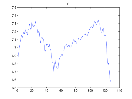
The data basis consists of $SP500$ index monthly values during the period from August 1998 to March 2009 allowing a basis of size $N=128=2^{7}$. We applied the $\log$-values of the series in order to reduce the range of the series. The statistic characteristics of the series are resumed in the following table.

Sample size, $N=$	128
Mean	7.0921
Variance	0.0246
Maximum	7.3456
Minimum	6.6000
Kurtosis	3.2229
skewness	-0.9017

Table 1: Statistic Characteristics

We notice a kurtosis value over-crossing the normal value 3 which means that the series is leptokurtic. The skewness of the series induces a negative value which means that the data are spread out more to the left relatively to the means of the series than to the right. The following figure represents the original series $S(t)=\log(SP(t))$, where $SP(t)$ is the corresponding value of the index $SP500$ at the month $t$.

Figure 1: Original Series $S(t)$

3 A fuzzy regression model

The reasons behind the test of fuzzy regression for modeling financial series has many justifications. Firstly, financial series have always an ambiguous relation concerning dependent variables and independent one; The time variable here. Such an ambiguity is not taken into account in almost all statistical methods, but in the contrary they assume that the behavior is always definite. Furthermore, financial series such as $SP500$ are already fluctuated with an unpredicted behavior. This permanence makes the future values of the series to be fuzzy and/or imprecise. The fuzzy regression was already applied as a privileged method for the estimation of uncertain and imprecise data. See (He et al, 2007), (Khashei et al, 2008), (Kim et al, 1996), (Sanchez et al, 2003), (Shapiro, 2005), (Terence, 1999), (Tseng et al, 1999), (Tseng et al, 2001), (Watada, 1992), (Wu et al, 2002), (Zopoundis et al, 2001).

In this section, a fuzzy regression model is applied to estimation the $SP500$ index series. The model due to Watada 1992, is applied here. This model is reviewed hereafter. It is based on the following fuzzy linear programming.

$$\left\{\matrix{\vskip 6.0pt plus 2.0pt minus 2.0pt\,MinS=s_{0}+s_{1}\hfill\cr\vskip 6.0pt plus 2.0pt minus 2.0pts.t\hfill\cr\vskip 6.0pt plus 2.0pt minus 2.0ptc_{0}+c_{1}t_{i}-(1-h)(s_{0}+s_{1}|t_{i}|)\leq Y_{i},\hfill\cr\vskip 6.0pt plus 2.0pt minus 2.0ptc_{0}+c_{1}t_{i}+(1-h)(s_{0}+s_{1}|t_{i}|)\geq Y_{i},\hfill\cr\vskip 6.0pt plus 2.0pt minus 2.0pts_{j}\geq 0\quad and\quad s_{1}\geq 0,\hfill\cr\vskip 6.0pt plus 2.0pt minus 2.0pt\forall t_{i}=1,...,128.\hfill}\right.$$ (1)

where

• $h$ is a standard threshold, hereafter applied for $h=0.5$.

• $a_{j}=(c_{j},s_{j})$, $(j=0,1)$ is a triangular fuzzy number.

• $t_{i}$ is the time variable.

• $Y_{i}$ is the observed index value at the time $t_{i}$, $i=1,\dot{,}128$.

The problem is resolved using the Software LINGO9 resulting in the following fuzzy coefficients (Triangular fuzzy numbers).

$$a_{0}=(6.887995,0)\quad\hbox{and}\quad\,a_{1}=(0.01066521,0.06912872).$$ (2)

As a result the lower and upper estimations of the index series is provides resulting in the following fuzzy regression equation.

$$Y_{i}=(6.887995,0)+(0.01066521,0.06912872)*0,5*t_{i}.$$ (3)

The original series with its fuzzy estimation are shown in the Figure 2 following.

Figure 2: Original series and its fuzzy regression estimation

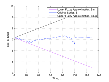
We notice that although the fuzzy regression model takes into account the uncertain behavior of the information, it did not fits well the tendency of the series, and it assumes that a monotone behavior exists which means that it ignores the fluctuations already characterizing the data. Besides, the error estimation is important resulting in the values

$$MSE=5.31016565\quad\hbox{and}\quad RMSE=2.30437967$$

where

$$MSE=\sum_{i}{(Y_{i}-\widehat{Y_{i}})^{2}/128}\quad i=1,...,128,$$ (4)

$$RMSE=\sqrt{MSE},$$ (5)

and $\widehat{Y_{i}}$ is the estimated value of the index at the time $t_{i};\,i=1,...,128$.

As a conclusion, the fuzzy regression has been proved to be incapable for a robust estimation with a least error for the series applied. It necessitates to be corrected to fit the fluctuations and then the random behavior of the series. So, an analysis permitting to localize these fluctuations is necessary. It consists of wavelet analysis which will be developed in the next section.

4 Wavelet analysis of the series

Wavelet analysis is always applied to show how the series is volatile, and then to detect eventual fluctuations, (Patick, 2005). Wavelet analysis permits also to represent the strongly fluctuated series without necessitating a knowledge of the explicit functional dependence. Such a capacity is of great role especially for financial time series where such a dependence is always unknown.

We propose hereafter to conduct a wavelet analysis of the series due to the index $SP500$ in order to localize well the fluctuations of the series. A maximum level decomposition $J=6$ is fixed allowing a decomposition or a projection on the approximation space $V_{6}$ relatively to a Daubechies $DB4$ multi-resolution analysis with Matlab7 software.

As a result the series $S(t)$ is decomposed on the form

$$S=(A_{6},\quad D_{1},\quad D_{2},\quad D_{3},\quad D_{4},\quad D_{5},\quad D_{6})$$

or equivalently,

$$S=D_{1}+D_{2}+D_{3}+D_{4}+D_{5}+D_{6}+A6$$

where $A_{6}$ is the global form of $S(t)$ at the level $6$ called also the trend or tendency, and $D_{1}$, $D_{2}$, $D_{3}$, $D_{4}$, $D_{5}$ and $D_{6}$ are the detail components of $S(t)$ obtained by projecting the series on the detail spaces $W_{1}$, $W_{2}$, $W_{3}$, $W_{4}$, $W_{5}$ and $W_{6}$. These components are represented hereafter.

Figure 3: Approximation $A_{6}$

Figure 4: Detail component $D_{6}$

Figure 5: Detail component $D_{5}$

Figure 6: Detail component $D_{4}$

Figure 7: Detail component $D_{3}$

Figure 8: Detail component $D_{2}$

Figure 9: Detail component $D_{1}$

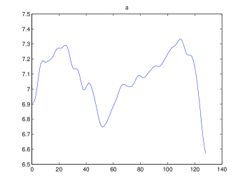
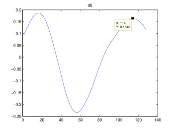
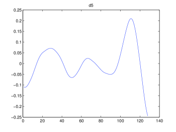
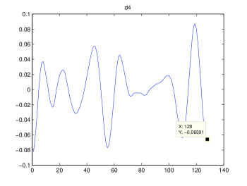
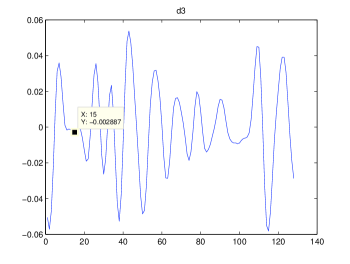
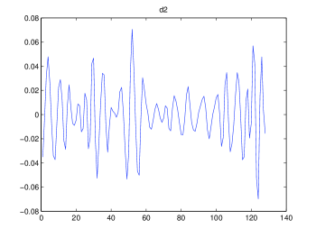
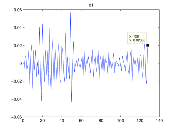
We notice easily from these figures the localizations of the fluctuations of the series. The component $A_{6}$ shows the low frequency fluctuations. The components $D_{i}$, $i=1,2,...,6$ represents the high frequency behavior. We remark that the series is more fluctuated at detail levels $D_{4}$ and $D_{3}$ more than $D_{5}$ and $D_{6}$. The volatile aspect of the series is clearly observed from $D_{1}$ and $D_{2}$.

5 Hybrid estimation model

As we have localized the fluctuations of the series, we propose to return to the fuzzy regression model and to conduct a correction on it consisting in re-developing a dynamic fuzzy regression taking into account both the fluctuations and the uncertain aspect of the series. Denote $S(t)$ the financial time series due to the $SP500$ index introduced previously. The proposed hybrid model is described by the following steps.

• Step 1: The wavelet decomposition of the series; ($D_{1}$,$D_{2}$,$D_{3}$,$D_{4}$,$D_{5}$,$D_{6}$,$A_{6}$).

• Step 2: Compute the localizations of the extremum points of each component $D_{i}$; $i=1,2,...,6$.

• Step 3: Apply the fuzzy regression to estimate the restriction of the series on each interval $[t_{n}(i),t_{n+1}(i)]$ where $t_{n}(i)$, $t_{n+1}(i)$ are two consecutive extremum points for the component $D_{i}$; $i=1,2,...,6$.

• Step 4: For all $i=1,2,...,6$, regroup the new series obtained on the whole time interval $\displaystyle\bigcup_{n}[t_{n}(i),t_{n+1}(i)]$.

We remark easily that the proposed model fits the peace-wise monotonicity of the time series. On each interval, where the series is monotone the fuzzy regression is applied with corresponding fuzzy numbers. The results due to this model are shown in following figures.

Figure 10: Estimation relatively to $D_{6}$.

Figure 11: Estimation relatively to $D_{5}$.

Figure 12: Estimation relatively to $D_{4}$.

Figure 13: Estimation relatively to $D_{3}$.

Figure 14: Estimation relatively to $D_{2}$.

Figure 15: Estimation relatively to $D_{1}$.

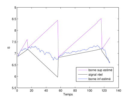
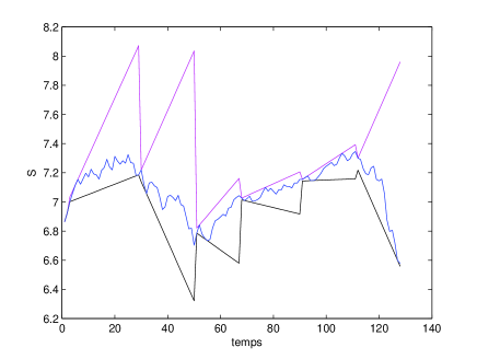
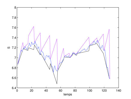
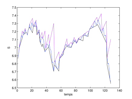
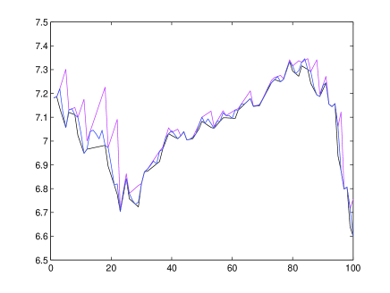
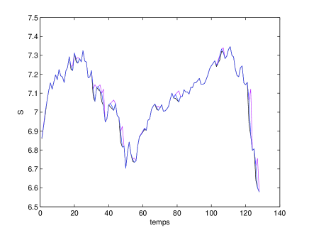
As we see, the new estimation due to the hybrid model fits more the original series as the detail level decreases. Here, we stress the fact that Daubechies wavelets in the software Matlab7 uses the frequency index $-j$ contrarily to the theoretical way of wavelet basis definition which uses instead the index $j$. So, we seek here an increasing in the detail approximation as $j$ decreases. Indeed, the estimation relatively to $D_{6}$ is somehow abusive (See Figure 10). This is due to the fact this component does not contain an important number of extremum points or fluctuations. The estimation becomes more efficient when using $D_{5}$ (See Figure 10). Next, Figures 12, 13, 14, 15 show an increasing in the fitness between the original series and the hybrid model estimated one. This is due to the fact that the hybrid model follows well the fluctuations of the series. To finish with this model, we provided in the following table the different error estimates corresponding to the details $D_{i}$; $i=1,2,...,6$.

The model	MSE	RMSE
Fuzzy Regression	1.5380	1.2401
Hybrid with $D_{6}$	0.4100061	0.64032
Hybrid with $D_{5}$	0.1506692	0.380324
Hybrid with $D_{4}$	0.0402139	0.2006
Hybrid with $D_{3}$	0.01133175	0.1064507
Hybrid with $D_{2}$	0.00261067	0.0611
Hybrid with $D_{1}$	0.00060889	0.024675

Table 2: Error estimates

6 Conclusion

In the present paper, a fuzzy regression estimation is applied to estimate financial time series. Such estimation is shown to be not efficient. It gives an estimation with affine boundaries to the series which did not follow the fluctuations well. As financial time series are very volatile, a wavelet decomposition is applied next to localize the fluctuations and then to prepare to a more sophisticated fuzzy model taking into account the fluctuations. As a result, an hybrid model combining fuzzy regression and wavelet decomposition is developed. Finally, the different models are tested on the well known financial time series of the $SP500$ index. The empirical tests show an efficiency of the hybrid model. We intend in the future to apply the hybrid method or modified versions for other time series and for prediction aims.

References

- [1] Angue K. (2007), Régression floue: principes et applications en sciences de gestion. Université de Nice Antipolis, Laboratoire Gredge, Preprint.
- [2] Azizieh C. (2002), Modélisation de séries financières par un modèle multifractal. Mémoire pour diplôme d’actuaire. Université Libre de Bruxelles.
- [3] Ben Mabrouk A., Ben Abdellah N. and Dhifaoui Z. (2008a), Wavelet decomposition and autoregressive model for time series prediction. Applied Mathematics and computation, 199, 334-340.
- [4] Ben Mabrouk A., Dhifaoui Z. and Kortas H., (2008b), A wavelet support vector machine coupled method for time series prediction. International Journal of Wavelets Multiresolution and Information Processing, 6(6) (2008), 851-868.
- [5] Ben Mabrouk A., Kortas H. and Ben Ammou S., (2009), Wavelet estimators for long memory in stock markets. International J. of Theoretical and Applied Finance 12(3) (2009), 297-317.
- [6] Ben Mabrouk A., Kahloul I. and Hallara S., (2010), Wavelet-Based Prediction for Governance, Diversification and Value Creation Variables. IRJFE, 60 (2010), 15-28.
- [7] A. Ben Mabrouk, N. Ben Abdallah and M. Essaied Hamrita, (2011), A wavelet method coupled with quasi self similar stochastic processes for time series approximation. Interna. J. Wavelets Multires. Information Processing, To appear.
- [8] Chang H-S. O. and Ayyub B. M. (2001), Fuzzy regression methods: a comparative assessment. Fuzzy Sets and Systems, 119, 187-203.
- [9] Chen Y., Yang B. and Dong J. (2006), Time-series prediction using a local wavelet neural network. Neurocomputing, 69, 449-465.
- [10] Chevrie F. et Guely F. (1998), La logique floue, Cahier Technique n 191. Collection Technique. Edition Shneider.
- [11] Chou R. Y. (2005), Forecasting financial volatilities with extreme values: the conditional autoregressive Range (CARR) model. Journal of money, credit, and banking, 37(3), 561-582.
- [12] Chyu C. L. U. and Chiang K. (2002), A Fuzzy linear regression model with better explanatory power. Fuzzy Sets and Systems, 126, 401-409.
- [13] Daubechies I. (1992), Ten lectures on wavelets. Society for Industrial and Applied Mathematics, Philadelphia, PA, USA.
- [14] Klir G. J. and Yuan B. (1995), Fuzzy sets and fuzzy logic: theory and applications. Prentice Hall.
- [15] He Y. Q., Chan L. K. and Wu M. L. (2007), Balancing productivity and consumer satisfaction for profitability: statistical and fuzzy regression analysis. European Journal of Operational Research, 176, 252-263.
- [16] Khashei M., Hejazi S. R. and Bijari M. (2008), A new hybrid artificiel neural networks and fuzzy regression model for time series forecasting. Fuzzy Sets and Systems, 158, 769-786.
- [17] Kim K. J., Moskotwiz H. and Kosksalam M.(1996), Theory and methodology: fuzzy versus statistical linear regression. European Journal of Operational Research, 92, 417-434.
- [18] Missiti M., Missiti Y., Oppenheim G. and Poggi. J. M (2002), Wavelet toolbox for use with Matlab. The MathWorks, Inc., Version 2.
- [19] Mitra A. and Mitra S. (2004), Forecasting business cycle mouvements using wavelets filtering and neural networks. Finance India, 18, 1605-1626.
- [20] Podobnik B., Ivanov P. Ch, Grosse I., Matia K. and Stenley H. E. (2004), ARCH-GARCH approches to modeling high frenquency financial data. Physica A, 344, 216-220.
- [21] Ramsey J. B. (1999), The contribution of wavelets to the analysis of economic and financial data. Phil. Trans. R. Soc. Lond. A, 357, 2593-2606.
- [22] Sanchez J. and Gomez T. (2003), Application of fuzzy regression in actuarial analysis. The Journal of Risk and Insurance, 70(4), 665-699.
- [23] Sanchez J. A. (2006), Calculating insurance claim reserves with fuzzy regression. Fuzzy Sets Systems, 157, 3091-3108.
- [24] Struzik Z. R. (2000), Wavelets methods in financial time series processing. Information system, ……
- [25] Tanaka U., Ujema S. and Asai K.(1982), Linear regression analysis with fuzzy models. IEEE Transactions on Systems Man and Cybernetics, 12(6), 903-907.
- [26] Tseng F., Tzeng G. , Yu H. C. and Yuana B. J. C. (1999), Fuzzy seasonal time series for forecasting the production value to the mechanical industry in Taiwan. Technological Forecasting and Social Change, 60, 263-273.
- [27] Tseng F., Tzeng G., Yu H. C. and Yuana B. J. C. (2001), Fuzzy ARIMA model for forecasting the foreign exchange market. Fuzzy Sets and Systems, 118, 9-19.
- [28] Walter C. (2001), Les échelles de temps sur les marchés financiers. Revue de Synthèse, 4(1), 55-69.
- [29] Wang H. F. and Tsaur R. C. (2000), Insight of a fuzzy regression model. Fuzzy Sets and Systems, 122, 335-369.
- [30] Watada J. (1992), Fuzzy time-series analysis and forecasting of sales volume. Fuzzy Regression Analysis, J. Kacprzyk and M. Fedrizzi (eds) Omnitech Press, Warsaw and Physica-Verlag, Heidelberg, 1992, 211-227.
- [31] Watada J., Imoto S. and Yabuchi Y. (2007), Fuzzy regression model of R and D Evaluation. Applied Soft Coumputing, 8, 1266-1273.
- [32] Wu B. and Tseng N. F. (2002), A new approach to fuzzy regression models with application to busisness cycle analysis. Fuzzy Sets and Systems, 130, 33-42.
- [33] Yen K. K., Ghoshary S. and Roig G. (1995), A linear regression model using triangular fuzzy number coefficients. Fuzzy Sets and Systems, 106, 167-177.
- [34] Zadeh L. A. (1965), Fuzzy sets. Information and Control, 8, 338-353.
- [35] Zadeh L. A. (1978), Fuzzy sets as a basis for a theory of possibility. Fuzzy Sets and Systems, 1, 3-28.
- [36] Zopoundis C., Pardalos P. M. and Baourdis G. (2001), Fuzzy sets in management, economics and marketing. World Scientific Publishing.