Generating Transition Paths by Langevin Bridges

Abstract

We propose a novel stochastic method to generate paths conditioned to start in an initial state and end in a given final state during a certain time $t_{f}$. These paths are weighted with a probability given by the overdamped Langevin dynamics. We show that these paths can be exactly generated by a non-local stochastic differential equation. In the limit of short times, we show that this complicated non-solvable equation can be simplified into an approximate stochastic differential equation. For longer times, the paths generated by this approximate equation can be reweighted to generate the correct statistics. In all cases, the paths generated by this equation are statistically independent and provide a representative sample of transition paths. In case the reaction takes place in a solvent (e.g. protein folding in water), the explicit solvent can be treated. The method is illustrated on the one-dimensional quartic oscillator.

I Introduction

The problem of finding the pathway of chemical or biological reactions is of utmost importance for the understanding of their underlying mechanisms, as it allows to have better control on these reactions 1 . For instance, in the realm of proteins, understanding the pathway between the unfolded state and the native state, or between two native states of the protein (allostery) may help prevent certain reactions or on the contrary favor them. Recent progress in single molecule experiments have allowed to monitor the spontaneous thermal folding and unfolding of single proteins, or the force induced unfolding of proteins 3 ; 4 ; 5 .

In the following, we will study the spontaneous or the driven transition between an initial state denoted A and a final state denoted B.

This problem has been addressed mainly by stochastic methods which start from an initial path and deform it by sampling the vicinity of the path. These are the path sampling methods 6 ; 7 ; 8 . The main drawback of these methods is that they are time consuming, and they generate strongly correlated trajectories. As a consequence, the space of sampled trajectories depends strongly on the initial used path. The same kind of problem exists for the Dominant Pathway method 9 ; 10 , where the minimal action path depends strongly on the initial guess.

From now on, we assume that the system is driven by stochastic dynamics in the form of an overdamped Langevin equation

$$\frac{dx}{dt}=-\frac{1}{\gamma}\frac{\partial U}{\partial x}+\eta(t)$$ (1)

For the sake of simplicity, we illustrate the method on a one-dimensional system, the generalization to higher dimensions or larger number of degrees of freedom being straightforward. In this equation, $x(t)$ is the position of a point at time $t$ in a potential $U(x)$, $\gamma$ is the friction coefficient, related to the diffusion constant $D$ through the relation $D=k_{B}T/\gamma$, where $k_{B}$ is the Boltzmann constant and $T$ the temperature of the thermostat. In addition, $\eta(t)$ is a Gaussian white noise with moments given by

$$<\eta(t)>=0$$ (2)

$$<\eta(t)\eta(t^{\prime})>=\frac{2k_{B}T}{\gamma}\delta(t-t^{\prime})$$ (3)

It is well known that the probability distribution $P(x,t)$ for the particle to be at point $x$ at time $t$ is given by a Fokker-Planck equation 11

$$\frac{\partial P}{\partial t}=D\frac{\partial}{\partial x}\left(\frac{\partial P}{\partial x}+\beta\frac{\partial U}{\partial x}P\right)$$ (4)

where $\beta=1/k_{B}T$ is the inverse temperature. In this one dimensional model, the initial state A is characterized by its position $x_{0}$ at time $0$ and the final state B by its position $x_{f}$ at time $t_{f}$. This equation is thus to be supplemented by a boundary condition $P(x,0)=\delta(x-x_{0})$ where $x_{0}$ is the initial position of the particle.

It is convenient to go to the Schrödinger representation, by defining

$$\Psi(x,t)=e^{\beta U(x)/2}P(x,t)$$

The function $\Psi(x,t)$ satisfies the imaginary time Schrödinger equation

$$\frac{\partial\Psi}{\partial t}=\frac{k_{B}T}{\gamma}\frac{\partial^{2}\Psi}{\partial x^{2}}-\frac{1}{4\gamma k_{B}T}V(x)\Psi(x)$$ (5)

with

$$V(x)=\left(\frac{\partial U}{\partial x}\right)^{2}-2k_{B}T\frac{\partial^{2}U}{\partial x^{2}}$$ (6)

Using the standard notations of quantum mechanics, one can conveniently write

$$P(x_{f},t_{f}|x_{0},0)=e^{-\beta(U(x_{f})-U(x_{0}))/2}<x_{f}|e^{-t_{f}H}|x_{0}>$$ (7)

where the Hamiltonian $H$ is given by

$$H=-\frac{k_{B}T}{\gamma}\frac{\partial^{2}}{\partial x^{2}}+\frac{1}{4\gamma k_{B}T}V(x)$$ (8)

In eq.(7), we have denoted by $P(x_{f},t_{f}|x_{0},0)$ the probability for a particle to start at $x_{0}$ at time $0$ and end at $x_{f}$ at time $t_{f}$, to emphasize the boundary conditions.

It is well-known that the ground state of $H$, which has $0$ energy, is $\Psi_{0}(x)=e^{-\beta U(x)/2}/\sqrt{Z}$ where $Z$ is the partition function of the system, and all eigenstates $\Psi_{\alpha}$ of $H$ have strictly positive energies $E_{\alpha}>0$. The spectral expansion of $P$ can be written as

$$P(x_{f},t_{f}|x_{0},0)=\frac{e^{-\beta U(x)}}{Z}+\sum_{\alpha\neq 0}e^{-t_{f}E_{\alpha}}P_{\alpha}(x_{f},x_{0})$$

We see that for large $t_{f}$ the system converges to the Boltzmann distribution, and that its relaxation time is given by the inverse of the first eigenvalue $\tau_{R}=1/E_{1}$. In systems with high energy barriers, such as proteins, the gap $E_{1}$ may be very small, and consequently the time $\tau_{R}$ which in this case is identified with the folding time, can be very long.

Using the Feynman path integral representation, we may thus write eq.(7) as 12

$$P(x_{f},t_{f}|x_{0},0)=e^{-\beta(U(x_{f})-U(x_{0}))/2}\int_{(x_{0},0)}^{(x_{f},t_{f})}\mathcal{D}x(t)\exp\left(-\frac{1}{4k_{B}T}\int_{0}^{t_{f}}dt\left(\gamma\dot{x^{2}}+\frac{1}{\gamma}V(x)\right)\right)$$ (9)

In the following, we will be mostly interested in problems of energy or entropy barrier crossing, which are of utmost importance in many chemical, biochemical or biological reactions. As we already mentioned before, the archetype of such reactions is protein folding, a model we will use in the rest of this paper. A protein is a small biopolymer, which essentially may exist in two states, namely the native state (with biological activity) and the denatured state (with no biological activity) 13 . The protein being a small system (up to a few hundred amino-acids), it never stays in one of the two states, but rather makes rare stochastic transitions between the two states (see fig.1). The picture which emerges is that of the system staying for a long time in one of the two states and then making a rapid transition to the other state.

Figure 1: A long Langevin trajectory in the double-well.

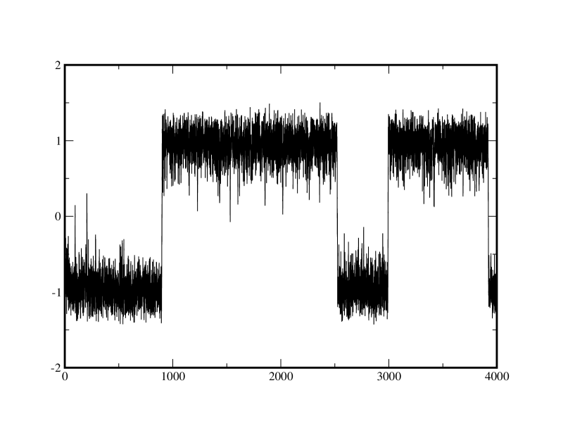
It follows that for most of the trajectory, the system makes uninteresting stochastic oscillations in the well, and can be described by normal mode analysis. Rarely, there is a very short but interesting physical phenomenon, which is the fast transition from one minimum to the other.

This picture has been confirmed by single molecule experiments 3 ; 4 , where the waiting time in one state can be measured, but the time for crossing from one state to the other is so short that it cannot be resolved. This scenario has also been confirmed recently by very long millisecond molecular dynamics simulations 14 which for the first time show spontaneous thermal folding-unfolding events.

According to Kramers theory, the total transition time $\tau_{K}$ (waiting + crossing) scales like the exponential of the barrier energy

$$\tau_{K}\sim e^{\Delta E/k_{B}T}$$

The “Kramers time” $\tau_{K}$ is the sum of two times:

• the waiting time in the potential well

• the crossing time over the barrier $\tau_{C}$

It is well known that the crossing time $\tau_{C}$ is small compared to $\tau_{K}$ and indeed, Hummer 15 and subsequently Szabo 16 have shown that

$$\tau_{C}\sim\ln\frac{\Delta E}{k_{B}T}<<\tau_{K}$$

These Kramers and crossing times are averages. In fact, these times are distributed (random variables) and single molecule experiments or long molecular dynamics simulations allow to compute their probability distributions.

However, it seems a bit wasteful to simulate proteins over huge time scales (milliseconds), during which only small conformational vibrations occur, just to observe interesting physical crossing events which occur very rarely, on the sub-microsecond scale.

The goal of this paper is to show how one can generate a representative sample of transition paths, starting in state A at time $0$ and ending in state B at some arbitrary time $t_{f}$. The typical times of interest are not the (long) folding times, but rather the (very short) transition or barrier crossing times. In mathematical terms, we are looking for the paths starting from A at time $0$ and conditioned to end in state B at time $t_{f}<<\tau_{K}$.

II The conditional probability

Using the path integral representation of eq.(9), we see that the probability for a path $\{x(t)\}$ starting at $x_{0}$ at time $0$, to end at $x_{f}$ at $t_{f}$ is given by

$$P(\{x(t)\})=\frac{1}{A}e^{-\beta(U(x_{f})-U(x_{0}))/2}\exp\left(-\frac{1}{4k_{B}T}\int_{0}^{t_{f}}dt\left(\gamma\dot{x^{2}}+\frac{1}{\gamma}V(x)\right)\right)$$ (10)

where

$$A=\int dx_{f}e^{-\beta(U(x_{f})-U(x_{0}))/2}\int_{(x_{0},0)}^{(x_{f},t_{f})}\mathcal{D}x(t)\exp\left(-\frac{1}{4k_{B}T}\int_{0}^{t_{f}}dt\left(\gamma\dot{x^{2}}+\frac{1}{\gamma}V(x)\right)\right)$$ (11)

The conditional probability over all paths starting at $x_{0}$ at time $0$ and ending at $x_{f}$ at time $t_{f}$, to find the system at point $x$ at an intermediate time $t$ is given by

$$\mathcal{P}(x,t)=\frac{1}{P(x_{f},t_{f}|x_{0},0)}Q(x,t)P(x,t)$$

where

$$P(x,t)=P(x,t|x_{0},0)$$

$$Q(x,t)=P(x_{f},t_{f}|x,t)$$

The equation satisfied by $P$ is given by (4), whereas that for $Q$ is given by

$$\frac{\partial Q}{\partial t}=-D\frac{\partial^{2}Q}{\partial x^{2}}+D\beta\frac{\partial U}{\partial x}\frac{\partial Q}{\partial x}$$ (12)

It follows easily that the equation for the conditional probability $\mathcal{P}(x,t)$ is given by

$$\frac{\partial\mathcal{P}}{\partial t}=D\frac{\partial}{\partial x}\left(\frac{\partial\mathcal{P}}{\partial x}+\frac{\partial}{\partial x}\left(\beta U-2\ln Q\right)\mathcal{P}\right)$$

Comparing this equation with the initial Fokker-Planck (4) and Langevin (1) equations, one sees that it can be obtained from a Langevin equation with a modified potential

$$\frac{dx}{dt}=-\frac{D}{k_{B}T}\frac{\partial U}{\partial x}+2D\frac{\partial\ln Q}{\partial x}+\eta(t)$$ (13)

This equation has been previously obtained using the Doob transform 17 and is known in the probability literature as a Langevin bridge: the paths $\{x(t)\}$ generated by (13) are conditioned to end at $(x_{f},t_{f}).$ It is the new term in the Langevin equation that guarantees that the trajectory starting at $(x_{0},0)$ will end at $(x_{f},t_{f}).$

Using eq.(7) for $Q$, one can write equation (13) as

$$\frac{dx}{dt}=2\frac{k_{B}T}{\gamma}\frac{\partial}{\partial x}\ln<x_{f}|e^{-(t_{f}-t)H}|x>+\eta(t)$$ (14)

Using the analogous of the correspondence principle of quantum mechanics 18 , i.e. $\frac{\hbar}{i}\frac{\partial}{\partial x}\rightarrow p$, this equation can also be rewritten in the form

$$\frac{dx}{dt}=<\dot{x}(t)>+\eta(t)$$ (15)

where by definition

$$<\dot{x}>=\frac{1}{<x_{f}|e^{-(t_{f}-t)H}|x>}\int_{(x,t)}^{(x_{f},t_{f})}\mathcal{D}x(\tau){\dot{x}(t)}\exp\left(-\frac{1}{4k_{B}T}\int_{t}^{t_{f}}d\tau\left(\gamma\dot{x^{2}}+\frac{1}{\gamma}V(x)\right)\right)$$ (16)

Note that for large time $t_{f}$, the matrix element in eq.(14) is dominated by the ground state of $H$, namely $<x_{f}|e^{-(t_{f}-t)H}|x>\sim e^{-\frac{\beta}{2}(U(x_{f})+U(x))}$ and as expected one recovers the standard (unconditioned) Langevin equation.

Since we have a natural splitting of the Hamiltonian $H$ as $H=H_{0}+V_{1}$ with $H_{0}=-\frac{k_{B}T}{\gamma}\frac{\partial^{2}}{\partial x^{2}}$ and $V_{1}=V/4\gamma k_{B}T$, it is convenient to rewrite the above equation as

$$\frac{dx}{dt}=2\frac{k_{B}T}{\gamma}\frac{\partial}{\partial x}\ln<x_{f}|e^{-(t_{f}-t)H_{0}}|x>+2\frac{k_{B}T}{\gamma}\frac{\partial}{\partial x}\ln\frac{<x_{f}|e^{-(t_{f}-t)H}|x>}{<x_{f}|e^{-(t_{f}-t)H_{0}}|x>}+\eta(t)$$ (17)

Note that the first term in the r.h.s. above is singular at $t=t_{f}$ and is thus responsible for driving the system to $(x_{f},t_{f})$ whereas the second one is regular. It follows that the first term is the only term which can drive the system to $(x_{f},t_{f})$, and any approximation which keeps the second term finite for $t=t_{f}$ will not affect this property.

This nice bridge equation cannot be used "as is", since we don’t know how to compute the function $Q$ or equivalently the matrix element in the above equation. There are many ways to approximate this function. It is important however, to preserve detailed balance as well as possible, that the approximation retains the symmetry of the matrix element.

III The modified Langevin equation and reweighting

The only approximation we found which remains local in time, i.e. which does not give rise to an integro-differential stochastic equation is the symmetric form of the Trotter approximation, commonly used in quantum mechanics 12 . Indeed, for short times $t$, a very simple and convenient symmetric approximation for $Q$ is given by

$$e^{-Ht}\sim e^{-tV_{1}/2}e^{-tH_{0}}e^{-tV_{1}/2}+O(t^{3})$$ (18)

which translates into

$$<x_{f}|e^{-Ht}|x>\sim e^{-\frac{\beta\gamma}{4t}(x_{f}-x)^{2}-\frac{\beta t}{8\gamma}(V(x_{f})+V(x))}$$

It would be nice to relate the range of validity of this equation to the spectrum of $H$. Indeed, as was shown before, the spectrum of $H$ corresponds to all the dynamical times of the system (folding times, transition times, etc…). We have not succeeded in finding such a relation except in the solvable case of the harmonic oscillator. In that case, it can easily be shawn that the natural expansion parameter is $t\Delta$ where $\Delta$ is the constant gap between the energy levels of $H$. As mentioned before, in the case of protein folding, the folding time which is the inverse of the first gap of the system can be very long, and we might expect the above approximation to be valid for times much smaller than this time. In particular, this approximation would allow to investigate the crossing times, much shorter than the folding time.

Plugging eq.(18) in eq.(26) we obtain the approximate Langevin bridge equation which in arbitrary dimension (or with arbitrary number of degrees of freedom) reads

$$\frac{d\vec{x}}{dt}=\frac{\vec{x}_{f}-\vec{x}}{t_{f}-t}-\frac{1}{4\gamma^{2}}(t_{f}-t)\nabla V(\vec{x})+\vec{\eta}(t)$$ (19)

where $\vec{\eta}(t)$ is a white noise vector whose components satisfy the relations (2) and (3) and

$$V(\vec{x})=\left(\nabla U\right)^{2}-2k_{B}T\nabla^{2}U$$ (20)

The first term in the r.h.s of eq.(19) is the one which drives the particle to reach $x_{f}$ at time $t_{f}$. The potential which governs this bridge equation is not the original $U(x)$ but rather the effective potential $V(x)$. Note also that the force term is proportional to $(t_{f}-t)$ and thus becomes small as the particle gets close to its target site.

In order to build a representative sample of paths starting at $(x_{0},0)$ and ending at $(x_{f},t_{f}),$ one must simply solve this equation for many different realizations of the random noise. Only the initial boundary condition is to be imposed, as the singular term in the equation imposes the correct final boundary condition. An important point to note is that all the trajectories generated by eq.(19) are statistically independent. From a numerical point of view, this means that this equation can be fully parallelized, and from a statistical point of view, it implies that all trajectories can be used in the representative sample. This last important point is to be contrasted with most existing methods where the sample are generated by some stochastic (Monte Carlo) methods which generate highly correlated trajectories.

Before presenting examples of application of this method, let us discuss how to correct for the fact that the total time $t_{f}$ should be small for the approximation to be valid.

Due to this restriction, the statistic of trajectories is not exact for larger times. Indeed, if eq.(19) were exact, each trajectory would be generated with its correct weight, and if one wanted to calculate observables, one would just have to compute simple white averages over all trajectories. However, as the equation is approximate, one needs to resample the ensemble of trajectories, that is, assign them a new weight. As we will show, the resampling weight is easily obtained.

Indeed, if we consider the sample of trajectories generated using eq.(19) between $(x_{0},0)$ and $(x_{f},t_{f})$, the weight of each trajectory should be given by eq.(10). However, it is clear from eq.(19) that, using the Ito prescription, the weight with which it was generated is given by

$$\exp\left(-\frac{\gamma}{4k_{B}T}\int_{0}^{t_{f}}dt\left(\frac{d\vec{x}}{dt}-\frac{\vec{x}_{f}-\vec{x}}{t_{f}-t}+\frac{t_{f}-t}{4\gamma^{2}}\nabla V(\vec{x})\right)^{2}\right)$$ (21)

Up to a normalization, the reweighting factor for a trajectory is thus given by

$$\exp\left(-\frac{\gamma}{4k_{B}T}\int_{0}^{t_{f}}dt\left(\left(\frac{d\vec{x}}{dt}+\frac{1}{\gamma}\nabla U\right)^{2}-\left(\frac{d\vec{x}}{dt}-\frac{\vec{x}_{f}-\vec{x}}{t_{f}-t}+\frac{t_{f}-t}{4\gamma^{2}}\nabla V(\vec{x})\right)^{2}\right)\right)$$ (22)

This quantity is easily calculated and allows for a correct evaluation of averages over paths.

This reweighting technique can also be used to generate paths statistically exactly sampled according to eq.(13). Indeed, consider eq.(15). The expectation value $<\dot{x}(t)>$ can be computed by generating at each time $t$ an ensemble of (approximate) trajectories starting from the current point $x$ at time $t$ and ending at $x_{f}$ at time $t_{f}$ by using eq.(19). By reweighting them using the weights of eq.(22), we can reliably compute $<\dot{x}(t)>$ and thus solve eq.(15). Note that this procedure which generates correctly weighted trajectories might seem computationally costly. However, since all trajectories are independent, they can efficiently be generated using massive parallelization.

IV The native state

Eq.(18) is in fact not quite valid between non normalizable states like $|x>$ and $|x_{f}>$, in that it is not true to order $O(t^{3})$. However it is true between a normalizable state and $|x>$. Assume that the final state of the system is defined by a probability distribution $\phi(x)$. For instance, for the case of a protein, $\phi(x)$ could represent the Boltzmann weight around the native state of the protein. The probability for the system to start at $x$ at time $t$ and end at time $t_{f}$ in the native state is given by

$$Q(x,t)=\int dy\ \phi(y)P(y,t_{f}|x,t)$$ (23)

or using (7)

$$Q(x,t)=\int dy\ \phi(y)e^{-\beta(U(y)-U(x))/2}<y|e^{-(t_{f}-t)H}|x>$$ (24)

where $\phi$ restricts the integration over $y$ to the vicinity of the native state.

With this definition of $Q$, it is straightforward to see that eq.(12) and (13) are still valid.

Using the approximation (18) we can write

$$Q(x,t)=e^{\beta U(x)/2}e^{-\frac{t}{2}V_{1}(x)}\int\frac{dy}{A}\ \phi(y)e^{-\beta U(y)/2}e^{-\frac{t}{2}V_{1}(y)}e^{-\frac{\beta\gamma}{4}\frac{(y-x)^{2}}{t_{f}-t}}$$ (25)

where $A=\sqrt{4\pi(t_{f}-t)/\beta\gamma}$.

As the function $\phi$ restricts the integration in (25) to the vicinity of the native state, we can approximate the potential $U(x)$ in this region by a quadratic expansion in terms of the normal modes

$$U(x)\simeq\frac{\omega}{2}(x-x_{f})^{2}$$

It follows that $V$ and $V_{1}$ are also quadratic and thus the integral (25) can be performed. Although we will consider only one-dimensional cases in the examples, we present the results for the multi-dimensional case.

Denoting by $\omega_{ij}=\frac{\partial^{2}U}{\partial x_{i}\partial x_{j}}|_{x_{i}^{f}}$ the Hessian matrix of normal modes around the native state, the potential $U$ can be written in that region as

$$U(x)=\frac{1}{2}\sum_{i,j}(x_{i}-x_{i}^{f})\omega_{ij}(x_{j}-x_{j}^{f})$$

and thus

$$V(x)=\sum_{i,j}(x_{i}-x_{i}^{f})\Omega_{ij}(x_{j}-x_{j}^{f})-2k_{B}T{\rm\,Tr}\ \omega_{ij}$$

where the symbol Tr denotes the trace of the normal mode matrix and

$$\Omega_{ij}=\sum_{k}\omega_{ik}\omega_{kj}$$

The function $Q$ can be easily calculated as

$$Q(x,t)=e^{-\frac{\beta}{8\gamma}(t_{f}-t)V(x)-\frac{\beta}{4}\sum_{i,j}(x_{I}^{f}-x_{i})W_{ij}(x_{j}^{f}-x_{j})}$$

where

$$W_{ij}=\sum_{k}D_{ik}(I+\frac{t_{f}-t}{\gamma}D)_{kj}^{-1}$$

where $I$ is the unit matrix and

$$D_{ij}=\omega_{ij}+\frac{t_{f}-t}{2\gamma}\Omega_{ij}$$

The bridge equation becomes then

$$\frac{dx_{i}}{dt}=\frac{1}{\gamma}\sum_{j}W_{ij}(x_{j}^{f}-x_{j})-\frac{1}{4\gamma^{2}}(t_{f}-t)\nabla_{i}V(\vec{x})+\eta_{i}(t)$$ (26)

V Including the solvent

In many cases, in particular protein folding, one wants to include explicitly the solvent molecules, most often water. It is thus desirable to generate trajectories which are conditioned for the protein coordinates, but not for the water molecules.

Denoting by $X_{i}$ the set of coordinates of the water molecules, the conditional probability, over all paths starting at $\{x_{0},X_{0}\}$ at time 0 and ending at $x_{f}$ at time $t_{f}$ (irrespective of the position of the solvent molecules), for the system to be at $\{x,X\}$ at time $t$ is given by

$$\mathcal{P}(x,X,t)=\frac{1}{\int dX_{f}P(x_{f},X_{f},t_{f}|x_{0},X_{0},0)}Q(x,X,t)P(x,X,t)$$

where

$$P(x,X,t) = P(x,X,t|x_{0},X_{0},0)$$ (27)

$$Q(x,X,t) = \int dX_{f}P(x_{f},X_{f},t_{f}|x,X,t)$$ (28)

The coordinates $X_{f}$ of the solvent are integrated over since the trajectories are not conditioned over the solvent molecules.

Using the method described in the previous sections, the exact generalized Langevin equations satisfied by the coordinates are

$$\frac{dx_{i}}{dt} = -\frac{D_{1}}{k_{B}T}\frac{\partial U}{\partial x_{i}}+2D_{1}\frac{\partial\ln Q}{\partial x_{i}}+\eta^{(1)}_{i}(t)$$ (29)

$$\frac{dX_{i}}{dt} = -\frac{D_{2}}{k_{B}T}\frac{\partial U}{\partial X_{i}}+2D_{2}\frac{\partial\ln Q}{\partial X_{i}}+\eta^{(2)}_{i}(t)$$ (30)

where $D_{1}$ and $D_{2}$ are resp. the diffusion constants for protein and water molecules and the Gaussian noises $\eta^{(1,2)}_{i}(t)$ satisfy the relation

$$<\eta^{(1,2)}_{i}(t)\ \eta^{(1,2)}_{j}(t^{\prime})>=2D_{1,2}\delta_{ij}\delta(t-t^{\prime})$$ (31)

Consider eq.(28). Let us show that the additional force term vanishes. Indeed,

$$Q(x,X,t) = \int dX_{f}P(x_{f},X_{f},t_{f}|x,X,t)$$ (32)

$$= \int dX_{f}P(x_{f}-x,X_{f}-X,t_{f}-t)$$

because of space and time translation invariance. Due to the integration over $X_{f}$ in eq.(32), we see that $Q(x,X,t)$ does not depend on $X$, and thus the new drift term in (30) is absent. Therefore the exact equations for the conditional probability in presence of solvent are

$$\frac{dx_{i}}{dt} = -\frac{D_{1}}{k_{B}T}\frac{\partial U}{\partial x_{i}}+2D_{1}\frac{\partial\ln Q}{\partial x_{i}}+\eta^{(1)}_{i}(t)$$ (33)

$$\frac{dX_{i}}{dt} = -\frac{D_{2}}{k_{B}T}\frac{\partial U}{\partial X_{i}}+\eta^{(2)}_{i}(t)$$ (34)

Using the Trotter approximation (18), these equations become (using vector notations)

$$\frac{d\vec{x}}{dt} = \frac{\vec{x}_{f}-\vec{x}}{t_{f}-t}-\frac{1}{4\gamma^{2}}(t_{f}-t)\nabla_{x}V(\vec{x},\vec{X})+\vec{\eta^{(1)}}(t)$$ (35)

$$\frac{d\vec{X}}{dt} = -\frac{D_{2}}{k_{B}T}\frac{\partial U(\vec{x},\vec{X})}{\partial\vec{X}}+\vec{\eta^{(2)}}(t)$$ (36)

where the noises are Gaussian, correlated according to eq.(31).

We thus conclude that in presence of the solvent, the protein is evolved through a modified Langevin equation with the effective potential $V(\vec{x},\vec{X})$, whereas the solvent molecules are evolved according to the standard Langevin equation in presence of the original potential $U(\vec{x},\vec{X})$.

Extension of this method to the case of the native state (see previous section) is immediate.

VI Example: The quartic double-well

We now illustrate the method on the example of barrier crossing in 1d (quartic potential).

$$U(x)=\frac{1}{4}(x^{2}-1)^{2}$$

This potential has two minima at $x=\pm 1$, separated by a barrier of height 1/4. Note that at low enough temperature, the potential $V(x)$ has two minima at points close to $\pm 1$ and one minimum at $x=0$ (from eq.(2)). Note that $V(x)$ is much steeper than $U(x)$ and thus more confining, around its minima.

Figure 2: Potential $U(x)$ (in black) and potential $V(x)$ (in red).

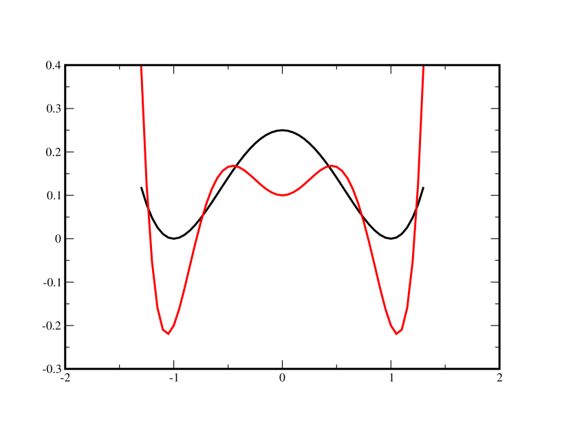
The model can be solved exactly by solving numerically the Fokker-Planck equation or by diagonalizing the Hamiltonian. All the examples are performed at low temperature $T=0.05$, where the barrier height is equal to 5 in units of $k_{B}T$ and the Kramers relaxation time, given by the inverse of the smallest non-zero eigenvalue of $H$, is equal to $\tau_{K}=366.39$.

On fig.3, we present a long trajectory ($t_{f}=1000)$ obtained by solving the Langevin eq.(1) for a particle starting at $x_{0}=-1$ at time 0. The general pattern described in the introduction can be easily checked: the particle stays in the left well for a time of the order of 550, then jumps very rapidly into the right well, where it stays for a time of the order of 200, then jumps back to the left well where it stays again a time equal to about 250.

Figure 3: Full Langevin trajectory during time $t_{f}=1000$ with 2 transitions between the minima

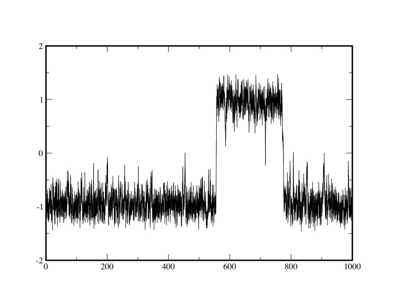
The two crossings times are very short, and we display an enlargement of the first transition in fig.4.

Figure 4: Enlargement of the first transition region

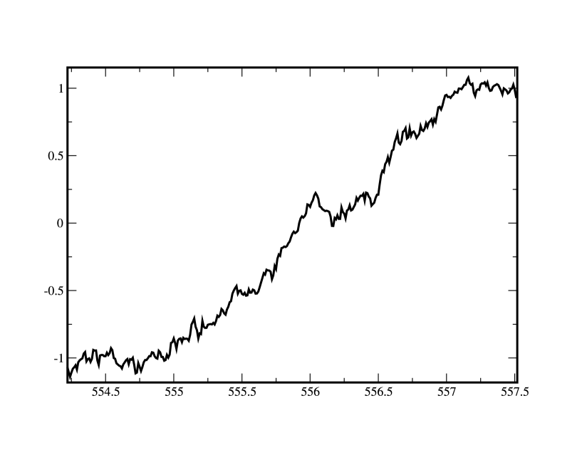
As can be seen, the crossing time for this specific trajectory is approximately $\tau_{C}\thickapprox 2.5$, much smaller than the Kramers time.

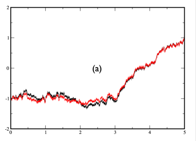
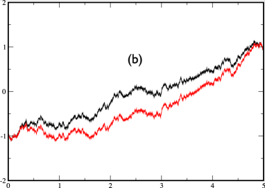
In fig.5, we plot two examples of two trajectories conditioned to cross the barrier during a time $t_{f}=5.$ The trajectory in black is obtained by solving the exact bridge eq.(14) by computing exactly (using a spectral decomposition) the matrix element of the evolution operator, while the trajectory in red is obtained by solving the approximate eq.(19) with the exact same sequence of noise $\eta(t)$. In the left figure, the 2 trajectories are barely distinguishable, whereas the agreement is not as spectacular on the right figure.

Figure 5: Two sets (a) and (b) of exact trajectories (in black) and approximate trajectories (in red)

Next we look at some observables, obtained by averaging over many trajectories.

In fig.6, we plot: in black the exact average $x(t)$ (obtained by a full expansion over the eigenstates of $H$), in red the average $x(t)$ over 2000 trajectories obtained by solving eq.(19), and in blue, the average $x(t)$ obtained by reweighting the trajectories according to eq.(22) . Plot (a) is obtained for $t_{f}=2$, plot (b) for $t_{f}=5$ and plot (c) for $t_{f}=10$.

Figure 6: Average position as a function of time for (a) $t_{f}=2$, (b) $t_{f}=5$, (c) $t_{f}=10$. Black curve: exact. Red curve: approximate. Blue curve: reweighted

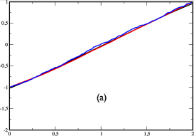
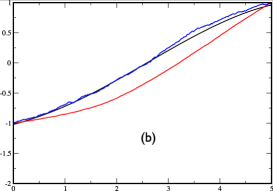
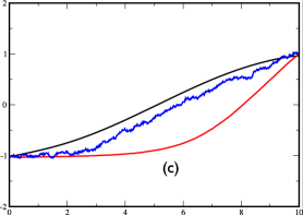
As expected, we see that the discrepancy between the exact (black) and the approximate (red) average $x(t)$ increases with $t_{f}$. For times shorter than the transition time $\tau_{C}$, the agreement is excellent, whereas for $t_{f}=10>\tau_{C}$, the agreement is not as good. However, we see that the reweighting procedure, although not perfect, improves drastically the quality of the average for large $t_{f}$.

One of the main defects which appears in the approximate theory is the following: In the exact theory, the transition between the 2 minima can take place at any time between 0 and $t_{f}$. By contrast, it seems that in the approximate theory, the transition is driven by the final state and takes place only in the end of the trajectory. This effect remains negligible as long as $t_{f}\lesssim\tau_{C}$ but becomes important for $t_{f}>$$\tau_{c}$. We illustrate this problem in fig.7 for $t_{f}=10$. On the left figure, the exact and approximate trajectories make their transition in the last part of the time, whereas in the right figure, the real trajectory crosses in the beginning while the approximate trajectory still crosses in the last part.

Figure 7: Two sets (a) and (b) of trajectories conditioned to cross the barrier. In black, exact trajectories and in red, approximate trajectories.

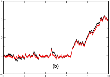
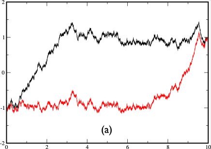
However, as we are interested quantitatively only in the region where the particle crosses the barrier, one can make long runs of approximate trajectories: They will not be good approximations of the real trajectories, except in the end of the trajectory where the transition to the final state occurs.

VII Conclusion

We have presented in this paper a novel method to generate paths following the Langevin overdamped dynamics, starting from an initial configuration and conditioned to end in a given final configuration (point or region of configuration space). We propose an approximation which is valid for small times. We have not been able to quantify how small should the time be, but the approximate dynamics seems to correctly reproduce the transition through a barrier. The approximate dynamics seems to have a tendency to confine the system in its initial configuration, and to allow for the transition only in the final stages. But this is not really a drawback since if we evolve approximately the system over long times, it will remain close to its initial condition, thus generating unreliable trajectories. However in the latest stages, the system will make its transition to the final state during a short time for which our approximation is reliable.

One of the great advantages of this method is that all generated trajectories are statistically independent. It is thus very easy to generate many of these trajectories using parallel computers. In addition, the trajectories can be reweighted to provide a faithful sample of the exact stochastic dynamics. Finally, this reweighting technique allows for the calculation of the matrix element of the evolution operator, and thus allows for the generation of adequately sampled paths.

The paths generated by our method can also be used either as initial paths to perform Monte Carlo transition path sampling, or as initial conditions for path minimization to determine Dominant Folding Paths.

The method is as simple to implement as ordinary Langevin dynamics, and its application to simple models of protein folding is currently under way.