Triviality and vacuum stability bounds in the three-loop
neutrino mass model

Mayumi Aoki mayumi@hep.s.kanazawa-u.ac.jp Institute for Theoretical Physics, Kanazawa University, Kanazawa 920-1192,  Japan    Shinya Kanemura kanemu@sci.u-toyama.ac.jp Department of Physics, University of Toyama, 3190 Gofuku, Toyama 930-8555, Japan    Kei Yagyu keiyagyu@jodo.sci.u-toyama.ac.jp Department of Physics, University of Toyama, 3190 Gofuku, Toyama 930-8555, Japan
Abstract

We study theoretical constraints on the parameter space under the conditions from vacuum stability and triviality in the three-loop radiative seesaw model with TeV-scale right-handed neutrinos which are odd under the Z2subscript𝑍2Z_{2} parity. In this model, some of the neutrino Yukawa coupling constants can be of the order of one. Requirement of strongly first order phase transition for successful electroweak baryogenesis also prefers order-one coupling constants in the scalar sector. Hence, it is important to clarify whether this model satisfies those theoretical conditions up to a given cutoff scale. It is found that the model can be consistent up to the scale above 10 TeV in the parameter region where the neutrino data, the lepton flavor violation data, the thermal relic abundance of dark matter as well as the requirement from the strongly first order phase transition are satisfied.

pacs:
preprint: KANAZAWA-11-01, UT-HET 035

I Introduction

The Higgs sector is the last unknown part in the standard model (SM). There is no compelling reason that it takes its minimal form. Instead, there can be various possibilities for non-minimal Higgs sectors. Currently, searches for the Higgs boson is underway at the Tevatron and the Large Hadron Collider (LHC). It is expected that crucial information for the Higgs sector will be obtained in near future. On the other hand, there are phenomena which cannot explain within the SM such as neutrino oscillation, existence of dark matter, and baryon asymmetry of the Universe. They provide us strong motivations to consider physics beyond the SM.

The Higgs sector may be related to the physics to cause these phenomena. First of all, based on the WIMP (Weakly Interacting Massive Particle) hypothesis, the observed value of the relic abundance requires the mass of the dark matter to be around the electroweak scale. Why is the mass of the WIMP dark matter at the electroweak scale? This would strongly indicate a direct connection between the WIMP dark matter and the Higgs sector Bento:2000ah ; higgsportal . Second, the origin of neutrino masses may also be the TeV scale: i.e., the origin of the lepton number violation would be the existence of TeV-scale right-handed neutrinos or that of lepton number violating scalar interactions in the extended Higgs sector. As a natural scenario for generating tiny neutrino masses, such lepton number violation at the TeV scale would be transmitted to the left-handed neutrino sector via loop effects of the Higgs sectors. This is so-called the radiative seesaw scenario zee ; zeebabu ; knt ; ma ; aks-prl . Finally, a simple description of baryon asymmetry of the Universe may be the scenario in which electroweak phase transition is of strongly first order in order to satisfy the Sakharov’s condition of departure from thermal equilibrium sakharov . This is the scenario of electroweak baryogenesis ewbg .

An attractive point for these scenarios would be that they can give definite predictions to TeV-scale phenomenology, so that we can directly test them by experiments, in principle. Various scenarios for the WIMP dark matter can be tested by direct and indirect searches as well as collider experiments Bento:2000ah ; higgsportal ; Ma-DM . Each radiative seesaw model predicts a characteristic extended Higgs sector with lepton number violating interactions zee ; kkloy ; zeebabu ; babu-macesanu ; szb or right-handed neutrinos knt ; kingman-seto ; ma ; radiative ; CaoMa . It is known that the dynamics for the electroweak baryogenesis strongly related to the Higgs boson phenomenology at colliders ewbg-thdm2 .

Therefore, an interesting question is whether or not we can construct a successful TeV-scale phenomenological model where these three phenomena would be explained simultaneously. Recently a TeV-scale model has been proposed for such a purpose aks-prl , in which 1) tiny neutrino masses are generated without excessive fine tuning at the three-loop level by the dynamics of an extended Higgs sector and right-handed neutrinos under an unbroken Z2subscript𝑍2Z_{2} parity, 2) the Z2subscript𝑍2Z_{2} parity also guaranties the stability of a dark matter candidate which is a Z2subscript𝑍2Z_{2} odd scalar boson, and 3) the strongly first order phase transition for successful electroweak baryogenesis can be realized by the non-decoupling effect in the Higgs sector. Phenomenology of this model has been discussed in Ref. aks-prd , and the related collider physics typeX ; stefano ; ak-majorana and dark matter properties aks-cdms2 have also been studied. In these papers, phenomenologically allowed parameter regions have been mainly discussed.

In this paper, we investigate the theoretical constraint on the parameter regions in this model aks-prl from the requirement of vacuum stability and perturbativity up to a given cutoff scale ΛΛ\Lambda of the model cabibbo . In the present model, there is no mechanism for cancellation of the quadratic divergences which appear in the renormalization calculation for the Higgs boson mass, so that a huge fine tuning is required if ΛΛ\Lambda is much higher than the electroweak scale. To avoid such an unnatural situation, we need to consider ΛΛ\Lambda to be at most 𝒪(10)𝒪10{\cal O}(10) TeV, above which the model would be replaced by a more fundamental theory Murayama . Hence, we have to study the theoretical consistency of the model up to such values for ΛΛ\Lambda. In particular, some of the neutrino Yukawa coupling constants are of order one in magnitude, as the scale of tiny neutrino masses is generated by loop dynamics so that we do not need fine tuning for the size of the coupling constants. In addition, some of the coupling constants in the Higgs potential are of order one to realize the non-decoupling one-loop effect for strongly first order phase transition. Although the parameters discussed in the previous works satisfy the bound from tree-level unitarity pu_nonminimum , it is non-trivial that the model can be consistent at the quantum level with the theoretical requirements up to Λ10similar-toΛ10\Lambda\sim 10 TeV. Theoretical bounds from vacuum stability and perturbativity have been used to constrain parameters in extended Higgs sectors such as the two Higgs doublet model vs_thdm and the Zee model kkloy . Here we apply the similar analysis to the model. We prepare a full set of the renormalization group equations (RGEs) for dimensionless coupling constants in the model at the one-loop level, and analyze the behavior of running coupling constants.

We also revise the phenomenological constraint from lepton flavor violation (LFV) in the model. In the previous analysis aks-prl ; aks-prd only the constraint from μeγ𝜇𝑒𝛾\mu\rightarrow e\gamma data has been taken into account. Here, we also analyze the one-loop induced μeee𝜇𝑒𝑒𝑒\mu\rightarrow eee process, whose current experimental data meee turn out to give a stronger bound on the parameter space than those of μeγ𝜇𝑒𝛾\mu\rightarrow e\gamma MEGA 111 We thank Toru Goto for telling us the possibility of a sizable contribution to the branching ratio of μeee𝜇𝑒𝑒𝑒\mu\rightarrow eee in our model..

The paper is organized as follows. In Sec.II, we give a brief review of the model. In Sec.III, we introduce the criteria for vacuum stability and triviality, and numerical results of the RGE analysis are presented. In Sec.IV, we give a conclusion.

II The three-loop neutrino mass model

We give a short review for the the three-loop neutrino mass model in Ref. aks-prl to make the paper self-contained.

II.1 Model

In this model, two Higgs doublets (Φ1subscriptΦ1\Phi_{1} and Φ2subscriptΦ2\Phi_{2}) with hypercharge Y=1/2𝑌12Y=1/2, charged scalar singlets (S±superscript𝑆plus-or-minusS^{\pm}), a real scalar singlet (η𝜂\eta) and right-handed neutrinos (NRαsuperscriptsubscript𝑁𝑅𝛼N_{R}^{\alpha} with α=1,2𝛼12\alpha=1,2) are introduced. We impose two kinds of discrete symmetries; i.e., Z2subscript𝑍2Z_{2} and Z~2subscript~𝑍2\tilde{Z}_{2} to the model. The former, which is exact, is introduced in order to forbid the tree-level Dirac neutrino mass term and at the same time to guarantee the stability of dark matter. The latter one, which is softly broken, is introduced to avoid the tree-level flavor changing neutral current fcnc . Under the Z~2subscript~𝑍2\tilde{Z}_{2} symmetry there are four types of Yukawa interactions Ref:Barger ; grossman . In our model aks-prl , so-called the type-X Yukawa interaction typeX ; typeX2 is favored since the charged Higgs boson from the two doublets can be taken to be as light as around 100 GeV without contradicting the bsγ𝑏𝑠𝛾b\rightarrow s\gamma data. Such a light charged Higgs boson is important to reproduce the correct magnitude of neutrino masses. The particle properties under the discrete symmetries are shown in Table 1, where QLisuperscriptsubscript𝑄𝐿𝑖Q_{L}^{i}, uRisuperscriptsubscript𝑢𝑅𝑖u_{R}^{i}, dRisuperscriptsubscript𝑑𝑅𝑖d_{R}^{i}, LLisuperscriptsubscript𝐿𝐿𝑖L_{L}^{i} and eRisuperscriptsubscript𝑒𝑅𝑖e_{R}^{i} are the i𝑖i-th generation of the left-handed quark doublet, the right-handed up-type quark singlet, the left-handed lepton doublet and the right-handed charged lepton singlet, respectively.

QLiuRidRiLLieRisuperscriptsubscript𝑄𝐿𝑖superscriptsubscript𝑢𝑅𝑖superscriptsubscript𝑑𝑅𝑖superscriptsubscript𝐿𝐿𝑖superscriptsubscript𝑒𝑅𝑖Q_{L}^{i}\hskip 2.84526ptu_{R}^{i}\hskip 2.84526ptd_{R}^{i}\hskip 2.84526ptL_{L}^{i}\hskip 2.84526pte_{R}^{i} Φ1Φ2subscriptΦ1subscriptΦ2\Phi_{1}\hskip 2.84526pt\Phi_{2} S±ηNRαsuperscript𝑆plus-or-minus𝜂superscriptsubscript𝑁𝑅𝛼S^{\pm}\hskip 2.84526pt\eta\hskip 2.84526ptN_{R}^{\alpha}
Z2subscript𝑍2Z_{2}(exact) ++++++\hskip 5.69054pt+\hskip 5.69054pt+\hskip 5.69054pt+\hskip 5.69054pt+ +++\hskip 5.69054pt+ -\hskip 5.69054pt-\hskip 5.69054pt-
Z~2subscript~𝑍2\tilde{Z}_{2}(softly broken) ++++\hskip 5.69054pt-\hskip 5.69054pt-\hskip 5.69054pt+\hskip 5.69054pt+ ++\hskip 5.69054pt- +++\hskip 5.69054pt-\hskip 5.69054pt+
Table 1: Particle properties under the discrete symmetries.

The type-X Yukawa interaction is given by

yukawaType-XsuperscriptsubscriptyukawaType-X\displaystyle\mathcal{L}_{\text{yukawa}}^{\text{Type-X}} =i,j[(Q¯LiYijdΦ2dRj)+(Q¯LiYijuΦ2cuRj)+(L¯LiYijeΦ1eRj)]+h.c.,formulae-sequenceabsentsubscript𝑖𝑗delimited-[]superscriptsubscript¯𝑄𝐿𝑖subscriptsuperscript𝑌𝑑𝑖𝑗subscriptΦ2superscriptsubscript𝑑𝑅𝑗superscriptsubscript¯𝑄𝐿𝑖subscriptsuperscript𝑌𝑢𝑖𝑗subscriptsuperscriptΦ𝑐2superscriptsubscript𝑢𝑅𝑗superscriptsubscript¯𝐿𝐿𝑖subscriptsuperscript𝑌𝑒𝑖𝑗subscriptΦ1superscriptsubscript𝑒𝑅𝑗hc\displaystyle=-\sum_{i,j}\left[\left(\bar{Q}_{L}^{i}Y^{d}_{ij}\Phi_{2}d_{R}^{j}\right)+\left(\bar{Q}_{L}^{i}Y^{u}_{ij}\Phi^{c}_{2}u_{R}^{j}\right)+\left(\bar{L}_{L}^{i}Y^{e}_{ij}\Phi_{1}e_{R}^{j}\right)\right]+{\rm h.c.}, (1)

where Yukawa coupling matrix for leptons is diagonal, Yije=diag(ye1,ye2,ye3)subscriptsuperscript𝑌𝑒𝑖𝑗diagsubscript𝑦superscript𝑒1subscript𝑦superscript𝑒2subscript𝑦superscript𝑒3Y^{e}_{ij}={\rm diag}(y_{e^{1}},y_{e^{2}},y_{e^{3}}). The mass term and the Yukawa interaction for NRαsuperscriptsubscript𝑁𝑅𝛼N_{R}^{\alpha} are written as

NRsubscriptsubscript𝑁𝑅\displaystyle\mathcal{L}_{N_{R}} =α=1212mNRα(NRα)c¯NRαi=13α=12[hiα(eRi)c¯NRαS++h.c.].\displaystyle=\sum_{\alpha=1}^{2}\frac{1}{2}m_{N_{R}^{\alpha}}\overline{(N_{R}^{\alpha})^{c}}N_{R}^{\alpha}-\sum_{i=1}^{3}\sum_{\alpha=1}^{2}\left[h_{i}^{\alpha}\overline{(e_{R}^{i})^{c}}N_{R}^{\alpha}S^{+}+{\rm h.c.}\right]. (2)

The scalar potential is given by

V=𝑉absent\displaystyle V= +μ12|Φ1|2+μ22|Φ2|2[μ32Φ1Φ2+h.c.]\displaystyle+\mu_{1}^{2}|\Phi_{1}|^{2}+\mu_{2}^{2}|\Phi_{2}|^{2}-\Big{[}\mu_{3}^{2}\Phi_{1}^{\dagger}\Phi_{2}+{\rm h.c.}\Big{]}
+12λ1|Φ1|4+12λ2|Φ2|4+λ3|Φ1|2|Φ2|2+λ4|Φ1Φ2|2+12[λ5(Φ1Φ2)2+h.c.]\displaystyle+\frac{1}{2}\lambda_{1}|\Phi_{1}|^{4}+\frac{1}{2}\lambda_{2}|\Phi_{2}|^{4}+\lambda_{3}|\Phi_{1}|^{2}|\Phi_{2}|^{2}+\lambda_{4}|\Phi_{1}^{\dagger}\Phi_{2}|^{2}+\frac{1}{2}\Big{[}\lambda_{5}(\Phi_{1}^{\dagger}\Phi_{2})^{2}+{\rm h.c.}\Big{]}
+μS2|S|2+ρ1|S|2|Φ1|2+ρ2|S|2|Φ2|2+14λS|S|4superscriptsubscript𝜇𝑆2superscriptsuperscript𝑆2subscript𝜌1superscriptsuperscript𝑆2superscriptsubscriptΦ12subscript𝜌2superscriptsuperscript𝑆2superscriptsubscriptΦ2214subscript𝜆𝑆superscriptsuperscript𝑆4\displaystyle+\mu_{S}^{2}|S^{-}|^{2}+\rho_{1}|S^{-}|^{2}|\Phi_{1}|^{2}+\rho_{2}|S^{-}|^{2}|\Phi_{2}|^{2}+\frac{1}{4}\lambda_{S}|S^{-}|^{4}
+12μη2η2+12σ1η2|Φ1|2+12σ2η2|Φ2|2+14!ληη412superscriptsubscript𝜇𝜂2superscript𝜂212subscript𝜎1superscript𝜂2superscriptsubscriptΦ1212subscript𝜎2superscript𝜂2superscriptsubscriptΦ2214subscript𝜆𝜂superscript𝜂4\displaystyle+\frac{1}{2}\mu_{\eta}^{2}\eta^{2}+\frac{1}{2}\sigma_{1}\eta^{2}|\Phi_{1}|^{2}+\frac{1}{2}\sigma_{2}\eta^{2}|\Phi_{2}|^{2}+\frac{1}{4!}\lambda_{\eta}\eta^{4}
+a,b=12[κϵab(Φac)ΦbSη+h.c.]+12ξ|S|2η2,\displaystyle+\sum_{a,b=1}^{2}\Big{[}\kappa\epsilon_{ab}(\Phi_{a}^{c})^{\dagger}\Phi_{b}S^{-}\eta+{\rm h.c.}\Big{]}+\frac{1}{2}\xi|S^{-}|^{2}\eta^{2}, (3)

where ϵabsubscriptitalic-ϵ𝑎𝑏\epsilon_{ab} are anti-symmetric matrices with ϵ12=1subscriptitalic-ϵ121\epsilon_{12}=1. The parameters μ32superscriptsubscript𝜇32\mu_{3}^{2}, λ5subscript𝜆5\lambda_{5}, and κ𝜅\kappa are complex numbers. Two of their phases can be absorbed by rephasing the fields, and the rest is a physical one. In this paper, we neglect this CP-violating phase for simplicity. The Higgs doublets are parameterized as

Φi=(wi+12(hi+vi+izi)),subscriptΦ𝑖superscriptsubscript𝑤𝑖12subscript𝑖subscript𝑣𝑖𝑖subscript𝑧𝑖\displaystyle\Phi_{i}=\left(\begin{array}[]{c}w_{i}^{+}\\ \frac{1}{\sqrt{2}}(h_{i}+v_{i}+iz_{i})\end{array}\right), (6)

where visubscript𝑣𝑖v_{i} are vacuum expectation values (VEVs) of the Higgs fields, and these are constrained by v(=v12+v22)246similar-to-or-equalsannotated𝑣absentsuperscriptsubscript𝑣12superscriptsubscript𝑣22246v(=\sqrt{v_{1}^{2}+v_{2}^{2}})\simeq 246 GeV. The ratio of the two VEVs is defined by tanβ=v2/v1𝛽subscript𝑣2subscript𝑣1\tan\beta=v_{2}/v_{1}. The physical scalar states hh, H𝐻H, A𝐴A and H±superscript𝐻plus-or-minusH^{\pm} in the Z2subscript𝑍2Z_{2} even sector can be obtained mixing angles α𝛼\alpha and β𝛽\beta,

(w1±w2±)=R(β)(w±H±),(z1z2)=R(β)(zA),(h1h2)=R(α)(Hh),formulae-sequencesuperscriptsubscript𝑤1plus-or-minussuperscriptsubscript𝑤2plus-or-minus𝑅𝛽superscript𝑤plus-or-minussuperscript𝐻plus-or-minusformulae-sequencesubscript𝑧1subscript𝑧2𝑅𝛽𝑧𝐴subscript1subscript2𝑅𝛼𝐻\displaystyle\left(\begin{array}[]{c}w_{1}^{\pm}\\ w_{2}^{\pm}\end{array}\right)=R(\beta)\left(\begin{array}[]{c}w^{\pm}\\ H^{\pm}\end{array}\right),\hskip 8.53581pt\left(\begin{array}[]{c}z_{1}\\ z_{2}\end{array}\right)=R(\beta)\left(\begin{array}[]{c}z\\ A\end{array}\right),\hskip 8.53581pt\left(\begin{array}[]{c}h_{1}\\ h_{2}\end{array}\right)=R(\alpha)\left(\begin{array}[]{c}H\\ h\end{array}\right), (19)

where w±superscript𝑤plus-or-minusw^{\pm} and z𝑧z are the Nambu-Goldstone bosons absorbed by the longitudinal weak gauge bosons, and the rotation matrix with the angle θ𝜃\theta is given by

R(θ)=(cosθsinθsinθcosθ).𝑅𝜃𝜃𝜃𝜃𝜃\displaystyle R(\theta)=\left(\begin{array}[]{cc}\cos\theta&-\sin\theta\\ \sin\theta&\cos\theta\end{array}\right). (22)

The mass formulae of physical scalar states are given by

mA2superscriptsubscript𝑚𝐴2\displaystyle m_{A}^{2} =M2v2λ5,absentsuperscript𝑀2superscript𝑣2subscript𝜆5\displaystyle=M^{2}-v^{2}\lambda_{5}, (23)
mH±2superscriptsubscript𝑚superscript𝐻plus-or-minus2\displaystyle m_{H^{\pm}}^{2} =M2v22(λ4+λ5),absentsuperscript𝑀2superscript𝑣22subscript𝜆4subscript𝜆5\displaystyle=M^{2}-\frac{v^{2}}{2}(\lambda_{4}+\lambda_{5}), (24)
mH2superscriptsubscript𝑚𝐻2\displaystyle m_{H}^{2} =cos2(αβ)M112+2sin(αβ)cos(αβ)M122+sin2(αβ)M222,absentsuperscript2𝛼𝛽superscriptsubscript𝑀1122𝛼𝛽𝛼𝛽superscriptsubscript𝑀122superscript2𝛼𝛽superscriptsubscript𝑀222\displaystyle=\cos^{2}(\alpha-\beta)M_{11}^{2}+2\sin(\alpha-\beta)\cos(\alpha-\beta)M_{12}^{2}+\sin^{2}(\alpha-\beta)M_{22}^{2}, (25)
mh2superscriptsubscript𝑚2\displaystyle m_{h}^{2} =sin2(αβ)M1122sin(αβ)cos(αβ)M122+cos2(αβ)M222,absentsuperscript2𝛼𝛽superscriptsubscript𝑀1122𝛼𝛽𝛼𝛽superscriptsubscript𝑀122superscript2𝛼𝛽superscriptsubscript𝑀222\displaystyle=\sin^{2}(\alpha-\beta)M_{11}^{2}-2\sin(\alpha-\beta)\cos(\alpha-\beta)M_{12}^{2}+\cos^{2}(\alpha-\beta)M_{22}^{2}, (26)
mS2superscriptsubscript𝑚𝑆2\displaystyle m_{S}^{2} =μS2+v22ρ1cos2β+v22ρ2sin2β,absentsuperscriptsubscript𝜇𝑆2superscript𝑣22subscript𝜌1superscript2𝛽superscript𝑣22subscript𝜌2superscript2𝛽\displaystyle=\mu_{S}^{2}+\frac{v^{2}}{2}\rho_{1}\cos^{2}\beta+\frac{v^{2}}{2}\rho_{2}\sin^{2}\beta, (27)
mη2superscriptsubscript𝑚𝜂2\displaystyle m_{\eta}^{2} =μη2+v22σ1cos2β+v22σ2sin2β,absentsuperscriptsubscript𝜇𝜂2superscript𝑣22subscript𝜎1superscript2𝛽superscript𝑣22subscript𝜎2superscript2𝛽\displaystyle=\mu_{\eta}^{2}+\frac{v^{2}}{2}\sigma_{1}\cos^{2}\beta+\frac{v^{2}}{2}\sigma_{2}\sin^{2}\beta, (28)

where M(=μ3/sinβcosβ)annotated𝑀absentsubscript𝜇3𝛽𝛽M(=\mu_{3}/\sqrt{\sin\beta\cos\beta}) is the soft breaking scale for the Z~2subscript~𝑍2\tilde{Z}_{2} symmetry, and

M112superscriptsubscript𝑀112\displaystyle M_{11}^{2} =v2(λ1cos4β+λ2sin4β)+v22λsin22β,absentsuperscript𝑣2subscript𝜆1superscript4𝛽subscript𝜆2superscript4𝛽superscript𝑣22𝜆superscript22𝛽\displaystyle=v^{2}(\lambda_{1}\cos^{4}\beta+\lambda_{2}\sin^{4}\beta)+\frac{v^{2}}{2}\lambda\sin^{2}2\beta, (29)
M222superscriptsubscript𝑀222\displaystyle M_{22}^{2} =M2+v2sin2βcos2β(λ1+λ22λ),absentsuperscript𝑀2superscript𝑣2superscript2𝛽superscript2𝛽subscript𝜆1subscript𝜆22𝜆\displaystyle=M^{2}+v^{2}\sin^{2}\beta\cos^{2}\beta(\lambda_{1}+\lambda_{2}-2\lambda), (30)
M122superscriptsubscript𝑀122\displaystyle M_{12}^{2} =v2sinβcosβ(λ1cos2β+λ2sin2β+λcos2β),absentsuperscript𝑣2𝛽𝛽subscript𝜆1superscript2𝛽subscript𝜆2superscript2𝛽𝜆2𝛽\displaystyle=v^{2}\sin\beta\cos\beta(-\lambda_{1}\cos^{2}\beta+\lambda_{2}\sin^{2}\beta+\lambda\cos 2\beta), (31)

with λ=λ3+λ4+λ5𝜆subscript𝜆3subscript𝜆4subscript𝜆5\lambda=\lambda_{3}+\lambda_{4}+\lambda_{5}. Notice that M𝑀M, μSsubscript𝜇𝑆\mu_{S} and μηsubscript𝜇𝜂\mu_{\eta} are free mass parameters irrelevant to the electroweak symmetry breaking.

II.2 Neutrino mass and mixing
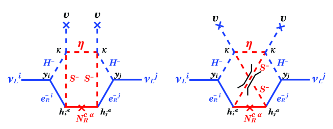
Refer to caption
Figure 1: The Feynman diagrams for generating tiny neutrino masses.

The neutrino mass matrix Mijνsubscriptsuperscript𝑀𝜈𝑖𝑗M^{\nu}_{ij} is generated by the three-loop diagrams in FIG. 1. The absence of lower order loop contributions is guaranteed by the Z2subscript𝑍2Z_{2} symmetry. The resulting mass matrix is calculated as

Mijνsubscriptsuperscript𝑀𝜈𝑖𝑗\displaystyle M^{\nu}_{ij} =\displaystyle= α=124κ2tan2β(yiSMhiα)(yjSMhjα)F(mH±,mS,mNRα,mη),superscriptsubscript𝛼124superscript𝜅2superscript2𝛽superscriptsubscript𝑦subscript𝑖SMsuperscriptsubscript𝑖𝛼superscriptsubscript𝑦subscript𝑗SMsuperscriptsubscript𝑗𝛼𝐹subscript𝑚superscript𝐻plus-or-minussubscript𝑚𝑆subscript𝑚superscriptsubscript𝑁𝑅𝛼subscript𝑚𝜂\displaystyle\sum_{\alpha=1}^{2}4\kappa^{2}\tan^{2}\beta(y_{\ell_{i}}^{\rm SM}h_{i}^{\alpha})(y_{\ell_{j}}^{\rm SM}h_{j}^{\alpha})F(m_{H^{\pm}},m_{S},m_{N_{R}^{\alpha}},m_{\eta}), (32)

where the loop integral function F𝐹F is given by

F(mH±,mS,mN,mη)=(116π2)3(mN)mN2mη2v2mH±4𝐹subscript𝑚superscript𝐻plus-or-minussubscript𝑚𝑆subscript𝑚𝑁subscript𝑚𝜂superscript116superscript𝜋23subscript𝑚𝑁superscriptsubscript𝑚𝑁2superscriptsubscript𝑚𝜂2superscript𝑣2superscriptsubscript𝑚superscript𝐻plus-or-minus4\displaystyle F(m_{H^{\pm}},m_{S},m_{N},m_{\eta})=\left(\frac{1}{16\pi^{2}}\right)^{3}\frac{(-m_{N})}{m_{N}^{2}-m_{\eta}^{2}}\frac{v^{2}}{m_{H^{\pm}}^{4}}
×0xdx{B1(x,mH±,mS)B1(x,0,mS)}2(mN2x+mN2mη2x+mη2),\displaystyle\times\int_{0}^{\infty}xdx\left\{B_{1}(-x,m_{H^{\pm}},m_{S})-B_{1}(-x,0,m_{S})\right\}^{2}\left(\frac{m_{N}^{2}}{x+m_{N}^{2}}-\frac{m_{\eta}^{2}}{x+m_{\eta}^{2}}\right), (33)

with yiSM=2mi/vsuperscriptsubscript𝑦subscript𝑖SM2subscript𝑚subscript𝑖𝑣y_{\ell_{i}}^{\rm SM}=\sqrt{2}m_{\ell_{i}}/v, where 1subscript1\ell_{1}, 2subscript2\ell_{2} and 3subscript3\ell_{3} correspond to e𝑒e, μ𝜇\mu and τ𝜏\tau, respectively. The function B1subscript𝐵1B_{1} is the tensor coefficient in the formalism by Passarino-Veltman for one-loop integrals passarino-veltman . In the following discussion, we take mNR1=mNR2mNRsubscript𝑚superscriptsubscript𝑁𝑅1subscript𝑚superscriptsubscript𝑁𝑅2subscript𝑚subscript𝑁𝑅m_{N_{R}^{1}}=m_{N_{R}^{2}}\equiv m_{N_{R}}, for simplicity. Numerically, the magnitude of the function F𝐹F is of order 104superscript10410^{4} eV in the wide range of parameter regions of our interest. Since yiSM<102superscriptsubscript𝑦subscript𝑖SMsuperscript102y_{\ell_{i}}^{\rm SM}<10^{-2}, the correct scale of neutrino masses can be naturally obtained from the three-loop diagrams.

The generated mass matrix Mijνsubscriptsuperscript𝑀𝜈𝑖𝑗M^{\nu}_{ij} in Eq. (32) of neutrinos can be related to the neutrino oscillation data by

Mijν=Uis(Mdiagν)st(UT)tj,subscriptsuperscript𝑀𝜈𝑖𝑗subscript𝑈𝑖𝑠subscriptsubscriptsuperscript𝑀𝜈diag𝑠𝑡subscriptsuperscript𝑈𝑇𝑡𝑗\displaystyle M^{\nu}_{ij}=U_{is}(M^{\nu}_{\rm diag})_{st}(U^{T})_{tj}, (34)

where Mdiagνsubscriptsuperscript𝑀𝜈diagM^{\nu}_{\rm diag} == diag(m1,m2,m3)diagsubscript𝑚1subscript𝑚2subscript𝑚3{\rm diag}(m_{1},m_{2},m_{3}). For the case of the normal hierarchy we identify the mass eigenvalues as m1=0subscript𝑚10m_{1}=0, m2=Δmsolar2subscript𝑚2Δsuperscriptsubscript𝑚solar2m_{2}=\sqrt{\Delta m_{\rm solar}^{2}}, m3=Δmatm2subscript𝑚3Δsuperscriptsubscript𝑚atm2m_{3}=\sqrt{\Delta m_{\rm atm}^{2}}, while for inverted hierarchy m1=Δmatm2subscript𝑚1Δsuperscriptsubscript𝑚atm2m_{1}=\sqrt{\Delta m_{\rm atm}^{2}}, m2=Δmatm2+Δmsolar2subscript𝑚2Δsuperscriptsubscript𝑚atm2Δsuperscriptsubscript𝑚solar2m_{2}=\sqrt{\Delta m_{\rm atm}^{2}+\Delta m_{\rm solar}^{2}} and m3=0subscript𝑚30m_{3}=0 are taken. The Maki-Nakagawa-Sakata matrix Uissubscript𝑈𝑖𝑠U_{is} mns is parameterized as

U=[1000c23s230s23c23][c130s13eiδ010s13eiδ0c13][c12s120s12c120001][1000eiα~000eiβ~],𝑈delimited-[]1000subscript𝑐23subscript𝑠230subscript𝑠23subscript𝑐23delimited-[]subscript𝑐130subscript𝑠13superscript𝑒𝑖𝛿010subscript𝑠13superscript𝑒𝑖𝛿0subscript𝑐13delimited-[]subscript𝑐12subscript𝑠120subscript𝑠12subscript𝑐120001delimited-[]1000superscript𝑒𝑖~𝛼000superscript𝑒𝑖~𝛽\displaystyle U=\left[\begin{array}[]{ccc}1&0&0\\ 0&c_{23}&s_{23}\\ 0&-s_{23}&c_{23}\\ \end{array}\right]\left[\begin{array}[]{ccc}c_{13}&0&s_{13}e^{i\delta}\\ 0&1&0\\ -s_{13}e^{-i\delta}&0&c_{13}\\ \end{array}\right]\left[\begin{array}[]{ccc}c_{12}&s_{12}&0\\ -s_{12}&c_{12}&0\\ 0&0&1\end{array}\right]\left[\begin{array}[]{ccc}1&0&0\\ 0&e^{i\tilde{\alpha}}&0\\ 0&0&e^{i\tilde{\beta}}\end{array}\right], (47)

where sijsubscript𝑠𝑖𝑗s_{ij} and cijsubscript𝑐𝑖𝑗c_{ij} represent sinθijsubscript𝜃𝑖𝑗\sin\theta_{ij} and cosθijsubscript𝜃𝑖𝑗\cos\theta_{ij}, respectively, with θijsubscript𝜃𝑖𝑗\theta_{ij} to be the neutrino mixing angle between the i𝑖ith and j𝑗jth generations, and δ𝛿\delta is the Dirac phase while α~~𝛼\tilde{\alpha} and β~~𝛽\tilde{\beta} are Majorana phases. For simplicity, we neglect the effects of these CP violating phases in the following analysis. Current neutrino oscillation data give the following values pdg ;

Δmsolar27.59×105eV2,|Δmatm2|2.43×10³eV2,formulae-sequencesimilar-to-or-equalsΔsubscriptsuperscript𝑚2solar7.59superscript105superscripteV2similar-to-or-equalsΔsubscriptsuperscript𝑚2atm2.43superscript103superscripteV2\displaystyle\Delta m^{2}_{\rm solar}\simeq 7.59\times 10^{-5}\,{\rm eV}^{2}\,,~{}~{}|\Delta m^{2}_{\rm atm}|\simeq 2.43\times 10^{-3}\,{\rm eV}^{2}\,, (48)
sin2θ120.32,sin2θ230.5,sin2θ13<0.04.formulae-sequencesimilar-to-or-equalssuperscript2subscript𝜃120.32formulae-sequencesimilar-to-or-equalssuperscript2subscript𝜃230.5superscript2subscript𝜃130.04\displaystyle\sin^{2}\theta_{12}\simeq 0.32\,,~{}~{}~{}~{}\sin^{2}\theta_{23}\simeq 0.5\,,~{}~{}~{}~{}\sin^{2}\theta_{13}<0.04\,.~{}~{}~{}~{}~{}~{} (49)

In the next subsection, we discuss parameter regions in which both neutrino data and the LFV data are satisfied.

II.3 Lepton flavor violation

Refer to caption
Figure 2: The LFV processes.

The model receives the severe constraints from the lepton-flavor violating processes of μeγ𝜇𝑒𝛾\mu\rightarrow e\gamma and μeee𝜇𝑒𝑒𝑒\mu\rightarrow eee: see Fig. 2. These processes are induced through one-loop diagrams by NRαsuperscriptsubscript𝑁𝑅𝛼N_{R}^{\alpha} and S±superscript𝑆plus-or-minusS^{\pm} with the Yukawa couplings hiαsuperscriptsubscript𝑖𝛼h_{i}^{\alpha} (i=e𝑖𝑒i=e and μ𝜇\mu). The branching ratio of μeγ𝜇𝑒𝛾\mu\rightarrow e\gamma is given by 222The formula of Eq.(50) is different from Eq.(31) in Ref. aks-prd which includes errors. We have recalculated the values of B(μeγ)𝐵𝜇𝑒𝛾B(\mu\rightarrow e\gamma) by using the corrected formula and checked that the values of B(μeγ)𝐵𝜇𝑒𝛾B(\mu\rightarrow e\gamma) in the parameter sets in Table II in Ref. aks-prd are still below the experimental bound.

B(μeγ)3αemv432πmS4|α=12heαhμαF2(mNRα2mS2)|2,similar-to-or-equals𝐵𝜇𝑒𝛾3subscript𝛼emsuperscript𝑣432𝜋superscriptsubscript𝑚𝑆4superscriptsuperscriptsubscript𝛼12superscriptsubscript𝑒𝛼superscriptsubscript𝜇𝛼subscript𝐹2superscriptsubscript𝑚superscriptsubscript𝑁𝑅𝛼2superscriptsubscript𝑚𝑆22B(\mu\rightarrow e\gamma)\simeq\frac{3\alpha_{\rm em}v^{4}}{32\pi m_{S}^{4}}\left|\sum_{\alpha=1}^{2}h_{e}^{\alpha\ast}h_{\mu}^{\alpha}F_{2}\left(\frac{m_{N_{R}^{\alpha}}^{2}}{m_{S}^{2}}\right)\right|^{2}, (50)

where F2(x)(16x+3x2+2x36x2lnx)/6(1x)4subscript𝐹2𝑥16𝑥3superscript𝑥22superscript𝑥36superscript𝑥2𝑥6superscript1𝑥4F_{2}(x)\equiv(1-6x+3x^{2}+2x^{3}-6x^{2}\ln x)/6(1-x)^{4}. For μeee𝜇𝑒𝑒𝑒\mu\rightarrow eee, the branching ratio is calculated by

B(μeee)=116GF2(116π2)2|α,β=12(hμαheαheβheβ)[mNRαmNRβ(mNRα2mS2)(mNRβ2mS2)]𝐵𝜇𝑒𝑒𝑒conditional116superscriptsubscript𝐺𝐹2superscript116superscript𝜋22superscriptsubscript𝛼𝛽12superscriptsubscript𝜇𝛼superscriptsubscript𝑒𝛼superscriptsubscript𝑒𝛽superscriptsubscript𝑒𝛽delimited-[]subscript𝑚superscriptsubscript𝑁𝑅𝛼subscript𝑚superscriptsubscript𝑁𝑅𝛽superscriptsubscript𝑚superscriptsubscript𝑁𝑅𝛼2superscriptsubscript𝑚𝑆2superscriptsubscript𝑚superscriptsubscript𝑁𝑅𝛽2superscriptsubscript𝑚𝑆2\displaystyle B(\mu\rightarrow eee)=\frac{1}{16G_{F}^{2}}\left(\frac{1}{16\pi^{2}}\right)^{2}\Bigg{|}\sum_{\alpha,\beta=1}^{2}(h_{\mu}^{\alpha*}h_{e}^{\alpha*}h_{e}^{\beta}h_{e}^{\beta})\left[\frac{m_{N_{R}^{\alpha}}m_{N_{R}^{\beta}}}{(m_{N_{R}^{\alpha}}^{2}-m_{S}^{2})(m_{N_{R}^{\beta}}^{2}-m_{S}^{2})}\right]
×(mNRα2+mNRβ2mNRα2mNRβ2logmNRβmNRα+mNRα2+mS2mNRα2mS2logmSmNRα+mNRβ2+mS2mNRβ2mS2logmSmNRβ+1)|2.\displaystyle\times\left(-\frac{m_{N_{R}^{\alpha}}^{2}+m_{N_{R}^{\beta}}^{2}}{m_{N_{R}^{\alpha}}^{2}-m_{N_{R}^{\beta}}^{2}}\log\frac{m_{N_{R}^{\beta}}}{m_{N_{R}^{\alpha}}}+\frac{m_{N_{R}^{\alpha}}^{2}+m_{S}^{2}}{m_{N_{R}^{\alpha}}^{2}-m_{S}^{2}}\log\frac{m_{S}}{m_{N_{R}^{\alpha}}}+\frac{m_{N_{R}^{\beta}}^{2}+m_{S}^{2}}{m_{N_{R}^{\beta}}^{2}-m_{S}^{2}}\log\frac{m_{S}}{m_{N_{R}^{\beta}}}+1\right)\Bigg{|}^{2}. (51)

In particular, when mNR1=mNR2subscript𝑚superscriptsubscript𝑁𝑅1subscript𝑚superscriptsubscript𝑁𝑅2m_{N_{R}^{1}}=m_{N_{R}^{2}} (=mNR)absentsubscript𝑚subscript𝑁𝑅(=m_{N_{R}}), the expression in Eq. (51) is reduced to

B(μeee)=𝐵𝜇𝑒𝑒𝑒absent\displaystyle B(\mu\rightarrow eee)= 14GF2(116π2)2|α,β=12hμαheαheβheβ|214superscriptsubscript𝐺𝐹2superscript116superscript𝜋22superscriptsuperscriptsubscript𝛼𝛽12superscriptsubscript𝜇𝛼superscriptsubscript𝑒𝛼superscriptsubscript𝑒𝛽superscriptsubscript𝑒𝛽2\displaystyle\frac{1}{4G_{F}^{2}}\left(\frac{1}{16\pi^{2}}\right)^{2}\left|\sum_{\alpha,\beta=1}^{2}h_{\mu}^{\alpha*}h_{e}^{\alpha*}h_{e}^{\beta}h_{e}^{\beta}\right|^{2}
×(mNRmNR2mS2)4(mNR2+mS2mNR2mS2logmSmNR+1)2.absentsuperscriptsubscript𝑚subscript𝑁𝑅superscriptsubscript𝑚subscript𝑁𝑅2superscriptsubscript𝑚𝑆24superscriptsuperscriptsubscript𝑚subscript𝑁𝑅2superscriptsubscript𝑚𝑆2superscriptsubscript𝑚subscript𝑁𝑅2superscriptsubscript𝑚𝑆2subscript𝑚𝑆subscript𝑚subscript𝑁𝑅12\displaystyle\times\left(\frac{m_{N_{R}}}{m_{N_{R}}^{2}-m_{S}^{2}}\right)^{4}\left(\frac{m_{N_{R}}^{2}+m_{S}^{2}}{m_{N_{R}}^{2}-m_{S}^{2}}\log\frac{m_{S}}{m_{N_{R}}}+1\right)^{2}. (52)

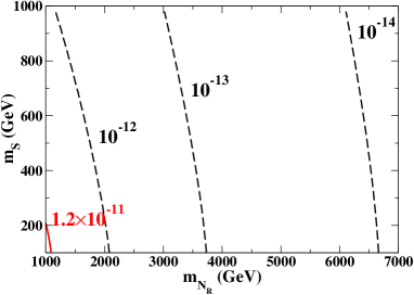
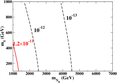
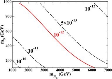
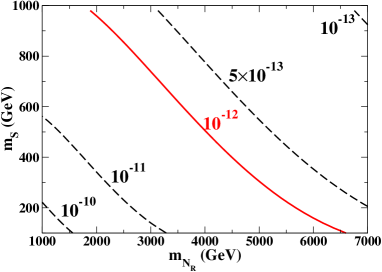
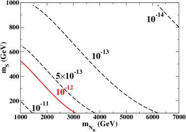
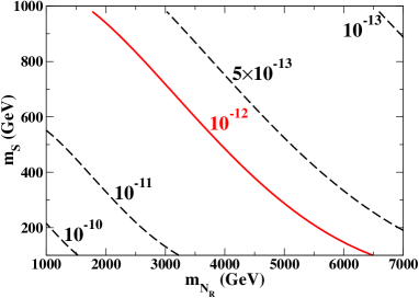
Assuming that heα𝒪(1)similar-tosuperscriptsubscript𝑒𝛼𝒪1h_{e}^{\alpha}\sim{\cal O}(1), the masses of NRαsuperscriptsubscript𝑁𝑅𝛼N_{R}^{\alpha} and S±superscript𝑆plus-or-minusS^{\pm} are strongly constrained from below. In particular, if we assume that mS > 400subscript𝑚𝑆 > 400m_{S}\mbox{ \raisebox{-4.30554pt}{$\stackrel{{\scriptstyle\textstyle>}}{{\textstyle\sim}}$ }}400 GeV, mNR > 𝒪(1)subscript𝑚subscript𝑁𝑅 > 𝒪1m_{N_{R}}\mbox{ \raisebox{-4.30554pt}{$\stackrel{{\scriptstyle\textstyle>}}{{\textstyle\sim}}$ }}{\cal O}(1) TeV is required to satisfy the current experimental bounds, B(μeγ)<1.2×10¹¹𝐵𝜇𝑒𝛾1.2superscript1011B(\mu\rightarrow e\gamma)<1.2\times 10^{-11} MEGA and B(μeee)<1.0×10¹²𝐵𝜇𝑒𝑒𝑒1.0superscript1012B(\mu\rightarrow eee)<1.0\times 10^{-12} meee . Such a relatively heavier S±superscript𝑆plus-or-minusS^{\pm} is favored from the discussion on the dark matter relic abundance and electroweak baryogenesis aks-prl ; aks-prd .

II.4 Typical scenarios

In Table 2, we show four choices for the parameter sets, and resulting values for the neutrino Yukawa coupling constants hiαsuperscriptsubscript𝑖𝛼h_{i}^{\alpha} which satisfy the neutrino data and the LFV data. For all parameter sets, mS=400subscript𝑚𝑆400m_{S}=400 GeV and mNR=5subscript𝑚subscript𝑁𝑅5m_{N_{R}}=5 TeV are assumed. Set A and Set B are taken as the normal hierarchy in the neutrino masses with sin2θ13=0superscript2subscript𝜃130\sin^{2}\theta_{13}=0 and 0.03, respectively, while Set C and Set D are for the inverted hierarchy. The predictions on B(μeγ)𝐵𝜇𝑒𝛾B(\mu\rightarrow e\gamma) and B(μeee)𝐵𝜇𝑒𝑒𝑒B(\mu\rightarrow eee) are also shown in the table333 In Table 2, we show the numbers of the hiαsuperscriptsubscript𝑖𝛼h_{i}^{\alpha} coupling constants with four digits for Set C, because the branching ratios of μeγ𝜇𝑒𝛾\mu\rightarrow e\gamma and μeee𝜇𝑒𝑒𝑒\mu\rightarrow eee are sensitive to these numbers due to large cancellations.. The scenario with the inverted hierarchy requires the larger values for κtanβ𝜅𝛽\kappa\tan\beta, so that the normal hierarchy scenarios are more natural in our model.

Set Inputs Yukawa couplings LFV
sin2θ13superscript2subscript𝜃13\sin^{2}\theta_{13} κtanβ𝜅𝛽\kappa\tan\beta he1superscriptsubscript𝑒1h_{e}^{1} he2superscriptsubscript𝑒2h_{e}^{2} hμ1superscriptsubscript𝜇1h_{\mu}^{1} hμ2superscriptsubscript𝜇2h_{\mu}^{2} hτ1superscriptsubscript𝜏1h_{\tau}^{1} hτ2superscriptsubscript𝜏2h_{\tau}^{2} B(μeγ)𝐵𝜇𝑒𝛾B(\mu\!\!\rightarrow\!\!e\gamma) B(μ3e)𝐵𝜇3𝑒B(\mu\!\!\rightarrow\!\!3e)
A 0 54 1.2 1.3 0.024 -0.011 0.00071 -0.0014 2.8×10142.8superscript10142.8\!\times\!10^{-14} 5.9×10135.9superscript10135.9\!\times\!10^{-13}
B 0.03 76 1.1 1.1 0.0028 0.018 -0.00055 0.00097 6.1×10146.1superscript10146.1\!\times\!10^{-14} 7.4×10137.4superscript10137.4\!\times\!10^{-13}
C 0 80 3.500 3.474 0.01200 -0.01192 -0.0007136 0.0007086 4.4×10174.4superscript10174.4\!\times\!10^{-17} 6.2×10146.2superscript10146.2\!\times\!10^{-14}
D 0.03 128 2.1 2.2 0.0064 -0.0086 -0.00053 0.00035 3.5×10153.5superscript10153.5\!\times\!10^{-15} 7.0×10137.0superscript10137.0\!\times\!10^{-13}
Table 2: Values of hiαsuperscriptsubscript𝑖𝛼h_{i}^{\alpha} as well as those of branching ratios of μeγ𝜇𝑒𝛾\mu\rightarrow e\gamma and μ3e𝜇3𝑒\mu\rightarrow 3e for mη=50subscript𝑚𝜂50m_{\eta}=50 GeV and mH±=100subscript𝑚superscript𝐻plus-or-minus100m_{H^{\pm}}=100 GeV for various scenarios which satisfy neutrino data: Set A and Set B are scenarios of the the normal hierarchy while Set C and Set D are those of the inverted hierarchy. For all sets, mS=400subscript𝑚𝑆400m_{S}=400 GeV and mNR=5subscript𝑚subscript𝑁𝑅5m_{N_{R}}=5 TeV are taken.

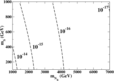
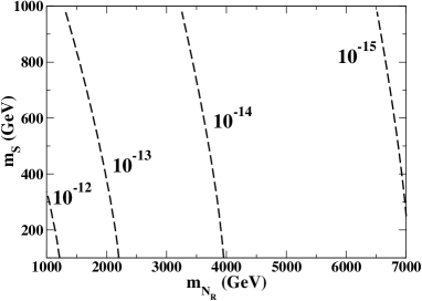
In Fig. 3, the contour plots of the branching ratio B(μeγ)𝐵𝜇𝑒𝛾B(\mu\rightarrow e\gamma) are shown in the mSsubscript𝑚𝑆m_{S}-mNRsubscript𝑚subscript𝑁𝑅m_{N_{R}} plane for the neutrino Yukawa coupling constants in Set A to Set D, while those of the branching ratio B(μeee)𝐵𝜇𝑒𝑒𝑒B(\mu\rightarrow eee) are shown for these scenarios in Fig. 4. The scale of the branching ratio of μeγ𝜇𝑒𝛾\mu\rightarrow e\gamma is determined by mNRsubscript𝑚subscript𝑁𝑅m_{N_{R}} and is insensitive to mSsubscript𝑚𝑆m_{S}, while that of μeee𝜇𝑒𝑒𝑒\mu\rightarrow eee largely depend on both mNRsubscript𝑚subscript𝑁𝑅m_{N_{R}} and mSsubscript𝑚𝑆m_{S} especially for Set A, Set B and Set D. It can easily be seen that a much stronger constraint comes from μeee𝜇𝑒𝑒𝑒\mu\rightarrow eee for all scenarios.

Refer to caption
Refer to caption
Refer to caption
Refer to caption
Figure 3: Contour plots for the branching ratio of μeγ𝜇𝑒𝛾\mu\rightarrow e\gamma for the neutrino Yukawa coupling constants in Set A (top-left), Set B (top-right), Set C (bottom-left) and Set D (bottom-right). The contour for the upper limit from the data is given as the (red) solid curve.
Refer to caption
Refer to caption
Refer to caption
Refer to caption
Figure 4: Contour plots for the branching ratio of μeee𝜇𝑒𝑒𝑒\mu\rightarrow eee for the neutrino Yukawa coupling constants in Set A (top-left), Set B (top-right), Set C (bottom-left) and Set D (bottom-right). The contour for the upper limit from the data is given as the (red) solid curve.

II.5 Dark matter and electroweak phase transition

From now on, we employ Set A in Table 2 for further phenomenological analyses. In this scenario, masses of NRαsuperscriptsubscript𝑁𝑅𝛼N_{R}^{\alpha} are at the multi-TeV scale, so that it may be natural that the rest Z2subscript𝑍2Z_{2}-odd neutral field η𝜂\eta is the candidate of dark matter. Since η𝜂\eta is a singlet under the SM gauge group, the interactions with Z2subscript𝑍2Z_{2}-even particles are only through the Higgs coupling. When mη<mWsubscript𝑚𝜂subscript𝑚𝑊m_{\eta}<m_{W}, the η𝜂\eta field predominantly annihilates into bb¯𝑏¯𝑏b\bar{b} and τ+τsuperscript𝜏superscript𝜏\tau^{+}\tau^{-} through s𝑠s-channel Higgs boson (hh and H𝐻H) mediations. Strong annihilation occurs at mηmH/2similar-to-or-equalssubscript𝑚𝜂subscript𝑚𝐻2m_{\eta}\simeq m_{H}/2 (and mηmh/2similar-to-or-equalssubscript𝑚𝜂subscript𝑚2m_{\eta}\simeq m_{h}/2) due to the resonance of H𝐻H (hh) mediation in the s𝑠s-channel diagrams. The pair annihilation into two photons through one-loop diagrams by H±superscript𝐻plus-or-minusH^{\pm} and S±superscript𝑆plus-or-minusS^{\pm} can also be important if κ𝜅\kappa is of the order one. The relic abundance becomes consistent with the data (ΩDMh20.11similar-tosubscriptΩDMsuperscript20.11\Omega_{\rm DM}h^{2}\sim 0.11 wimp ) for mη5060similar-tosubscript𝑚𝜂5060m_{\eta}\sim 50-60 GeV, when we take mH=mH±100subscript𝑚𝐻subscript𝑚superscript𝐻plus-or-minussimilar-to-or-equals100m_{H}=m_{H^{\pm}}\simeq 100 GeV, mh120similar-to-or-equalssubscript𝑚120m_{h}\simeq 120 GeV, mS > 400subscript𝑚𝑆 > 400m_{S}\mbox{ \raisebox{-4.30554pt}{$\stackrel{{\scriptstyle\textstyle>}}{{\textstyle\sim}}$ }}400 GeV with κ=1.5𝜅1.5\kappa=1.5, σ1=0.05subscript𝜎10.05\sigma_{1}=0.05, σ2=0.03subscript𝜎20.03\sigma_{2}=0.03, and tanβ=36𝛽36\tan\beta=36. In such scenario, the typical spin-independent cross section for the scattering of dark matter with a proton is of order of 108superscript10810^{-8} pb which is within the reach of the direct search experiments such as superCDMS and XMASS.

When mη<mh/2subscript𝑚𝜂subscript𝑚2m_{\eta}<m_{h}/2, the (SM-like) Higgs boson hh can decay into a dark matter pair ηη𝜂𝜂\eta\eta. The branching ratio of hηη𝜂𝜂h\rightarrow\eta\eta is evaluated as 343434 % (222222 %) for mh=120subscript𝑚120m_{h}=120 GeV and mη=48subscript𝑚𝜂48m_{\eta}=48 (555555) GeV when σ1=0.05subscript𝜎10.05\sigma_{1}=0.05, σ2=0.03subscript𝜎20.03\sigma_{2}=0.03 and tanβ>10𝛽10\tan\beta>10. The invisible decay of hh can be tested at the LHC when B(hηη)>25𝐵𝜂𝜂25B(h\rightarrow\eta\eta)>25LHCinv . At the ILC, it is expected that the branching ratio for the invisible decay of a few % can be detected Schumacher:2003ss . Therefore, the invisible decay in this model can be tested at the collider experiments.

Our model aks-prl satisfies the conditions for baryogenesis sakharov . The B𝐵B number violating interaction is the sphaleron interaction. The additional CP violating phases are in the Higgs sector and in the Yukawa interaction. The condition of departure from thermal equilibrium can be realized by the strong first order electroweak phase transition, which requires a large tri-linear coupling of the order parameter in the expression of the high temperature expansion hte where only the bosonic loop can contribute444We note that such a non-decoupling effect due to the bosonic loop can also affect the quantum correction to the triple Higgs boson coupling ewbg-thdm2 ; Ref:KOSY . Such a large correction to the Higgs self-coupling can be an important signature for successful electroweak baryogeneis at collider experiments.. In our model, there are many additional scalars running in the loop so that the large coupling can be easily realized ewbg-thdm2 . The strong first order phase transition is possible for large mSsubscript𝑚𝑆m_{S} and/or mAsubscript𝑚𝐴m_{A} with the large non-decoupling effect: e.g. mS400similar-tosubscript𝑚𝑆400m_{S}\sim 400 GeV, mA100similar-tosubscript𝑚𝐴100m_{A}\sim 100 GeV, M=100𝑀100M=100 GeV and μS=200subscript𝜇𝑆200\mu_{S}=200 GeV, where M𝑀M and μSsubscript𝜇𝑆\mu_{S} are the invariant masses in Eq.(23) and Eq.(27), respectively. The result is not sensitive to tanβ𝛽\tan\beta.

III Bounds from triviality and vacuum stability

There are scalar bosons in this model, so that quadratic divergences appear in the one-loop calculation for their masses. Because there is no mechanism by which such quadratic divergences are eliminated, enormous fine tuning is required to realize the renormalized Higgs boson mass being at the weak scale with a very high cutoff scale. Allowing the 1 % fine tuning, the cutoff scale is at most ΛO(10)similar-toΛ𝑂10\Lambda\sim O(10) TeV, above which the theory would be replaced by a more fundamental one Murayama . Unless a mechanism of cancellation of the quadratic divergences such as supersymmetry is implemented, to avoid excessive fine tuning the model should be regarded as an effective theory, whose cutoff scale ΛΛ\Lambda is between mNRαsubscript𝑚superscriptsubscript𝑁𝑅𝛼m_{N_{R}^{\alpha}} and O(10)𝑂10O(10) TeV. We then need to confirm the theoretical consistency of the model up to ΛΛ\Lambda cabibbo . We here evaluate bounds on the parameter space from vacuum stability and perturbativity, and examine whether the theoretically allowed parameter region is consistent with that by the experimental data discussed in the previous sections.

We have to consider these two bounds seriously because of the following reasons. First, this model includes many scalar fields, e.g.formulae-sequence𝑒𝑔e.g., hh, H𝐻H, A𝐴A, H±superscript𝐻plus-or-minusH^{\pm}, S±superscript𝑆plus-or-minusS^{\pm} and η𝜂\eta, so that the scale dependent dimensionless coupling constants would be drastically changed by the loop corrections due to the scalar bosons. Second, some of the Yukawa coupling constants for right-handed neutrinos are necessarily of order one for a radiative generation of the tiny mass scale of the neutrinos at the three-loop level. Finally, to realize the first order electroweak phase transition, some of the scalar self-coupling constants has to be as large as of order one.

In order to evaluate the vacuum stability bound and the triviality bound, we estimate the scale dependences of the dimensionless coupling constants by using the RGEs at the one-loop level. We have calculated the one-loop beta functions for all the coupling constants in this model. The full set of the beta functions is listed in Appendix. We take into account the threshold effects in the calculation of the scale dependent coupling constants. In the scale below the mass of S±superscript𝑆plus-or-minusS^{\pm}, we treat the theory without NRsubscript𝑁𝑅N_{R} and S±superscript𝑆plus-or-minusS^{\pm}. In the scale between the masses of the S±superscript𝑆plus-or-minusS^{\pm} and NRsubscript𝑁𝑅N_{R}, we treat the theory without NRsubscript𝑁𝑅N_{R}. In the scale higher than the mass of the NRsubscript𝑁𝑅N_{R}, we treat the theory with full particle contents.

III.1 The conditions

In this model, there are scalar fields ΦisubscriptΦ𝑖\Phi_{i} (i=1,2𝑖12i=1,2), S±superscript𝑆plus-or-minusS^{\pm} and η𝜂\eta, which contain eleven degrees of freedom which would share the order parameter. The four of them are eliminated because of the SU(2)L×U(1)Y𝑆𝑈subscript2𝐿𝑈subscript1𝑌SU(2)_{L}\times U(1)_{Y} gauge symmetry. In the remining seven dimensional parameter space, we require that for any direction the potential is bounded from below with keeping positiveness deshpande . In the SM, this requirement is satisfied when the Higgs self-coupling constant is positive. In this model, we put the following conditions on the the dimensionless coupling constants:

λ1(μ)>0,λ2(μ)>0,λS(μ)>0,λη(μ)>0,formulae-sequencesubscript𝜆1𝜇0formulae-sequencesubscript𝜆2𝜇0formulae-sequencesubscript𝜆𝑆𝜇0subscript𝜆𝜂𝜇0\displaystyle\lambda_{1}(\mu)>0,\quad\lambda_{2}(\mu)>0,\quad\lambda_{S}(\mu)>0,\quad\lambda_{\eta}(\mu)>0, (53)
λ1(μ)λ2(μ)+λ3(μ)+MIN[0,(λ4(μ)+λ5(μ)),(λ4(μ)λ5(μ))]>0,subscript𝜆1𝜇subscript𝜆2𝜇subscript𝜆3𝜇MIN0subscript𝜆4𝜇subscript𝜆5𝜇subscript𝜆4𝜇subscript𝜆5𝜇0\displaystyle\sqrt{\lambda_{1}(\mu)\lambda_{2}(\mu)}+\lambda_{3}(\mu)+\text{MIN}[0,\quad(\lambda_{4}(\mu)+\lambda_{5}(\mu)),\quad(\lambda_{4}(\mu)-\lambda_{5}(\mu))]>0,
λ1(μ)λS(μ)/2+ρ1(μ)>0,λ1(μ)λη(μ)/3+σ1(μ)>0,λ2(μ)λS(μ)/2+ρ2(μ)>0,formulae-sequencesubscript𝜆1𝜇subscript𝜆𝑆𝜇2subscript𝜌1𝜇0formulae-sequencesubscript𝜆1𝜇subscript𝜆𝜂𝜇3subscript𝜎1𝜇0subscript𝜆2𝜇subscript𝜆𝑆𝜇2subscript𝜌2𝜇0\displaystyle\sqrt{\lambda_{1}(\mu)\lambda_{S}(\mu)/2}+\rho_{1}(\mu)>0,\quad\sqrt{\lambda_{1}(\mu)\lambda_{\eta}(\mu)/3}+\sigma_{1}(\mu)>0,\quad\sqrt{\lambda_{2}(\mu)\lambda_{S}(\mu)/2}+\rho_{2}(\mu)>0,
λ2(μ)λη(μ)/3+σ2(μ)>0,λS(μ)λη(μ)/6+ξ(μ)>0,formulae-sequencesubscript𝜆2𝜇subscript𝜆𝜂𝜇3subscript𝜎2𝜇0subscript𝜆𝑆𝜇subscript𝜆𝜂𝜇6𝜉𝜇0\displaystyle\sqrt{\lambda_{2}(\mu)\lambda_{\eta}(\mu)/3}+\sigma_{2}(\mu)>0,\quad\sqrt{\lambda_{S}(\mu)\lambda_{\eta}(\mu)/6}+\xi(\mu)>0, (54)
2λ1(μ)+2λ2(μ)+4λ3(μ)+4ρ1(μ)+4ρ2(μ)+λS(μ)+4σ1(μ)+4σ2(μ)2subscript𝜆1𝜇2subscript𝜆2𝜇4subscript𝜆3𝜇4subscript𝜌1𝜇4subscript𝜌2𝜇subscript𝜆𝑆𝜇4subscript𝜎1𝜇4subscript𝜎2𝜇\displaystyle 2\lambda_{1}(\mu)+2\lambda_{2}(\mu)+4\lambda_{3}(\mu)+4\rho_{1}(\mu)+4\rho_{2}(\mu)+\lambda_{S}(\mu)+4\sigma_{1}(\mu)+4\sigma_{2}(\mu)
+23λη(μ)+4ξ(μ)162|κ(μ)|>0.23subscript𝜆𝜂𝜇4𝜉𝜇162𝜅𝜇0\displaystyle+\frac{2}{3}\lambda_{\eta}(\mu)+4\xi(\mu)-16\sqrt{2}|\kappa(\mu)|>0. (55)

The conditions in Eqs. (53) and (54) are obtained by the similar way as in Ref. kkloy , while the last condition in Eq. (55) is derived such that the term with the coupling constant κ𝜅\kappa in the potential satisfies the positivity condition for the direction where the VEVs of the fields Φ1subscriptΦ1\Phi_{1}, Φ2subscriptΦ2\Phi_{2}, S±superscript𝑆plus-or-minusS^{\pm} and η𝜂\eta are a common value.

We require that all the dimensionless running coupling constants do not blow up below ΛΛ\Lambda. Since we discuss the model within the scale where the perturbation calculation remains reliable, we here require that the running coupling constants do not exceed some critical value. In this paper, we impose the following criterion in the coupling constants in the Higgs potential Eq. (3) and the Yukawa interaction in Eqs. (1) and (2):

|λi(μ)|,|σi(μ)|,|ρi(μ)|,|κ(μ)|,|ξ(μ)|<8π,subscript𝜆𝑖𝜇subscript𝜎𝑖𝜇subscript𝜌𝑖𝜇𝜅𝜇𝜉𝜇8𝜋\displaystyle|\lambda_{i}(\mu)|,\hskip 5.69054pt|\sigma_{i}(\mu)|,\hskip 5.69054pt|\rho_{i}(\mu)|,\hskip 5.69054pt|\kappa(\mu)|,\hskip 5.69054pt|\xi(\mu)|<8\pi,
yt2(μ),yb2(μ),yτ2(μ),(hiα)2(μ)<4π.superscriptsubscript𝑦𝑡2𝜇superscriptsubscript𝑦𝑏2𝜇superscriptsubscript𝑦𝜏2𝜇superscriptsuperscriptsubscript𝑖𝛼2𝜇4𝜋\displaystyle y_{t}^{2}(\mu),\hskip 5.69054pty_{b}^{2}(\mu),\hskip 5.69054pty_{\tau}^{2}(\mu),\hskip 5.69054pt(h_{i}^{\alpha})^{2}(\mu)<4\pi. (56)

The similar critical value has been adopted in the analyses in the two Higgs dobulet model vs_thdm and in the Zee model kkloy .

III.2 Allowed regions in the parameter space

In this section, we evaluate allowed regions in parameter space, which satisfy the conditions of triviality and vacuum stability for each fixed cutoff scale ΛΛ\Lambda. For the scenarios of the neutrino Yukawa coupling constants as well as the masses of right-handed neutrinos, we choose Set A in Table 2. We investigate the allowed regions in the mSsubscript𝑚𝑆m_{S}-mAsubscript𝑚𝐴m_{A} plane, and the rest of the mass parameters in the scalar sector is fixed as shown in Teble 3.

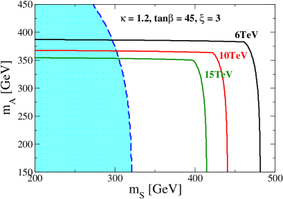
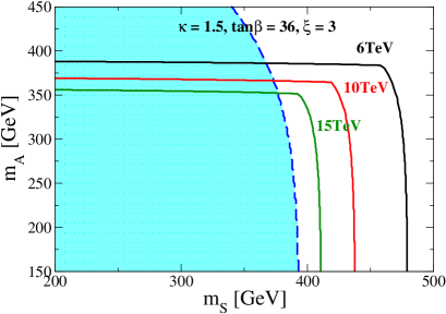
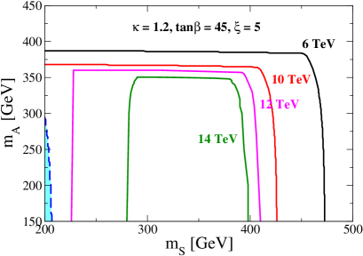
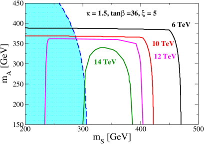
The initial values for the scalar coupling constants in the Higgs sector are shown in Table. 4. We note that the initial value of λ4subscript𝜆4\lambda_{4}, λ5subscript𝜆5\lambda_{5} and ρ2subscript𝜌2\rho_{2} are determined by given values for the masses of A𝐴A and S±superscript𝑆plus-or-minusS^{\pm} using Eqs. (23), (24) and (27). The rest parameter ξ𝜉\xi (the coupling constant for |S|2η2superscriptsuperscript𝑆2superscript𝜂2|S^{-}|^{2}\eta^{2}) is taken as ξ=3𝜉3\xi=3 and 555. The results in the case with ξ=3𝜉3\xi=3 is shown in Fig. 6 for κ=1.2𝜅1.2\kappa=1.2 (left figure) and κ=1.5𝜅1.5\kappa=1.5 (right figure), while those with ξ=5𝜉5\xi=5 is in Fig. 6 for the same values of κ𝜅\kappa.

In Fig. 6, the shaded area in the figure is excluded due to the vacuum stability condition in Eq. (55). In this area, the condition is not satisfied already at the electroweak scale, so that the excluded region is independent of ΛΛ\Lambda. The vacuum stability bound become stronger for a larger value of κ𝜅\kappa, although the area compatible with both theoretical conditions with Λ=10Λ10\Lambda=10 TeV still exists for κ=1.5𝜅1.5\kappa=1.5. On the other hand, the bound from perturbativity depends on ΛΛ\Lambda. In Fig. 6, the contour plots for Λ=6Λ6\Lambda=6, 101010 and 151515 TeV, the scales where one of the coupling constants blows up and breaks the condition of perturbativity are shown for the case of ξ=3𝜉3\xi=3 in the mSsubscript𝑚𝑆m_{S}-mAsubscript𝑚𝐴m_{A} plane. We find that there is the parameter region which satisfies both the conditions of vacuum stability and perturbativity with the blow-up scale to be above Λ=10Λ10\Lambda=10 TeV. The area of the vicinity of mS400similar-tosubscript𝑚𝑆400m_{S}\sim 400 GeV and mA<350subscript𝑚𝐴350m_{A}<350 GeV can also be consistent from the theoretical bounds. We stress that this parameter region is favored for phenomenologically successful scenarios for neutrino masses, relic abundance for the dark matter, and the strongly first order phase transition.

The similar figures but with ξ=5𝜉5\xi=5 are shown in Fig. 6. The contour plots are for Λ=6Λ6\Lambda=6, 101010, 121212 and 141414 TeV in the mSsubscript𝑚𝑆m_{S}-mAsubscript𝑚𝐴m_{A} plane. We find that there is the parameter region which satisfies both the conditions of vacuum stability and perturbativity with the blow-up scale to be above Λ=10Λ10\Lambda=10 TeV. The vacuum stability bound is more relaxed as compared to that for ξ=3𝜉3\xi=3, while the bound from perturbatibity becomes rather strict. In the regions with mS<400subscript𝑚𝑆400m_{S}<400 GeV, the running coupling constants blow up earlier than the case with ξ=3𝜉3\xi=3, because of the threshold effect at the scale μ=mS𝜇subscript𝑚𝑆\mu=m_{S}, above which the running of ληsubscript𝜆𝜂\lambda_{\eta} becomes enhanced by the loop contribution of S±superscript𝑆plus-or-minusS^{\pm}. In the area of 300300300 GeV <mS<400absentsubscript𝑚𝑆400<m_{S}<400 GeV and mA<350subscript𝑚𝐴350m_{A}<350 GeV, ΛΛ\Lambda can be above 101010 TeV.

Masses (GeV) Inv. masses (GeV)
mH±superscriptsubscript𝑚𝐻plus-or-minusm_{H}^{\pm} mHsubscript𝑚𝐻m_{H} mhsubscript𝑚m_{h} mηsubscript𝑚𝜂m_{\eta} M𝑀M μSsubscript𝜇𝑆\mu_{S} μηsubscript𝜇𝜂\mu_{\eta}
100 100 120 50 100 200 30
Table 3: Values for the scalar boson masses and the invariant mass parameters.
Scalar couplings
λ1(mZ)subscript𝜆1subscript𝑚𝑍\lambda_{1}(m_{Z}) λ2(mZ)subscript𝜆2subscript𝑚𝑍\lambda_{2}(m_{Z}) λ3(mZ)subscript𝜆3subscript𝑚𝑍\lambda_{3}(m_{Z}) κ(mS)tanβ𝜅subscript𝑚𝑆𝛽\kappa(m_{S})\tan\beta ρ1(mS)subscript𝜌1subscript𝑚𝑆\rho_{1}(m_{S}) λS(mS)subscript𝜆𝑆subscript𝑚𝑆\lambda_{S}(m_{S}) σ1(mZ)subscript𝜎1subscript𝑚𝑍\sigma_{1}(m_{Z}) σ2(mZ)subscript𝜎2subscript𝑚𝑍\sigma_{2}(m_{Z}) λη(mZ)subscript𝜆𝜂subscript𝑚𝑍\lambda_{\eta}(m_{Z}) sin(βα)𝛽𝛼\sin(\beta-\alpha)
0.24 0.24 0.24 54 0.1 2 0.05 0.05 3 1
Table 4: Values for the scalar coupling constants and the mixing angles.
Refer to caption
Refer to caption
Figure 5: Contour plots for the scale where condition of perturbativity is broken are shown in the mSsubscript𝑚𝑆m_{S}-mAsubscript𝑚𝐴m_{A} plane in the case of (κ,tanβ)=(1.2,45)𝜅𝛽1.245(\kappa,\tan\beta)=(1.2,45) (left figure), and (κ,tanβ)=(1.5,36)𝜅𝛽1.536(\kappa,\tan\beta)=(1.5,36) (right figure). The region excluded by the vacuum stability condition is also shown as the shaded area. The constant ξ𝜉\xi is taken to be 3 at the scale of mSsubscript𝑚𝑆m_{S}.
Refer to caption
Refer to caption
Figure 6: Contour plots for the scale where condition of perturbativity is broken are shown in the mSsubscript𝑚𝑆m_{S}-mAsubscript𝑚𝐴m_{A} plane in the case of (κ,tanβ)=(1.2,45)𝜅𝛽1.245(\kappa,\tan\beta)=(1.2,45) (left figure), and (κ,tanβ)=(1.5,36)𝜅𝛽1.536(\kappa,\tan\beta)=(1.5,36) (right figure). The region excluded by the vacuum stability condition is also shown as the shaded area. The constant ξ𝜉\xi is taken to be 5 at the scale of mSsubscript𝑚𝑆m_{S}.

IV Conclusion

We have discussed theoretical constraints on the parameter space under the conditions from vacuum stability and triviality in the three-loop radiative seesaw model with TeV-scale right-handed neutrinos which are odd under the Z2subscript𝑍2Z_{2} parity. It has been found that the model can be consistent up to the scale above 10 TeV in the parameter region which satisfies the neutrino data, the LFV data, the thermal relic abundance of dark matter as well as the requrement from the strongly first order phase transiton. We also reanalyzed the constraint from the LFV data. The data from μeee𝜇𝑒𝑒𝑒\mu\rightarrow eee is found to be more severer than that from μeγ𝜇𝑒𝛾\mu\rightarrow e\gamma. Our analysis here has been restricted in the case where the CP violation is neglected just for simplicity. The analysis for consistency with including the CP violating phase, which is necessary for finally producing the observed asymmetry of baryon number at the electroweak phase transition, will be done in near future.

Acknowledgments

The work of MA was supported in part by Grant-in-Aid for Young Scientists (B) no. 22740137, that of SK was supported in part by Grant-in-Aid for Scientific Research (A) no. 22244031 and (C) no. 19540277, that of KY was supported by Japan Society for the Promotion of Science (JSPS Fellow (DC2)).

Appendix

The full set of the beta functions for RGEs in the model in Ref. aks-prl is given at the one-loop level by

β(gs)𝛽subscript𝑔𝑠\displaystyle\beta(g_{s}) =116π2[7gs3],absent116superscript𝜋2delimited-[]7superscriptsubscript𝑔𝑠3\displaystyle=\frac{1}{16\pi^{2}}\left[-7g_{s}^{3}\right], (57)
β(g)𝛽𝑔\displaystyle\beta(g) =116π2[3g3],absent116superscript𝜋2delimited-[]3superscript𝑔3\displaystyle=\frac{1}{16\pi^{2}}\left[-3g^{3}\right], (58)
β(g)𝛽superscript𝑔\displaystyle\beta(g^{\prime}) =116π2[223g3],\displaystyle=\frac{1}{16\pi^{2}}\Big{[}-\frac{22}{3}g^{{}^{\prime}3}\Big{]}, (59)
β(yt)𝛽subscript𝑦𝑡\displaystyle\beta(y_{t}) =116π2[8ytgs294g2yt1712g2yt+92yt3+32ytyb2],\displaystyle=\frac{1}{16\pi^{2}}\Big{[}-8y_{t}g_{s}^{2}-\frac{9}{4}g^{2}y_{t}-\frac{17}{12}g^{{}^{\prime}2}y_{t}+\frac{9}{2}y_{t}^{3}+\frac{3}{2}y_{t}y_{b}^{2}\Big{]}, (60)
β(yb)𝛽subscript𝑦𝑏\displaystyle\beta(y_{b}) =116π2[8ytgs294g2yt512g2yt+92yb3+32yt2yb],\displaystyle=\frac{1}{16\pi^{2}}\Big{[}-8y_{t}g_{s}^{2}-\frac{9}{4}g^{2}y_{t}-\frac{5}{12}g^{{}^{\prime}2}y_{t}+\frac{9}{2}y_{b}^{3}+\frac{3}{2}y_{t}^{2}y_{b}\Big{]}, (61)
β(yτ)𝛽subscript𝑦𝜏\displaystyle\beta(y_{\tau}) =116π2[94g2yτ154g2yτ+52yτ3],\displaystyle=\frac{1}{16\pi^{2}}\Big{[}-\frac{9}{4}g^{2}y_{\tau}-\frac{15}{4}g^{{}^{\prime}2}y_{\tau}+\frac{5}{2}y_{\tau}^{3}\Big{]}, (62)
β(hiα)𝛽superscriptsubscript𝑖𝛼\displaystyle\beta(h_{i}^{\alpha}) =116π2[5g2hiα+12hiαj(hjα)2+12hiαβ(hiβ)2+hiαj,β(hjβ)2],\displaystyle=\frac{1}{16\pi^{2}}\Big{[}-5g^{{}^{\prime}2}h_{i}^{\alpha}+\frac{1}{2}h_{i}^{\alpha}\sum_{j}(h_{j}^{\alpha})^{2}+\frac{1}{2}h_{i}^{\alpha}\sum_{\beta}(h_{i}^{\beta})^{2}+h_{i}^{\alpha}\sum_{j,\beta}(h_{j}^{\beta})^{2}\Big{]}, (63)
β(λ1)𝛽subscript𝜆1\displaystyle\beta(\lambda_{1}) =116π2[12λ12+4λ32+2λ42+2λ52+4λ3λ4+2ρ12+σ12+94g4+64g2g2+34g4\displaystyle=\frac{1}{16\pi^{2}}\Big{[}12\lambda_{1}^{2}+4\lambda_{3}^{2}+2\lambda_{4}^{2}+2\lambda_{5}^{2}+4\lambda_{3}\lambda_{4}+2\rho_{1}^{2}+\sigma_{1}^{2}+\frac{9}{4}g^{4}+\frac{6}{4}g^{2}g^{{}^{\prime}2}+\frac{3}{4}g^{{}^{\prime}4}
4yτ4+(4yτ29g23g2)λ1],\displaystyle\hskip 42.67912pt-4y_{\tau}^{4}+(4y_{\tau}^{2}-9g^{2}-3g^{{}^{\prime}2})\lambda_{1}\Big{]}, (64)
β(λ2)𝛽subscript𝜆2\displaystyle\beta(\lambda_{2}) =116π2[12λ22+4λ32+2λ42+2λ52+4λ3λ4+2ρ22+σ22+94g4+64g2g2+34g4\displaystyle=\frac{1}{16\pi^{2}}\Big{[}12\lambda_{2}^{2}+4\lambda_{3}^{2}+2\lambda_{4}^{2}+2\lambda_{5}^{2}+4\lambda_{3}\lambda_{4}+2\rho_{2}^{2}+\sigma_{2}^{2}+\frac{9}{4}g^{4}+\frac{6}{4}g^{2}g^{{}^{\prime}2}+\frac{3}{4}g^{{}^{\prime}4}
12yt412yb4+(12yt2+12yb29g23g2)λ2],\displaystyle\hskip 42.67912pt-12y_{t}^{4}-12y_{b}^{4}+(12y_{t}^{2}+12y_{b}^{2}-9g^{2}-3g^{{}^{\prime}2})\lambda_{2}\Big{]}, (65)
β(λ3)𝛽subscript𝜆3\displaystyle\beta(\lambda_{3}) =116π2[6λ1λ3+2λ1λ4+6λ2λ3+2λ2λ4+4λ32+2λ42+2λ52+2ρ1ρ2+σ1σ2+4κ2\displaystyle=\frac{1}{16\pi^{2}}\Big{[}6\lambda_{1}\lambda_{3}+2\lambda_{1}\lambda_{4}+6\lambda_{2}\lambda_{3}+2\lambda_{2}\lambda_{4}+4\lambda_{3}^{2}+2\lambda_{4}^{2}+2\lambda_{5}^{2}+2\rho_{1}\rho_{2}+\sigma_{1}\sigma_{2}+4\kappa^{2}
+94g4+34g464g2g2+(6yt2+6yb2+2yτ29g23g2)λ3],\displaystyle\hskip 42.67912pt+\frac{9}{4}g^{4}+\frac{3}{4}g^{{}^{\prime}4}-\frac{6}{4}g^{2}g^{{}^{\prime}2}+(6y_{t}^{2}+6y_{b}^{2}+2y_{\tau}^{2}-9g^{2}-3g^{{}^{\prime}2})\lambda_{3}\Big{]}, (66)
β(λ4)𝛽subscript𝜆4\displaystyle\beta(\lambda_{4}) =116π2[2(λ1+λ2+4λ3+2λ4)λ4+8λ528κ2+3g2g2.\displaystyle=\frac{1}{16\pi^{2}}\Big{[}2(\lambda_{1}+\lambda_{2}+4\lambda_{3}+2\lambda_{4})\lambda_{4}+8\lambda_{5}^{2}-8\kappa^{2}+3g^{2}g^{{}^{\prime}2}\Big{.}
.+(6yt2+6yb2+2yτ29g23g2)λ4],\displaystyle\hskip 56.9055pt\Big{.}+(6y_{t}^{2}+6y_{b}^{2}+2y_{\tau}^{2}-9g^{2}-3g^{{}^{\prime}2})\lambda_{4}\Big{]}, (67)
β(λ5)𝛽subscript𝜆5\displaystyle\beta(\lambda_{5}) =116π2[2(λ1+λ2+4λ3+6λ4)λ5+(6yt2+6yb2+2yτ29g23g2)λ5]\displaystyle=\frac{1}{16\pi^{2}}\Big{[}2(\lambda_{1}+\lambda_{2}+4\lambda_{3}+6\lambda_{4})\lambda_{5}+(6y_{t}^{2}+6y_{b}^{2}+2y_{\tau}^{2}-9g^{2}-3g^{{}^{\prime}2})\lambda_{5}\Big{]} (68)
β(ρ1)𝛽subscript𝜌1\displaystyle\beta(\rho_{1}) =116π2[6λ1ρ1+4λ3ρ2+2λ4ρ2+2ρ1λS+4ρ12+σ1ξ+8κ2+3g4\displaystyle=\frac{1}{16\pi^{2}}\Big{[}6\lambda_{1}\rho_{1}+4\lambda_{3}\rho_{2}+2\lambda_{4}\rho_{2}+2\rho_{1}\lambda_{S}+4\rho_{1}^{2}+\sigma_{1}\xi+8\kappa^{2}+3g^{{}^{\prime}4}
+(152g292g2+2i,α(hiα)2+2yτ2)ρ1],\displaystyle\hskip 42.67912pt+(-\frac{15}{2}g^{{}^{\prime}2}-\frac{9}{2}g^{2}+2\sum_{i,\alpha}(h_{i}^{\alpha})^{2}+2y_{\tau}^{2})\rho_{1}\Big{]}, (69)
β(ρ2)𝛽subscript𝜌2\displaystyle\beta(\rho_{2}) =116π2[6λ2ρ2+4λ3ρ1+2λ4ρ1+2ρ2λS+4ρ22+σ2ξ+8κ2+3g4\displaystyle=\frac{1}{16\pi^{2}}\Big{[}6\lambda_{2}\rho_{2}+4\lambda_{3}\rho_{1}+2\lambda_{4}\rho_{1}+2\rho_{2}\lambda_{S}+4\rho_{2}^{2}+\sigma_{2}\xi+8\kappa^{2}+3g^{{}^{\prime}4}
+(152g292g2+2i,α(hiα)2+6yt2+6yb2)ρ2],\displaystyle\hskip 42.67912pt+(-\frac{15}{2}g^{{}^{\prime}2}-\frac{9}{2}g^{2}+2\sum_{i,\alpha}(h_{i}^{\alpha})^{2}+6y_{t}^{2}+6y_{b}^{2})\rho_{2}\Big{]}, (70)
β(λS)𝛽subscript𝜆𝑆\displaystyle\beta(\lambda_{S}) =116π2[8ρ12+8ρ22+5λS2+2ξ2+24g412g2λS.\displaystyle=\frac{1}{16\pi^{2}}\Big{[}8\rho_{1}^{2}+8\rho_{2}^{2}+5\lambda_{S}^{2}+2\xi^{2}+24g^{{}^{\prime}4}-12g^{{}^{\prime}2}\lambda_{S}\Big{.}
.+4i,α(hiα)2λS8i,jα,βhiαhiβhjβhjα],\displaystyle\Big{.}\hskip 56.9055pt+4\sum_{i,\alpha}(h_{i}^{\alpha})^{2}\lambda_{S}-8\sum_{i,j}\sum_{\alpha,\beta}h_{i}^{\alpha}h_{i}^{\beta}h_{j}^{\beta}h_{j}^{\alpha}\Big{]}, (71)
β(σ1)𝛽subscript𝜎1\displaystyle\beta(\sigma_{1}) =116π2[6λ1σ1+(4λ3+2λ4)σ2+σ1λη+2ρ1ξ+16κ2+(92g232g2+2yτ2)σ1],\displaystyle=\frac{1}{16\pi^{2}}\Big{[}6\lambda_{1}\sigma_{1}+(4\lambda_{3}+2\lambda_{4})\sigma_{2}+\sigma_{1}\lambda_{\eta}+2\rho_{1}\xi+16\kappa^{2}+(-\frac{9}{2}g^{2}-\frac{3}{2}g^{{}^{\prime}2}+2y_{\tau}^{2})\sigma_{1}\Big{]}, (72)
β(σ2)𝛽subscript𝜎2\displaystyle\beta(\sigma_{2}) =116π2[6λ2σ2+(4λ3+2λ4)σ1+σ2λη+2ρ2ξ+16κ2.\displaystyle=\frac{1}{16\pi^{2}}\Big{[}6\lambda_{2}\sigma_{2}+(4\lambda_{3}+2\lambda_{4})\sigma_{1}+\sigma_{2}\lambda_{\eta}+2\rho_{2}\xi+16\kappa^{2}\Big{.}
.+(92g232g2+6yt2+6yb2)σ2],\displaystyle\hskip 56.9055pt\Big{.}+(-\frac{9}{2}g^{2}-\frac{3}{2}g^{{}^{\prime}2}+6y_{t}^{2}+6y_{b}^{2})\sigma_{2}\Big{]}, (73)
β(λη)𝛽subscript𝜆𝜂\displaystyle\beta(\lambda_{\eta}) =116π2[12(σ12+σ22)+3λη2+6ξ2],absent116superscript𝜋2delimited-[]12superscriptsubscript𝜎12superscriptsubscript𝜎223superscriptsubscript𝜆𝜂26superscript𝜉2\displaystyle=\frac{1}{16\pi^{2}}\Big{[}12(\sigma_{1}^{2}+\sigma_{2}^{2})+3\lambda_{\eta}^{2}+6\xi^{2}\Big{]}, (74)
β(κ)𝛽𝜅\displaystyle\beta(\kappa) =116π2κ[2λ32λ4+2ξ+2σ1+2σ2+2ρ1+2ρ2+α,i(hiα)2.\displaystyle=\frac{1}{16\pi^{2}}\kappa\Big{[}2\lambda_{3}-2\lambda_{4}+2\xi+2\sigma_{1}+2\sigma_{2}+2\rho_{1}+2\rho_{2}+\sum_{\alpha,i}(h_{i}^{\alpha})^{2}\Big{.}
.92g292g2+3yt2+3yb2+yτ2],\displaystyle\hskip 56.9055pt\Big{.}-\frac{9}{2}g^{2}-\frac{9}{2}g^{{}^{\prime}2}+3y_{t}^{2}+3y_{b}^{2}+y_{\tau}^{2}\Big{]}, (75)
β(ξ)𝛽𝜉\displaystyle\beta(\xi) =116π2[4ρ1σ1+4ρ2σ2+2λSξ+ληξ+4ξ26g2ξ+2α,i(hiα)2ξ].\displaystyle=\frac{1}{16\pi^{2}}\Big{[}4\rho_{1}\sigma_{1}+4\rho_{2}\sigma_{2}+2\lambda_{S}\xi+\lambda_{\eta}\xi+4\xi^{2}-6g^{{}^{\prime}2}\xi+2\sum_{\alpha,i}(h_{i}^{\alpha})^{2}\xi\Big{]}. (76)

References

  • (1) M. C. Bento, O. Bertolami, R. Rosenfeld and L. Teodoro, Phys. Rev.  D 62, 041302 (2000).
  • (2) X. G. He, T. Li, X. Q. Li, J. Tandean and H. C. Tsai, Phys. Lett.  B 688, 332 (2010); M. Farina, D. Pappadopulo and A. Strumia, Phys. Lett.  B 688, 329 (2010); K. Cheung and T. C. Yuan, Phys. Lett.  B 685, 182 (2010); S. Kanemura, S. Matsumoto, T. Nabeshima and N. Okada, Phys. Rev.  D 82, 055026 (2010).
  • (3) A. Zee, Phys. Lett.  B 93, 389 (1980) [Erratum-ibid.  B 95, 461 (1980)]; A. Zee, Phys. Lett.  B 161, 141 (1985).
  • (4) A. Zee, Nucl. Phys. B 264, 99 (1986); K. S. Babu, Phys. Lett. B 203, 132 (1988).
  • (5) L. M. Krauss, S. Nasri and M. Trodden, Phys. Rev.  D 67, 085002 (2003).
  • (6) E. Ma, Phys. Rev.  D 73, 077301 (2006).
  • (7) M. Aoki, S. Kanemura and O. Seto, Phys. Rev. Lett.  102, 051805 (2009).
  • (8) A. D. Sakharov, Pisma Zh. Eksp. Teor. Fiz.  5, 32 (1967).
  • (9) e.g., A. G. Cohen, D. B. Kaplan and A. E. Nelson, Ann. Rev. Nucl. Part. Sci.  43, 27 (1993); M. Quiros, Helv. Phys. Acta 67, 451 (1994);  V. A. Rubakov and M. E. Shaposhnikov, Usp. Fiz. Nauk 166, 493 (1996) [Phys. Usp.  39, 461 (1996)].
  • (10) J. Kubo, E. Ma and D. Suematsu, Phys. Lett.  B 642, 18 (2006); T. Hambye, K. Kannike, E. Ma and M. Raidal, Phys. Rev.  D 75, 095003 (2007); D. Aristizabal Sierra, J. Kubo, D. Restrepo, D. Suematsu and O. Zapata, Phys. Rev.  D 79, 013011 (2009).
  • (11) S. Kanemura, T. Kasai, G. L. Lin, Y. Okada, J. J. Tseng and C. P. Yuan, Phys. Rev.  D 64, 053007 (2001).
  • (12) K. S. Babu and C. Macesanu, Phys. Rev. D 67, 073010 (2003); D. Aristizabal Sierra and M. Hirsch, JHEP 0612, 052 (2006); M. Nebot, J. F. Oliver, D. Palao and A. Santamaria, Phys. Rev.  D 77, 093013 (2008).
  • (13) M. Aoki, S. Kanemura, T. Shindou and K. Yagyu, JHEP 1007, 084 (2010).
  • (14) K. Cheung and O. Seto, Phys. Rev.  D 69, 113009 (2004).
  • (15) E. Ma, Phys. Lett.  B 662, 49 (2008); E. Ma, Mod. Phys. Lett.  A 23, 721 (2008); R. A. Porto and A. Zee, Phys. Rev.  D 79, 013003 (2009); E. Ma and D. Suematsu, Mod. Phys. Lett.  A 24, 583 (2009).
  • (16) Q. H. Cao, E. Ma and G. Rajasekaran, Phys. Rev.  D 76, 095011 (2007).
  • (17) S. Kanemura, Y. Okada and E. Senaha, Phys. Lett.  B 606, 361 (2005).
  • (18) M. Aoki, S. Kanemura and O. Seto, Phys. Rev.  D 80, 033007 (2009).
  • (19) M. Aoki, S. Kanemura, K. Tsumura and K. Yagyu, Phys. Rev.  D 80, 015017 (2009).
  • (20) A. Belyaev, R. Guedes, S. Moretti and R. Santos, JHEP 1007, 051 (2010).
  • (21) M. Aoki and S. Kanemura, Phys. Lett. B 689, 28 (2010).
  • (22) M. Aoki, S. Kanemura and O. Seto, Phys. Lett. B 685, 313 (2010).
  • (23) N. Cabibbo, L. Maiani, G. Parisi and R. Petronzio, Nucl. Phys.  B 158, 295 (1979); K. Inoue, A. Kakuto, H. Komatsu and S. Takeshita, Prog. Theor. Phys.  67, 1889 (1982); H. Komatsu, Prog. Theor. Phys.  67, 1177 (1982).
  • (24) C. F. Kolda, and H. Murayama, JHEP 0007, 035 (2000).
  • (25) S. Kanemura, T. Kubota and E. Takasugi, Phys. Lett.  B 313, 155 (1993); A. G. Akeroyd, A. Arhrib and E. M. Naimi, Phys. Lett.  B 490, 119 (2000); I. F. Ginzburg and I. P. Ivanov, Phys. Rev.  D 72, 115010 (2005).
  • (26) S. Nie and M. Sher, Phys. Lett.  B 449, 89 (1999); S. Kanemura, T. Kasai and Y. Okada, Phys. Lett.  B 471, 182 (1999).
  • (27) U. Bellgardt et al. [SINDRUM Collaboration], Nucl. Phys. B 299, 1 (1988).
  • (28) M. L. Brooks et al. [MEGA Collaboration], Phys. Rev. Lett.  83, 1521 (1999).
  • (29) S. L. Glashow and S. Weinberg, Phys. Rev.  D 15, 1958 (1977).
  • (30) V. D. Barger, J. L. Hewett and R. J. N. Phillips, Phys. Rev.  D 41, 3421 (1990).
  • (31) Y. Grossman, Nucl. Phys.  B 426, 355 (1994).
  • (32) H. S. Goh, L. J. Hall and P. Kumar, JHEP 0905, 097 (2009); S. Su and B. Thomas, Phys. Rev.  D 79, 095014 (2009); H. E. Logan and D. MacLennan, Phys. Rev.  D 79, 115022 (2009).
  • (33) G. Passarino and M. J. G. Veltman, Nucl. Phys.  B 160, 151 (1979).
  • (34) Z. Maki, M. Nakagawa and S. Sakata, Prog. Theor. Phys.  28, 870 (1962).
  • (35) K. Nakamura et al. (Particle Data Group), J. Phys. G 37, 075021 (2010).
  • (36) E. Komatsu et al. [WMAP Collaboration], Astrophys. J. Suppl.  180, 330 (2009).
  • (37) Di Girolamo and B, Neukermans, L 2003 Atlas Note ATL-PHYS-2003-006; M. Warsinsky [ATLAS Collaboration], J. Phys. Conf. Ser.  110, 072046 (2008).
  • (38) M. Schumacher, Repot No. LC-PHSM-2003-096.
  • (39) G. W. Anderson and L. J. Hall, Phys. Rev.  D 45, 2685 (1992); M. Dine, R. G. Leigh, P. Y. Huet, A. D. Linde and D. A. Linde, Phys. Rev.  D 46, 550 (1992).
  • (40) S. Kanemura, S. Kiyoura, Y. Okada, E. Senaha and C. P. Yuan, Phys. Lett.  B 558, 157 (2003); S. Kanemura, Y. Okada, E. Senaha and C. P. Yuan, Phys. Rev.  D 70, 115002 (2004).
  • (41) N. G. Deshpande and E. Ma, Phys. Rev.  D 18, 2574 (1978).