Detecting Separation in Robotic and Sensor Networks
Abstract
In this paper we consider the problem of monitoring detecting separation of agents from a base station in robotic and sensor networks. Such separation can be caused by mobility and/or failure of the agents. While separation/cut detection may be performed by passing messages between a node and the base in static networks, such a solution is impractical for networks with high mobility, since routes are constantly changing. We propose a distributed algorithm to detect separation from the base station. The algorithm consists of an averaging scheme in which every node updates a scalar state by communicating with its current neighbors. We prove that if a node is permanently disconnected from the base station, its state converges to . If a node is connected to the base station in an average sense, even if not connected in any instant, then we show that the expected value of its state converges to a positive number. Therefore, a node can detect if it has been separated from the base station by monitoring its state. The effectiveness of the proposed algorithm is demonstrated through simulations, a real system implementation and experiments involving both static as well as mobile networks.
keywords:
mobile ad-hoc network , robotic network , sensor network , fault detection1 Introduction
Sensor and robotic networks is a quickly developing area extending the boundaries of traditional robotics and usual sensor networks [1, 2]. In such a network, static as well as mobile nodes (robots) with varying levels of sensing, communication and actuation capability are used to observe, monitor, and control the state of physical processes. For example, in a scenario depicted in Figure 1, a team of ground robots may serve as information aggregators from a large number of static sensors deployed in an area as well as relays to send the processed data to more maneuverable autonomous aerial vehicles. We refer to all the devices that take part in sharing information, whether static or mobile as nodes or agents. Thus in Figure 1 the agents are the chopper, the mobile ground vehicles and the static sensors.

The communication topology of a robotic and sensor network is likely to change over time. Such changes can occur not only due to the mobility of the robotic nodes, but are also likely with static agents due to failures. An agent may fail due to various factors such as mechanical/electrical problems, environmental degradation, battery depletion, or hostile tampering. These causes are especially common for networks deployed in harsh and dangerous situations for applications such as forest fire monitoring, battlefield or emergency response operations [3].
Information exchange through wireless communication is a crucial ingredient for a sensor and robotic network system to carry out the tasks it is deployed for. Long range information exchange between agents is usually achieved by multi-hop wireless communication. In mobile networks, it is quite possible that the agents get separated into two or more sub-networks with no paths for data routing among these sub-networks. We say that a cut has occurred in such an event. A node that is disconnected from the base station at some time may also get reconnected later, e.g., when a mobile node moves in such a way that it restores connectivity between two disconnected sets of agents. In a robotic and sensor network, cuts can occur and disappear due to a combination of node mobility and node failure.
Multi-hop transmission typically requires routing data from a source node to a sink node, which is usually the base station. In a network with highly dynamic topology – common for sensor and robotic networks - maintaining updated routing tables, or discovering routing paths on demand, are challenging and energy inefficient tasks [4]. In such situations, sometimes information transfer from a node to a base station is accomplished by waiting till the node comes within range of the base station or to another node that is close to the base station [5]. In either scenario, it is imperative for the agents to know if a cut occurs, so necessary action can be taken. For example, once a cut is detected, mobile robots can attempt to heal the network by repositioning themselves or placing new communication relay nodes in critical regions. There are other advantages of an ability to detect separation from the base. If a node that is separated from the base station initiates data transmission to the base station, it will only lead to wastage of precious on-board energy of itself and its nearby nodes that attempt to route the packets to the base station, since no path to the destination exists. Therefore, after a cut occurs it is better for such nodes not to initiate any long-long information transfer. This requires the nodes to be able to monitor their connectivity to the base station. In addition, any proposed solution for separation detection cannot rely on centralized information processing, since separation will prevent information from reaching the central node.
A cut is defined for static networks as the separation of the network into two or more disjoint components [6]. However, for mobile networks we need to distinguish between a node getting disconnected from the rest of the nodes temporarily, for a short time interval, from getting disconnected for a very long time interval, or in the extreme case, all future time. A node may get disconnected temporarily due to mobility, or due to the failure of certain nodes, and then reconnected later. The more dynamic the topology is, the more likely that disconnections and re-connections will occur frequently. Therefore, what is needed is an ability of the nodes to detect if it has been disconnected from the source for a long enough time that will seriously hamper its ability to send data to the base station if the need arises. If the disconnection is for a very short period, that is not a serious cause for concern as the node can simply wait for a brief period to see if it gets connected again, which may occur due to the motion of itself or other nodes. We refer to the first as intermittent disconnection while the second is called permanent disconnection. The qualifier “permanent” is qualitative, it merely means “long enough” to necessitate some action on the part of the node as discussed earlier.
However, little attention has been paid to the problem of detecting cuts. Notable exceptions are Kleinberg et al. [7] - who study the problem of detecting network failures in wired networks – and Shrivastava et al. [6] and Barooah [8], who propose algorithms for detecting cuts in wireless sensor networks. The problem of detecting cuts in mobile networks has attracted even less attention. The solutions proposed in [9, 10] require routing packets from the base station to each node periodically. When a node fails to receive this packet for a certain amount of time, it suspects that a cut has occurred. This approach, however, requires routing data between far away nodes, which is challenging in networks of mobile nodes. While algorithms for coordinating the motion of the agents to ensure network connectivity has been developed in recent times (see, for example, [11]), such algorithms cannot guarantee network connectivity under all circumstances. This is especially true when the robotic agents are operating in harsh and uncertain environments. Thus, there is a need to develop distributed algorithms for cut detection in robotic and sensor networks.
In this paper we describe a simple algorithm for cut detection in robotic and sensor networks. The algorithm is applicable to networks made up of static or mobile agents, or a combination of the two. This algorithm – called Distributed Source Separation Detection (DSSD) algorithm – is designed to allow every node to monitor if it is connected to a specially designated node, the so-called source node, or if it has been disconnected from the source node. The source node is usually a base station. The reason for this terminology comes from an electrical analogy that the algorithm is based on. The idea is quite simple: imagine the wireless communication network as an electrical circuit where current is injected at the source node. When a cut separates certain nodes from the source node, the potential at these nodes becomes zero. If a node is connected to the source node through multi-hop paths, either always or in a time-average sense, the potential is positive in a time-average sense. In the DSSD algorithm, every nodes updates a scalar (called its state) which is an estimate of its virtual potential in the fictitious electrical network. The state update is performed by a distributed algorithm that only requires a node to communicate to its neighbors. By monitoring their computed estimates of the potential, nodes can detect if they are connected to the source node or not. In addition, the iterative scheme used in computing the node potentials is extremely fast, which makes the algorithm scalable to large networks. The proposed DSSD algorithm is fully distributed and asynchronous. It requires communication only between neighbors, multi-hop routing between node pairs that are not neighbors is not needed.
Performance of the algorithm in networks of static nodes was examined through simulations previously in [8]. Here we extend the algorithm to both static and mobile networks. In the mobile case, by modeling the evolution of the network over time as a Markov chain, we show that the node states converge to positive numbers in an expected sense as long a path exists in a time-average sense between the node and the base station. The performance of the algorithm has been tested in simulations as well as in an experimental platform with mobile robots and human agents. These tests demonstrate the effectiveness of the algorithm in detecting separation (and reconnection) of nodes in both static and mobile networks. Since there is no existing prior work on the problem of detecting separation in mobile networks that can operate without multi-hop routing, we donot present comparison of the proposed algorithm with existing algorithms for cut detection.
The rest of the paper is organized as follows. In Section 2 we introduce the DSSD algorithm. The rationale behind the algorithm and its theoretical properties are described in Section 3. Sections 4 and 5 describe results from computer simulations and experimental evaluations. The paper concludes with a summary in Section 6.
2 The Distributed Source Separation Detection (DSSD) Algorithm
We introduce some terminology about graphs that will be needed to describe the algorithm and the results precisely (see for example the excellent treatise by Diestel [12]). Given a set of elements referred to as vertices, and a set of edges, a graph is defined as the pair . A sensor network is modeled as a graph whose vertex set corresponds to the wireless sensor nodes and whose edges describe direct communication between nodes. The size of a graph is the number of its vertices . The graphs formed by the nodes of the sensor and robotic network are assumed to be undirected, i.e. the communication between two nodes is assumed to be symmetric. In the language of graph theory, the edges of an undirected graph are unordered pairs with the symmetry relation . The neighbors of vertex is the set of vertices connected to through an edge, i.e. . The number of neighbors of a vertex is called its degree. A graph is called connected if for every pair of its vertices there exists a sequence of edges connecting them.
In a mobile sensor and robotic networks the neighbor relationship can change with time, so the graph in our study are in general time varying: , where is a discrete time index. Note that we assume the set of nodes does not change over time; though certain nodes may fail permanently at some time and thereafter not take part in the operation of the network.
In the proposed scheme, every node maintains a scalar variable in its local memory, which is called its state. The base station is designated as the source node, though in principle any node can be the source node. The reason for this terminology will be explained soon. For ease of description (and without loss of generality), the index of the source node is taken as . The DSSD algorithm is an iterative process consisting of two phases at every discrete step: (i) State Update and (ii) Cut Detection from State.
DSSD PHASE I (State update law): The scalar state assigned to node is iteratively updated (starting with ) according to the following update rule. Recall that the index corresponds to the source node.
| (1) |
where is the set of neighbors of in graph and is the degree of (number of neighbors) at time , and the is an arbitrary fixed positive number that is called the source strength. The source strength is a design parameter and has to be provided to the source node a-priori.
DSSD PHASE II (Cut detection from state): Every node maintains determines its connectivity to the source node by comparing its state to the cut detection threshold (a small positive number) as follows:
| (2) |
where means the node believes it is disconnected from the source and means it believes it is connected to the source.
The rationale for the algorithm comes from the interpretation of the states in terms of the potentials in an electrical circuit. If the network does not change with time, then the state of a node that is connected to the source converges to positive number that is equal to its electrical potential in a fictitious electrical network. If a node is disconnected from the source then its state converges to . When the network is time-varying, then too the states can be shown to converge in a mean-square sense to either positive numbers or depending on whether the node is connected or not (in some appropriate stochastic sense) to the source. We discuss the details of the electrical analogy and the theoretical performance guarantees that can be provided for the proposed algorithm in the next section.
We note that the cut detection threshold is a design parameter, and it has to be provided to all the nodes a-priori. The value of chosen depends on the source strength . Smaller the value of , the smaller the value of that has to be chosen to avoid false separation detection. We also note that the algorithm as described above assumes that all updates are done synchronously, or, in other words, every node shares the same iteration counter . In practice, the algorithm is executed asynchronously without requiring any clock-synchronization or keeping a common time counter. To achieve this, every node keeps a buffer of the last received states of its neighbors. If a node does not receive messages from a neighbor during a time-out period, it updates its state using the last successfully received state from that neighbor. When a node does not receive broadcasts from one of its neighbors for sufficiently long time, it removes that neighbor from its neighbor set and carries on executing the algorithm with the remaining neighbors.
3 Algorithm Explanation and Theoretical Results
When the graph does not change with time, i.e., for some , the state update law is an iterative method for computing the node potentials in a fictitious electrical network that is constructed from the graph as follows. First, define where is a fictitious grounded node and next, introduce additional edges to connect each of the node in to the node with a single edge. So the edges in consist of the edges in and the newly introduced edges. Now an electrical network is imagined by assigning to every edge of a unit resistance. Figure 2 shows a physical network and the corresponding fictitious electrical network. It can be shown that in a time invariant network, the node states resulting from the state update law always converge to constants [8]. In fact, the limiting value of a node state in a graph is the potential of the node in the fictitious electrical network in which Ampere current is injected at the source node and is extracted at a fictitious grounded node; which is always maintained at potential by virtue of being grounded (see Theorem 1 of [8]).
The evolution of the node states for a static network of nodes was analyzed in [8], where it was shown that for a time invariant graph that is connected (and therefore every node is connected to the source), the state of every node converges to a positive number (see Theorem 1 of [8]). For nodes that are disconnected from the source, it was shown that their states converge to , and in fact this result holds even if the component(s) of nodes that are disconnected from the source are changing with time due to mobility etc. We state the precise result below:
Theorem 1.
[8] Let the nodes of a sensor network with an initially connected undirected graph execute the DSSD algorithm starting at time with initial condition . If a node gets disconnected from the source at a time and stays disconnected for all future time, then its state converges to as .
This result is useful in detecting disconnection from the source; if the state of node converges to (which can be determined by checking if it becomes smaller than a threshold), then the node detects that it is disconnected from the source. This partially explains the logic behind the Phase II of the algorithm.
To detect connectivity to the source, we have to answer the question: how do the states of nodes that are intermittently connected to the source due to their own – or other nodes’ – mobility evolve? In a mobile network the graph at any time instant is essentially random since it depends on which nodes are within range of which other nodes at that instant, which is difficult to predict in all but the most trivial situations. We therefore model the evolution of the graph as a stochastic process. In that case the state of every node also is a random variable, whose value depends on the evolution of the graphs. Assuming the evolution of the graph can be described by a Markov chain, we then show that the node states converge in the mean square sense. Meaning, the mean and variance of each node’s state converge to specific values. We also provide formulas for these values.
We consider the case when the sequence of graphs can be modeled as the realization of a Markov chain, whose state space is the set of graphs that can be formed by the mobile nodes due to their motion. The network at time can be any one of the elements of the set , i.e., . The Markovian property means that if , then , where denotes probability. A simple example in which the time variation of the graphs satisfies the Markovian property is that of a network of static nodes with unreliable communication links such that each link can fail temporarily, and the failure of each edge at every time instant is independent of the failures of other links and the probability of its failure is time-invariant. Another example is a network of mobile agents whose motion obeys first order dynamics with range-determined communication. Specifically, suppose the position of node at time , denoted by , is restricted to lie on the unit sphere , and suppose the position evolution obeys: , where is a stationary zero-mean white noise sequence for every , and unless . The function is a projection function onto the unit-sphere. In addition, suppose if and only if the geodesic distance between them is less than or equal to some predetermined range. In this case, prediction of given cannot be improved by the knowledge of the graphs observed prior to : , and hence the change in the graph sequence satisfies the Markovian property. If no restriction is placed on the motion of the nodes or edge formation, the number of graphs in the set is the total number of distinct graphs possible with nodes. In that case, , where . If certain nodes are restricted to move only within certain geographic areas, is less than this maximum number.
We assume that the Markov chain that governs the evolution of the graphs is homogeneous, and denote the transition probability matrix of the chain by . The following result states under what conditions the node states converge in the mean square sense and when the limiting mean values are positive. The proof of the result is provided in Section 3.1. In the statement of theorem, the state vector is the vector of all the node states: , and the union graph is the graph obtained by taking the union of all graphs in the set , i.e., .
Theorem 2.
When the temporal evolution of the graph is governed by a Markov chain that is ergodic, the state vector converges in the mean square sense. More precisely, for every initial condition , there exists vector and a symmetric positive semi-definite matrix so that and . Moreover, the vector is entry-wise non-negative. If is entry-wise positive, we have if and only if there is a path from node to the source node (with index 1) in the union graph .
Theorems 2 and 1 together explain the rationale behind Phase II of the DSSD algorithm. The state of a node converges to if and only if it is permanently disconnected from the source. If it is connected to the source in the union graph, meaning it is connected in a time-average sense (even if it is not connected in every time instant), then the expected value of its state converges to a positive number. As a result, a node can detect if it is connected to the source or not simply by checking if its state has converged to , which is done by comparing the state to the threshold .
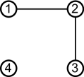
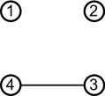
A closed-form expression for the limiting mean of the nodes states, i.e., the vector , and its correlation matrix , is also provided in Lemma 1 in Section 3.1. We refrain from stating them here as the expressions require significant amount of terminology to be introduced. The ergodic property of the Markov chain assumed in Theorem 2 ensures that the chain has a steady state distribution which is an entry-wise positive vector. Intuitively, ergodicity of the chain means that every graph in the set appears infinitely often as time progresses. In other words, the network does not get stuck in one of the graphs in the set . As a result, if a node is connected to the source in the union graph, even if it is not connected to the source in any one of the graphs that can ever appear, there is still a path for information flow between the source node and this node over time. Figure 3 shows a simple example in which the network can be only one of the two graphs shown in the figure. Node is disconnected from the source at every , but it is connected in a time-average sense since information from the source node can flow to in one time instant when the graph occurs and then from to in another time instant when occurs. In a such a situation the theorem guarantees that the expected value of the state of the node will converge to positive number. Thus, node can detect that it is connected to the source in a time-average sense. On the other hand, if a node is not connected to the source in the union graph there is no path for information flow between itself and the source over all time. This is equivalent to the node being permanently disconnected from the source, so the result that the mean of the node’s state converges to is consistent with the result of Theorem 1. The condition that is entry-wise positive means that there is a non-zero probability that the network at time can transition into any one of the possible graphs at time , even though most of these probabilities maybe small. We believe this sufficient condition is merely an artifact of our proof technique, and in fact, this is not a necessary condition for convergence to occur.
Remark 1.
An advantage of the DSSD algorithm is that its convergence rate for a time-invariant network is independent of the number of agents in the network (Lemma 1 in [8]). This makes the algorithm scalable to large networks. The convergence rate of mean and variance of the nodes states to their limiting values in the mobile case, however, requires further research.
3.1 Proof of Theorem 2
We start with some notation. let be the degree matrix of , i.e., . If node fails at , we assign and (the empty set) for . Let be the adjacency matrix of the graph , i.e., if , and otherwise. With these matrices, (1) can be compactly written as:
| (3) |
where . Recall that the source node has been indexed as node . The above can be written as
| (4) |
where the matrices and the vector are defined as
| (5) |
Under the assumption that the temporal evolution of the graphs is governed by a Markov chain, we can write (3) in the standard notation of jump-linear system [13]
| (6) |
where , , and . This notation is used to emphasize that the state and input matrices and of the linear system (6) change randomly, and the transition is governed by a Markov chain.
Let , be the mean and correlation of the state vector , respectively. We need the following definitions and terminology from [13] to provide expressions for these quantities as well as to state conditions for the convergence of the mean and correlation. Let be the space of real matrices. Let be the set of all N-sequences of real matrices . That is, if then , where each is an matrix. The operators and are defined as follows: let be the -th column of , then
| and | (13) |
Hence, and . Similarly, define an inverse function that produces an element of given a vector in . For for , define
| (17) |
For a set of square matrices , , we also use the notation to denote the following matrix:
In context of the jump linear system (6), define the matrices
| (18) |
where is the identity matrix, is the transition probability matrix of the Markov chain and denotes Kronecker product. Note that the matrices and can be expressed, using the notation introduced above, as
| (19) |
where is -th entry of and is the stationary distribution of the Markov chain, which exists due to the ergodicity directly followed by assumption of positive .
For a matrix , we write to mean that is entry-wise non-negative and write to mean and . If every entry of is positive, we write . For a matrix , means it is positive semi-definite (definite). For two matrices and of compatible dimension, we write if for all , , and write if and . For a vector , we write to mean is entry-wise non-negative, to mean is entry-wise non-negative and at least one entry is positive, and to mean every entry of is positive. The fact that both and are entry-wise non-negative will be useful later.
We will also need the following technical results to prove Theorem 2.
Proposition 1 ([14], Theorem 3.2).
Let be a block matrix, where are non-negative matrices for all and let , where is either the induced 1-norm () or the induced -norm ( ). Then .
Proposition 2.
Let be an undirected graph with nodes, and let , where and are the degree and adjacency matrices, respectively. and .
Proof.
Based on examining the structure of , we see that , where is if and otherwise. Obviously, is non-negative matrix and so is . Meanwhile, each row sum of is at most , where is the number of nodes. Therefore , which leads to , where the equality is a result of properties of the Kronecker product [15, Section 2.5]. ∎
Proposition 3.
If the temporal evolution of the graph is governed by a Markov chain that is ergodic, then we have and , where are defined in (3.1).
Proof.
Since (see (19)), we obtain by applying Proposition 1 that
where the equality follows from ’s being probabilities and therefore non-negative. Since (Proposition 2), it follows that . Since both and are non-negative, and is irreducible (which follows from the ergodic assumption of the Markov chain), it follows from Corollary 1.5 of [16, pg. 27] that , the last equality being a property of a transition probability matrix. This proves that .
To show that , since (see (19)), we obtain by applying Proposition 1 that
where the equality follows from ’s being probabilities and therefore non-negative. Since the scalars satisfy for each (see Proposition 2), it follows that . Since both and are non-negative, and is irreducible (which follows from the ergodic assumption of the Markov chain), it follows from Corollary 1.5 of [16, pg. 27] that , the last equality being a property of a transition probability matrix. This proves that . ∎
The proof of Theorem 2 will require the following result.
Lemma 1.
Consider the jump linear system (6) with the an underlying Markov chain that is ergodic. If , where is defined in (3.1), then the state of the system (6) converges in the mean square sense, i.e., and , where and are given by
| (20) |
where
where
| and | ||||||
| and |
and is defined in (3.1), is the -th entry of the steady state distribution of the Markov chain, and are the system matrices in (6). Moreover, .
Proof.
The first statement about mean square convergence follows from standard results in jump linear systems, as do the expressions for the mean and correlation; see [13, Proposition 3.37]. Note that the existence of the steady state distribution follows from the ergodicity of the Markov chain.
To show that is entry-wise non-negative, note that since (Proposition 3), we have . Thus, since is non-negative (which follows from the fact that and ’s). It follows from the expression for that it is also non-negative vector. This shows that , which implies . ∎
Now we are ready to prove Theorem 2
Proof of Theorem 2.
It follows from Proposition 3 that under the hypothesis of the Markov chain being ergodic, we have . It then follows from Lemma 1 that the state converges in the mean square sense, which proves the first statement of the theorem. Note that the limiting mean and correlation of the state is also provided by Lemma 1.
We already know from Lemma 1 that . To prove the last statement of the theorem, that if and only if there is a path between node and the source node in the union graph, we have to look at the structure of the tall vector in (20) more carefully, since completely determines . With some abuse of notation, from now on the source node will be referred to as node instead of . Note that which follows from ergodicity, by assumption, is a diagonal matrix with positive diagonal entries for every (follows from its definition), and , where and . It is easy to show now that the for some . Thus, . Since (Proposition 3), . Now, we express the matrix in terms of its blocks: , where are matrices. Then, can be rewritten as,
Therefore, , where the subscript denotes the first column of the corresponding matrix. Hence, the -th entry of is . Recall that . Therefore if and only if for , which is also equivalent to .
The subsequent discussion requires introducing directed graphs associated with matrices. For every matrix , define be the directed graph corresponding to as follows: the node set is the index set and the edge set is defined by if and only if [17]. It is a standard result in graph theory that the number of walks from a vertex to vertex in a directed graph of length is the -th element of , where is the adjacency matrix of the graph [18, pp. 165]. Since , it follows from the preceding discussion that the -th entry of is positive if and only if there exists a path from the vertex to vertex in the directed graph . Note that the graph contains nodes. We can group nodes into clusters such that each cluster, containing nodes, can be thought of as copies of the nodes in the sensor and robot network. To prevent confusion between the vertices in and node set of the original network, we use to denote a node in the graph that is the -th copy of the node in , where .
Therefore is equivalent to there being no directed path from any of the ’s copies () to any of ’s copies () in the directed graph . Otherwise, . Since existence of an edge from to in only depends on whether the -th entry of is non-zero, and does not depend on the specific value of the entry, it is convenient to define be a matrix associated with the matrix , such that if and if . Since , we have
It can be seen in a straightforward manner upon examining the matrix that if there is an edge between nodes and in the -th graph , i.e., , then for all , and for all , i.e., there are edges in from all copies of to , the -th copy of , and from all copies of to , the -th copy of .
Now we will show that if an arbitrary node is connected to in the union graph , then there is a path from a copy of to a copy of in the directed graph , otherwise not. To see that this is the case, we first take an example: consider a path of length from to in the union graph that involves two edges in two distinct graphs: and . From the preceding discussion, we have that , and . Thus a path from a copy of to a copy of in is . This argument works as long as there is a path from to in the union graph, irrespective of how long the path is. This shows that is connected to in the union graph, then there is a path from at least one of its copies to one of ’s copies in the directed graph , which means . If, however, is not connected to in the union graph, we can show that there is no path from any of ’s copies to any of ’s copies. This can be shown by considering the set of all nodes that do not have paths to in the union graph and the set of nodes that do separately; see [19] for details. This concludes the proof of the last statement of the theorem. ∎
4 Simulation Tests
The DSSD algorithm was tested in a simulation for a network consisting of agents initially deployed in a unit square at random. Two agents can only establish direct communication if their Euclidean distance is less than . The source strength and cut detection threshold was and , respectively. Since there is no existing prior work on the problem of detecting separation in mobile networks that can operate without multi-hop routing, we do not provide simulation comparison with existing algorithms. Note that the solutions proposed in [9, 10] require routing between the nodes and the base station, which is challenging in sensor and robotic networks in which the topology can change with time quickly.
4.1 Performance of DSSD in a static network
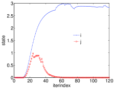
The first set of simulations is conducted with static nodes (see Figure 4(a)). The center node (symbolized by a triangle) is the source node. Simulations are run in a synchronous manner and a neighbor is removed from the list of neighbors of a node the first time it failed to receive messages from that neighbor. At the nodes shown as red squares in Figure 4(b) fail, leading to a cut in the network. Figure 4(c-d) show the time evolution of the states (calculated using (1)) of the four nodes , , , and . Node is the only one among the four that is separated from the source after the cut occurs. Initially, the states of every node increase from and then settle down to their steady state value. After the cut occurs, the state of node decreases towards . When the state of node decreases below the preset threshold , it declares itself cut from the source. This occurs at , thus the delay between the occurrence of the cut and its detection by is time-steps.
4.2 Performance of DSSD in a mobile network
Figures 5(a-d) show four snapshots of a communication network of mobile agents. The agents are divided into two groups, though there is no clear spatial separation between the two groups initially. The position of agent , denoted by , is updated according to:
| (21) |
where , , for every and , are independent random numbers. For agents in the first group, both and are normally distributed with mean and variance . For the second group, , are normally distributed with mean and variance . The motion of the agents results in the network composed of two disjoint components at , four components at , and then again two components at .
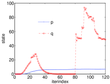
The evolution of the states of four agents , , , and are shown in Figure 6(a-b). The loss of connectivity of agent from the source occurs at and is detected at . Connectivity to the source is regained at and is detected at (when the states became greater than ).
These simulations provide evidence that the algorithm is indeed effective in detecting disconnections and re-connections, irrespective of whether the network is made up of static or mobile agents.
5 System Implementation and Experimental Evaluation
In this section we describe the implementation, deployment and performance evaluation of a separation detection system for robotic sensor networks based on the DSSD algorithm. We implemented the system, using the nesC language, on Berkeley motes [20] running the TinyOS operating system [21]. The code uses 16KB of program memory and 719B of RAM. The separation detection system executes in two phases: Reliable Neighbor Discovery, and the DSSD algorithm.
In the Reliable Neighbor Discovery Phase each node broadcasts a set of beacons in a small, fixed, time interval. Upon receiving a beacon from node , a node updates the number of beacons received from node . Next, an iteration of the DSSD algorithm executes. To determine whether a communication link is established, each node first computes for each of its neighbors the Packet Reception Ratio (PRR), defined as the ratio of the number of successfully received beacons received from, to the total number of beacons sent by, a neighbor. A neighbor is deemed reliable if the . After receiving state information from neighbors, a node updates its state according to Equation (1) and broadcasts its new state. When broadcast from a neighbor is not received for 2 iterations, the last reported state of the neighbor is used for calculating the state. A neighbor from which broadcast is not received for 4 iterations is permanently removed from the neighbor table. The state is stored in the 512KB on-board flash memory at each iteration (for a total of about 1.6KB for 200 iterations) for post-deployment analysis. In order to monitor connectivity information each node broadcasts its neighbor table along with the state.
To ensure a lock-step execution of the algorithm, all nodes are started at approximately the same time. For this, a mote acting as a base station, connected to a laptop, broadcasts a “system start” message, which is resent by each sensor node at most once. The base station is also used for monitoring the execution of the algorithm and monitoring the inter-mote communication.
5.1 Experimental Performance Evaluation in Static Network
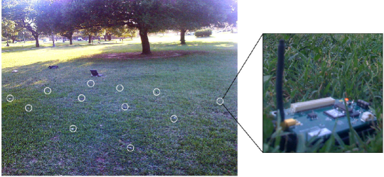
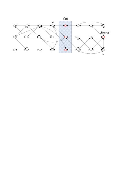
For evaluating the performance of our separation detection system in static networks, we deployed a network of 24 motes in a 135m2 outdoor field at Texas A&M University. Because the motes were positioned on the ground the radio range was reduced considerably with a one-hop distance of about 1.5m. The network connectivity is depicted in Figure 8(a). A partial view of the outdoor deployment is shown in Figure 7.
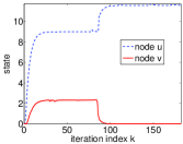
In our deployment, the source strength was specified as , the iteration length was 5sec (this value could be reduced easily to as small as msec) and the cut detection threshold was . Experimental results for two of the sensor nodes deployed are shown in Figure 8. After about 30 iterations the states of all nodes converged. At iteration a cut is created by turning off motes inside the rectangle labeled “Cut” in Figure 8(a). Figures 8(b) and 8(c) show the states for nodes and , as depicted in Figure 8(a), which were connected and disconnected, respectively, from the source node after the cut. The evolution of their states follows the aforementioned experimental scenario. Node declares itself cut from the source at , since its state falls below the threshold at that time.
5.2 Experimental Performance Evaluation in Mobile Network
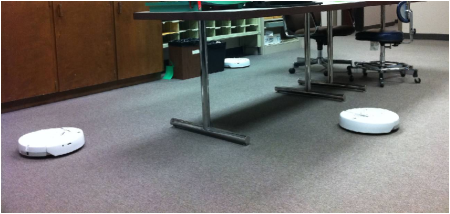
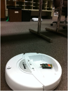
For evaluating the performance of our separation detection system in mobile networks we deployed 8 sensor nodes in an indoor environment, with 4 of the nodes residing on Roomba robots and 4 on human subjects. The scenario we emulated was that of a robotic-assisted emergency response team. Figure 9 shows part of the test set-up with the mobile nodes.
The network topologies as well as the locations of the nodes at a few time instants are shown in Figure 10. As we can see from the figure, the topology of the network varied greatly over time due to the mobility of the nodes.
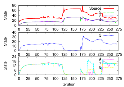
Figure 11 shows the time-traces of the node states during the experiment. The network is connected until time , and the states of all nodes converges to positive numbers; see Figure 11(a). This is consistent with the prediction of theorem 2. At approximately iteration , four of the nodes (nodes 5 through 8), carried by human subjects, are disconnected from the rest of the network, and in particular, from the source node . A sample network topology during the time interval to is shown in Figure 10(b). As we can see from Figure 11(b-c), the states of the disconnected nodes through converge to zero. The nodes detect that they are separated from the source, at times respectively, when their states become lower than the threshold . At approximately iteration , node joins back the sub-network formed by nodes -. As a result of node moving, node becomes a bridge between the two sub-networks. Hence, after iteration , the states of nodes , and become positive (hence, a fully connected network). However, this re-connection is temporary, and nodes through again become disconnected from the source after some time, which is seen in their states. Another temporary connection occurs between the set of nodes - and the set of nodes -, during the time interval through , followed by a separation. Finally, after iteration , the network becomes connected again, as shown in Figure 10(d). As a result, the states of all the nodes become positive after time , and they detect their re-connections to the source.
6 Conclusions
In this paper we introduced the Distributed Source Separation Detection (DSSD) algorithm to detect network separation in robotic and sensor networks. Simulations and hardware experiments demonstrated the efficacy of the algorithm. DSSD requires communication only between neighbors, which avoids the need for routing, making it particularly suitable for mobile networks. The algorithm is distributed, doesn’t require time synchronization among nodes, and the computations involved are simple. The DSSD algorithm is applicable to a heterogeneous network of static as well as mobile nodes, with varying levels of resources, precisely the kind envisioned for robotic and sensor networks.
References
- McKee and Schenker [2003] G. McKee, P. Schenker, Proceedings of SPIE 4196 (2003) 197.
- Hsieh et al. [2007] M. A. Hsieh, L. Chaimowicz, A. Cowley, B. Grocholsky, J. Keller, V. Kumar, C. J. Taylor, Y. Endo, R. Arkin, B. Jung, D. F. Wolf, G. S. Sukhatme, D. MacKenzie, Journal of Field Robotics 24 (2007) 991–1014.
- Kumar et al. [2004] V. Kumar, D. Rus, S. Singh, IEEE Pervasive Computing 3 (2004) 24–33.
- Perkins et al. [2003] C. Perkins, E. Belding-Royer, S. Das, in: IETF RFC, RFC Editor, United States, 2003.
- Juang et al. [2002] P. Juang, H. Oki, Y. Wang, M. Martonosi, L. S. Peh, D. Rubenstein, in: Tenth International Conference on Architectural Support for Programming Languages and Operating Systems(ASPLOS-X).
- Shrivastava et al. [2008] N. Shrivastava, S. Suri, C. D. Tóth, ACM Trans. Sen. Netw. 4 (2008) 1–25.
- Kleinberg [2003] J. Kleinberg, Internet Mathematics 1 (2003) 37–56.
- Barooah [2008] P. Barooah, in: 47th IEEE Conference on Decision and Control, pp. 1097 – 1102.
- Hauspie et al. [2003] M. Hauspie, J. Carle, D. Simplot, in: 2nd Mediterranean Workshop on Ad-Hoc Networks, pp. 25–27.
- Ritter et al. [2004] H. Ritter, R. Winter, J. Schiller, T. Zippan, in: NetGames ’04: Proceedings of 3rd ACM SIGCOMM workshop on Network and system support for games, ACM, New York, NY, USA, 2004, pp. 169–169.
- Hsieh et al. [2007] M. A. Hsieh, A. Cowley, V. Kumar, C. J. Taylor, Journal of Robotic Systems 25 (2007) 111 – 131. Special Issue on Search and Rescue Robots.
- Diestel [2000] R. Diestel, Graph theory, Springer New York, 2000.
- Costa et al. [2004] O. Costa, M. Fragoso, R. Marques, Discrete-Time Markov Jump Linear Systems, Probability and its Applications, Springer, 2004.
- Chen and Li [2004] M.-Q. Chen, X. Li, Linear Algebra and its Applications (2004).
- Langville and Stewart [2004] A. N. Langville, W. J. Stewart, Journal of Computational and Applied Mathematics 167 (2004) 429–447.
- Berman and Plemmons [1979] A. Berman, R. J. Plemmons, Nonnegative Matrices in the Mathematical Sciences, Computer Science and Applied Mathematics, Academic Press, 1979.
- Meyer [2001] C. D. Meyer, Matrix Analysis and Applied Linear Algebra, SIAM: Society for Industrial and Applied Mathematics, 2001.
- Godsil and Royle [2001] C. Godsil, G. Royle, Algebraic Graph Theory, Graduate Texts in Mathematics, Springer, 2001.
- Liao et al. [2011] C. Liao, H. Chenji, P. Barooah, R. Stoleru, T. Kalmár-Nagy, Detecting Separation in Robotic and Sensor Networks, Technical Report, University of Florida, 2011. Http://plaza.ufl.edu/cdliao/.
- Inc. [2004] C. Inc., http://www.xbow.com/Products/Product_pdf_files/Wireless_pdf/MICAZ_Datasheet.pdf, 2004.
- Hill et al. [2000] J. Hill, R. Szewczyk, A. Woo, S. Hollar, D. Culler, K. Pister, in: ASPLOS-IX: Proceedings of the ninth international conference on Architectural support for programming languages and operating systems, volume 34, ACM Press, 2000, pp. 93–104.