Selecting the rank of truncated SVD
by Maximum Approximation Capacity

Mario Frank and Joachim M. Buhmann mario.frank@inf.ethz.ch, jbuhmann@inf.ethz.ch Department of Computer Science, ETH Zurich; Universit tsstrasse 6, CH-8006 Z rich, Switzerland
Abstract

Truncated Singular Value Decomposition (SVD) calculates the closest rank-k๐‘˜k approximation of a given input matrix. Selecting the appropriate rank k๐‘˜k defines a critical model order choice in most applications of SVD. To obtain a principled cut-off criterion for the spectrum, we convert the underlying optimization problem into a noisy channel coding problem. The optimal approximation capacity of this channel controls the appropriate strength of regularization to suppress noise. In simulation experiments, this information theoretic method to determine the optimal rank competes with state-of-the art model selection techniques.

I Introduction

Singular Value Decomposition (SVD) is a widely used technique for exploratory data analysis. It decomposes a given input matrix into a product of three matrices such that ๐—=๐”๐’๐•T๐—superscript๐”๐’๐•๐‘‡\mathbf{X}=\mathbf{U}\mathbf{S}\mathbf{V}^{T}. Thereby, ๐”๐”\mathbf{U} and ๐•๐•\mathbf{V} are unitary matrices and they essentially induce a rotation of the input data. ๐’๐’\mathbf{S} is a diagonal matrix (inducing a scaling) with the singular values as entries. Quite often, one is rather interested in an approximation of ๐—๐—\mathbf{X} instead of the exact decomposition such as, for instance, in Principal Components Analysis (PCA). For SVD, this approximation technically requires to set all but the first k๐‘˜k diagonal entries in ๐’๐’\mathbf{S} to 00. The resulting reconstruction ๐”๐’kโ€‹๐•Tsubscript๐”๐’๐‘˜superscript๐•๐‘‡\mathbf{U}\mathbf{S}_{k}\mathbf{V}^{T} has rank k๐‘˜k. Neglecting all but the first k๐‘˜k components is justified since the noise in the data perturbs the small eigenvalues, whereas the first k๐‘˜k components supposedly capture the underlying structure or the signal of the data. Selecting the cutoff value k๐‘˜k defines the central model-order selection problem of truncated SVD.

In this paper we propose a novel method for selecting k๐‘˜k which is based on the framework of approximation set coding (ASC) [1]. ASC defines the maximum approximation capacity (maxAC) principle for model-order selection. For a given model order and a given noisy dataset, ASC theory enables us to compute the capacity of a hypothetical channel. MaxAC selects the model that achieves highest capacity, i.e., the model of highest complexity that still can be robustly optimized in the presence of noise. Originally, maxAC was derived for discrete optimization problems. So far, it was applied to decoding for the binary channel [1] and for selecting the number of clusters in clustering problems [2]. In this contribution, we adopt it, for the first time, to a continuous optimization problem, namely for selecting the cut-off rank of truncated SVD. Thereby, we investigate the challenges of the continuous solution space. Moreover, we provide an experimental comparison with other model-selection methods indicating that our maxAC adaption to SVD can compete with state-of-the art methods. In the remainder of the paper we will first introduce the main concepts of ASC in Sectionย II. In Sectionย III we then derive the approximation capacity for SVD, point to problems and solutions and report our numerical findings.

II Approximation Set Coding

In this section we briefly recapitulate the principle of maximum approximation capacity (maxAC). Due to the page limit, we must refer to the original paper [1] for a more detailed description.

Consider a generic optimization problem with the input ๐—={๐ฑ1,โ€ฆ,๐ฑN}โˆˆ๐’ณ๐—subscript๐ฑ1โ€ฆsubscript๐ฑ๐‘๐’ณ\mathbf{X}=\{\mathbf{x}_{1},\dots,\mathbf{x}_{N}\}\in\mathcal{X} consisting out of N๐‘N measurements. The vector ๐ฑiโˆˆโ„Dsubscript๐ฑ๐‘–superscriptโ„๐ท\mathbf{x}_{i}\in\mathbb{R}^{D} identifies the ithsuperscript๐‘–thi^{\textrm{th}} measurement. Let the output of the optimization problem be the solution or hypothesis cโˆˆ๐’ž๐‘๐’žc\in\mathcal{C} where ๐’ž๐’ž\mathcal{C} is the set of all hypotheses satisfying the constraints of the problem, the hypothesis space. An optimization problem involves a cost function R:๐’žร—๐’ณโ†’โ„โ‰ฅ0:๐‘…โ†’๐’ž๐’ณsubscriptโ„absent0R\,:\,\mathcal{C}\times\mathcal{X}\rightarrow\mathbb{R}_{\geq 0} that maps a hypothesis c๐‘c to a real value Rโ€‹(c,๐—)๐‘…๐‘๐—R(c,\mathbf{X}). Finally, let cโŠฅ=argโกmincโกRโ€‹(c,๐—)superscript๐‘bottomsubscript๐‘๐‘…๐‘๐—c^{\bot}=\arg\min_{c}R(c,\mathbf{X}) be the hypothesis that minimizes costs. In order to rank all solutions of the optimizer, we introduce approximation weights

w:๐’žร—๐’ณร—โ„+:๐‘ค๐’ž๐’ณsubscriptโ„\displaystyle w:\mathcal{C}\times\mathcal{X}\times\mathbb{R}_{+} โ†’โ†’\displaystyle\rightarrow [0,1],01\displaystyle[0,1]\,, (1)
(c,๐—,ฮฒ)๐‘๐—๐›ฝ\displaystyle(c,\mathbf{X},\beta) โ†ฆmaps-to\displaystyle\mapsto wฮฒโ€‹(c,๐—)=expโก(โˆ’ฮฒโ€‹Rโ€‹(c,๐—)).subscript๐‘ค๐›ฝ๐‘๐—๐›ฝ๐‘…๐‘๐—\displaystyle w_{\beta}(c,\mathbf{X})=\exp(-\beta R(c,\mathbf{X}))\,.

These weights, parameterized by the inverse computational temperature ฮฒ๐›ฝ\beta, define the two weight sums ๐’ต1,๐’ต2subscript๐’ต1subscript๐’ต2\mathcal{Z}_{1},\mathcal{Z}_{2}, and the joint weight sum ๐’ต12subscript๐’ต12\mathcal{Z}_{12}

๐’ตฮฝsubscript๐’ต๐œˆ\displaystyle\mathcal{Z}_{\nu} :=assign\displaystyle:= โˆ‘cโˆˆ๐’žexpโก(โˆ’ฮฒโ€‹Rโ€‹(c,๐—(ฮฝ))),ฮฝ=1,2formulae-sequencesubscript๐‘๐’ž๐›ฝ๐‘…๐‘superscript๐—๐œˆ๐œˆ12\displaystyle\sum_{c\in\mathcal{C}}\exp\left(-\beta R(c,\mathbf{X}^{(\nu)})\right),\>\nu=1,2 (2)
๐’ต12subscript๐’ต12\displaystyle\mathcal{Z}_{12} :=assign\displaystyle:= โˆ‘cโˆˆ๐’žexpโก(โˆ’ฮฒโ€‹(Rโ€‹(c,๐—(1))+Rโ€‹(c,๐—(2)))),subscript๐‘๐’ž๐›ฝ๐‘…๐‘superscript๐—1๐‘…๐‘superscript๐—2\displaystyle\sum_{c\in\mathcal{C}}\exp\left(-\beta(R(c,\mathbf{X}^{(1)})+R(c,\mathbf{X}^{(2)}))\right), (3)

where ๐—(1)superscript๐—1\mathbf{X}^{(1)} and ๐—(2)superscript๐—2\mathbf{X}^{(2)} are two random subsets of the input ๐—๐—\mathbf{X} and expโก(โˆ’ฮฒโ€‹(Rโ€‹(c,๐—(1))+Rโ€‹(c,๐—(2))))๐›ฝ๐‘…๐‘superscript๐—1๐‘…๐‘superscript๐—2\exp(-\beta(R(c,\mathbf{X}^{(1)})+R(c,\mathbf{X}^{(2)}))) measures how well a single solution c๐‘c minimizes costs on both datasets. The sums (2,3) play a central role in ASC. If ฮฒ=0๐›ฝ0\beta=0, all weights wฮฒโ€‹(c,๐—)=1subscript๐‘ค๐›ฝ๐‘๐—1w_{\beta}(c,\mathbf{X})=1 are independent of the costs. In this case, ๐’ตฮฝ=|๐’ž|subscript๐’ต๐œˆ๐’ž\mathcal{Z}_{\nu}=|\mathcal{C}| indicates the size of the hypothesis space, and ๐’ต12=๐’ต1=๐’ต2subscript๐’ต12subscript๐’ต1subscript๐’ต2\mathcal{Z}_{12}=\mathcal{Z}_{1}=\mathcal{Z}_{2}. For intermediate ฮฒ๐›ฝ\beta, ๐’ตโ€‹(โ‹…)๐’ตโ‹…\mathcal{Z}(\cdot) takes a value between 00 and |๐’ž|๐’ž|\mathcal{C}|, giving rise to the interpretation of ๐’ตโ€‹(โ‹…)๐’ตโ‹…\mathcal{Z}(\cdot) as the effective number of hypotheses that approximately fit the dataset ๐—(ฮฝ)superscript๐—๐œˆ\mathbf{X}^{(\nu)}, whereas ฮฒ๐›ฝ\beta defines the precision of this approximation.

ASC constructs a hypothetical coding scenario where sender and receiver have to communicate problem solutions via transformations ฯ„โˆˆ๐’ฏ๐œ๐’ฏ\tau\in\mathcal{T} of noisy datasets ๐—(1)superscript๐—1\mathbf{X}^{(1)} and ๐—(2)superscript๐—2\mathbf{X}^{(2)}. As derived in [1], an asymptotically vanishing error rate for such a channel is achievable for rates

ฯ๐œŒ\displaystyle\rho โ‰ค\displaystyle\leq โ„ฮฒโ€‹(ฯ„s,ฯ„^)=1Nโ€‹logโก(|{ฯ„s}|โ‹…๐’ต12๐’ต1โ‹…๐’ต2).subscriptโ„๐›ฝsubscript๐œ๐‘ ^๐œ1๐‘โ‹…subscript๐œ๐‘ subscript๐’ต12โ‹…subscript๐’ต1subscript๐’ต2\displaystyle\mathcal{I}_{\beta}(\tau_{s},\hat{\tau})={\frac{1}{N}}\log\left(\frac{|\{\tau_{s}\}|\cdot\mathcal{Z}_{12}}{\mathcal{Z}_{1}\cdot\mathcal{Z}_{2}}\right)\ . (4)

Eq.(4) denotes the mutual information between the encoded transformation ฯ„ssubscript๐œ๐‘ \tau_{s} of the dataset and the decoded transformation ฯ„^^๐œ\hat{\tau}. A higher approximation precision ฮฒ๐›ฝ\beta has two effects. First, the hypothesis space is covered by more patches of approximate solutions leading to more available codewords and a higher codeword entropy |{ฯ„s}|subscript๐œ๐‘ |\{\tau_{s}\}|. Second, these patches have a higher overlap such that, in the decoding step, codewords are possibly confused. The maximum of โ„ฮฒโ€‹(ฯ„s,ฯ„^)subscriptโ„๐›ฝsubscript๐œ๐‘ ^๐œ\mathcal{I}_{\beta}(\tau_{s},\hat{\tau}) with respect to ฮฒ๐›ฝ\beta is called the approximation capacity.

III Approximation capacity of SVD

To select the cut-off rank for SVD, we have to find the rank kโˆ—superscript๐‘˜k^{*} with maximal approximation capacity. This search involves maximizing Eq.(4) for all ranks that we investigate. By going through the list of all quantities introduced in the last section, we relate them to truncated SVD. The input of the problem is a matrix ๐—โˆˆโ„Nร—D๐—superscriptโ„๐‘๐ท\mathbf{X}\in\mathbb{R}^{N\times D}. The cost function is the Frobenius norm:

Rโ€‹(๐—,๐”,๐’,๐•)=โˆ‘i,j(xiโ€‹jโˆ’โˆ‘t=1kuiโ€‹tโ€‹stโ€‹tโ€‹vtโ€‹j)2๐‘…๐—๐”๐’๐•subscript๐‘–๐‘—superscriptsubscript๐‘ฅ๐‘–๐‘—superscriptsubscript๐‘ก1๐‘˜subscript๐‘ข๐‘–๐‘กsubscript๐‘ ๐‘ก๐‘กsubscript๐‘ฃ๐‘ก๐‘—2R(\mathbf{X},\mathbf{U},\mathbf{S},\mathbf{V})=\sum_{i,j}\left(x_{ij}-\sum_{t=1}^{k}u_{it}s_{tt}v_{tj}\right)^{2} (5)

An optimizer for this problem outputs a decomposition cโŠฅโ€‹(๐—(ฮฝ))=๐”(ฮฝ)โ€‹๐’(ฮฝ)โ€‹๐•(ฮฝ)superscript๐‘bottomsuperscript๐—๐œˆsuperscript๐”๐œˆsuperscript๐’๐œˆsuperscript๐•๐œˆc^{\bot}(\mathbf{X}^{(\nu)})=\mathbf{U}^{(\nu)}\mathbf{S}^{(\nu)}\mathbf{V}^{(\nu)}, whereas all but the first kโ‰คminโก(N,D)๐‘˜๐‘๐ทk\leq\min(N,D) diagonal entries of ๐’(ฮฝ)superscript๐’๐œˆ\mathbf{S}^{(\nu)} are 00 due to truncation (we will denote the third matrix by ๐•๐•\mathbf{V} instead of ๐•Tsuperscript๐•๐‘‡\mathbf{V}^{T} for convenience). The solution cโŠฅโ€‹(๐—(ฮฝ))superscript๐‘bottomsuperscript๐—๐œˆc^{\bot}(\mathbf{X}^{(\nu)}) gives the closest rank-k๐‘˜k approximation of ๐—(ฮฝ)superscript๐—๐œˆ\mathbf{X}^{(\nu)} with respect to the Frobenius norm. In the case of SVD, a hypothesis c=(๐”,๐’,๐•)๐‘๐”๐’๐•c=(\mathbf{U},\mathbf{S},\mathbf{V}) is a particular decomposition of the input matrix (in clustering, for instance, c๐‘c is a relation that assigns objects to clusters [2]). The kร—D๐‘˜๐ทk\times D matrix with the entries wtโ€‹j:=stโ€‹tโ€‹vtโ€‹jassignsubscript๐‘ค๐‘ก๐‘—subscript๐‘ ๐‘ก๐‘กsubscript๐‘ฃ๐‘ก๐‘—w_{tj}:=s_{tt}v_{tj} is a new basis and ๐”๐”\mathbf{U} provides the linear weights needed to represent the data ๐—๐—\mathbf{X} in this basis. When the empirical mean of ๐—๐—\mathbf{X} is the origin, this representation corresponds to PCA.

We define the hypothesis space for truncated SVD with cut-off rank k๐‘˜k as follows. For a fixed basis ๐–๐–\mathbf{W}, the hypothesis space is spanned by all Nร—k๐‘๐‘˜N\times k matrices ๐”๐”\mathbf{U}. For a given dataset ๐—(ฮฝ)superscript๐—๐œˆ\mathbf{X}^{(\nu)}, ๐”(ฮฝ)superscript๐”๐œˆ\mathbf{U}^{(\nu)} is the cost-minimizing solution. We parameterize the different transformations ฯ„โˆˆ๐’ฏ๐œ๐’ฏ\tau\in\mathcal{T} for encoding messages in datasets by ฯ„โˆ˜๐—(ฮฝ)=๐—(ฮฝ)+๐”ฯ„โ€‹๐–(ฮฝ)๐œsuperscript๐—๐œˆsuperscript๐—๐œˆsubscript๐”๐œsuperscript๐–๐œˆ\tau\circ\mathbf{X}^{(\nu)}=\mathbf{X}^{(\nu)}+\mathbf{U}_{\tau}\mathbf{W}^{(\nu)}. The identity transformation is ๐”id=0subscript๐”id0\mathbf{U}_{\text{id}}=0.

The mutual information Eq.ย (4) was originally derived for finite hypothesis spaces, such as for clustering solutions or binary message strings. The challenges of computing the weight sums (2) and (3) are twofold. First, in a small volume of a continuous hypothesis space, there are infinitely many transformations. Second, transformations can have infinite distance to each other such that the receiver can always distinguish an infinite subset of ๐’ฏ๐’ฏ\mathcal{T} even when the datasets are noisy. This makes the union bound in the derivation of the error-probability in [1], Eq.ย (7) inadequate. For these reasons, calculating the capacity under the assumption that ๐”๐”\mathbf{U} can be any real Nร—k๐‘๐‘˜N\times k matrix fails. In the following, we will first demonstrate the effect of this assumption by providing the naรฏve analytical calculation of the mutual information in Eq.ย (4). Then we introduce constraints on the transformations ๐’ฏ๐’ฏ\mathcal{T} such that Eq.ย (4) can be computed.

III-A Unconstraint Hypothesis Space

We abbreviate Rฮฝ=Rโ€‹(๐—(ฮฝ),๐”,๐’(ฮฝ),๐•(ฮฝ))subscript๐‘…๐œˆ๐‘…superscript๐—๐œˆ๐”superscript๐’๐œˆsuperscript๐•๐œˆR_{\nu}=R(\mathbf{X}^{(\nu)},\mathbf{U},\mathbf{S}^{(\nu)},\mathbf{V}^{(\nu)}) and Rฮ”=1/2โ€‹(Rโ€‹(๐—(1),๐”,๐’(1),๐•(1))+Rโ€‹(๐—(2),๐”,๐’(1),๐•(1)))subscript๐‘…ฮ”12๐‘…superscript๐—1๐”superscript๐’1superscript๐•1๐‘…superscript๐—2๐”superscript๐’1superscript๐•1R_{\Delta}=1/2\left(R(\mathbf{X}^{(1)},\mathbf{U},\mathbf{S}^{(1)},\mathbf{V}^{(1)})+R(\mathbf{X}^{(2)},\mathbf{U},\mathbf{S}^{(1)},\mathbf{V}^{(1)})\right) and use the short-hand notation of ๐ฆ๐ข,.\mathbf{m_{i,.}} as the ithsuperscript๐‘–thi^{\text{th}} row of a matrix ๐Œ๐Œ\mathbf{M}. By integrating over the space of all linear combinations ๐”๐”\mathbf{U}, we obtain the weight sums:

๐’ตฮฝ=โˆซโˆ’โˆžโˆžexpโก[โˆ’ฮฒโ€‹Rฮฝ]โ€‹๐‘‘๐”,ฮฝโˆˆ{1,2}formulae-sequencesubscript๐’ต๐œˆsuperscriptsubscript๐›ฝsubscript๐‘…๐œˆdifferential-d๐”๐œˆ12\displaystyle\mathcal{Z}_{\nu}\!=\!\!\int_{-\infty}^{\infty}\!\!\!\exp\left[-\beta R_{\nu}\right]{d\mathbf{U}}\ ,\ \ \nu\in\left\{1,2\right\} (6)
=โˆiโ€‹jeโˆ’ฮฒโ€‹xiโ€‹j(ฮฝ)2โ€‹โˆซโˆ’โˆžโˆžeโˆ’ฮฒโ€‹((โˆ‘tkuiโ€‹tโ€‹wtโ€‹j(ฮฝ))2โˆ’2โ€‹xiโ€‹j(ฮฝ)โ€‹โˆ‘tkuiโ€‹tโ€‹wtโ€‹j(ฮฝ))โ€‹dkโ€‹๐ฎ๐ข,.\displaystyle=\prod_{ij}e^{-\beta{x_{ij}^{(\nu)}}^{2}}\!\!\int_{-\infty}^{\infty}\!\!\!e^{-\beta\left(\left(\sum_{t}^{k}u_{it}w_{tj}^{(\nu)}\right)^{2}-2x_{ij}^{(\nu)}\sum_{t}^{k}u_{it}w_{tj}^{(\nu)}\right)}{d^{k}\mathbf{u_{i,.}}}
๐’ต12=โˆซโˆ’โˆžโˆžexpโก[โˆ’ฮฒโ€‹Rฮ”]โ€‹๐‘‘๐”=โˆiโ€‹jeโˆ’ฮฒ/2โ€‹(xiโ€‹j(1)2+xiโ€‹j(2)2)subscript๐’ต12superscriptsubscript๐›ฝsubscript๐‘…ฮ”differential-d๐”subscriptproduct๐‘–๐‘—superscript๐‘’๐›ฝ2superscriptsuperscriptsubscript๐‘ฅ๐‘–๐‘—12superscriptsuperscriptsubscript๐‘ฅ๐‘–๐‘—22\displaystyle\mathcal{Z}_{12}\!=\!\!\int_{-\infty}^{\infty}\!\!\!\exp\left[-\beta R_{\Delta}\right]{d\mathbf{U}}=\prod_{ij}e^{-\beta/2\left({x_{ij}^{(1)}}^{2}+{x_{ij}^{(2)}}^{2}\right)} (7)
โ‹…โˆซโˆ’โˆžโˆžeโˆ’ฮฒ/2โ€‹(2โ€‹(โˆ‘tkuiโ€‹tโ€‹wtโ€‹j(1))2โˆ’2โ€‹(xiโ€‹j(1)+xiโ€‹j(2))โ€‹โˆ‘tkuiโ€‹tโ€‹wtโ€‹j(1))dk๐ฎ๐ข,.\displaystyle\cdot\!\!\int_{-\infty}^{\infty}\!\!\!e^{-\beta/2\left(2\left(\sum_{t}^{k}u_{it}w_{tj}^{(1)}\right)^{2}-2\left(x_{ij}^{(1)}+x_{ij}^{(2)}\right)\sum_{t}^{k}u_{it}w_{tj}^{(1)}\right)}{d^{k}\mathbf{u_{i,.}}}

The solution of Gaussian integrals yields

โˆซโˆ’โˆžโˆžeโˆ’1/2โ€‹โˆ‘tkโˆ‘tโ€ฒkAt,tโ€ฒโ€‹utโ€‹utโ€ฒ+โˆ‘tkbtโ€‹utsuperscriptsubscriptsuperscript๐‘’12superscriptsubscript๐‘ก๐‘˜superscriptsubscriptsuperscript๐‘กโ€ฒ๐‘˜subscript๐ด๐‘กsuperscript๐‘กโ€ฒsubscript๐‘ข๐‘กsubscript๐‘ขsuperscript๐‘กโ€ฒsuperscriptsubscript๐‘ก๐‘˜subscript๐‘๐‘กsubscript๐‘ข๐‘ก\displaystyle\!\!\int_{-\infty}^{\infty}\!\!\!e^{-1/2\sum_{t}^{k}\sum_{t^{\prime}}^{k}A_{t,t^{\prime}}u_{t}u_{t^{\prime}}+\sum_{t}^{k}b_{t}u_{t}}\!\! =\displaystyle\!\!=\!\! (2โ€‹ฯ€)kdet(๐€)โ€‹e1/2โ€‹๐›Tโ€‹๐€โˆ’1โ€‹๐›,superscript2๐œ‹๐‘˜๐€superscript๐‘’12superscript๐›๐‘‡superscript๐€1๐›\displaystyle\!\!\!\!\sqrt{\frac{\left(2\pi\right)^{k}}{\det(\mathbf{A})}}e^{1/2\mathbf{b}^{T}\mathbf{A}^{-1}\mathbf{b}}\ ,

whereas in our case

๐€(๐ฃ)(ฮฝ)=2โ€‹ฮฒโ€‹๐ฐ.,๐ฃ(ฮฝ)Tโ€‹๐ฐ.,๐ฃ(ฮฝ),๐›(๐ฃ)(ฮฝ)=2โ€‹ฮฒโ€‹xiโ€‹j(ฮฝ)โ€‹๐ฐ.,๐ฃ(ฮฝ)T,\displaystyle\mathbf{A^{(\nu)}_{(j)}}\!\!=\!\!2\beta\;\mathbf{w_{.,j}^{(\nu)}}^{T}\mathbf{w_{.,j}^{(\nu)}}\ ,\quad\ \mathbf{b^{(\nu)}_{(j)}}\!\!=\!\!2\beta\;x_{ij}^{(\nu)}\mathbf{w_{.,j}^{(\nu)}}^{T}\ , (8)
๐€(๐ฃ)(๐šซ)=๐€(๐ฃ)(๐Ÿ),๐›(๐ฃ)(๐šซ)=ฮฒโ€‹(xiโ€‹j(1)+xiโ€‹j(2))โ€‹๐ฐ.,๐ฃ(๐Ÿ)T.\displaystyle\mathbf{A^{(\Delta)}_{(j)}}\!\!=\!\!\mathbf{A^{(1)}_{(j)}}\ ,\quad\quad\quad\quad\quad\mathbf{b^{(\Delta)}_{(j)}}\!\!=\!\!\beta\left(x_{ij}^{(1)}+x_{ij}^{(2)}\right)\mathbf{w_{.,j}^{(1)}}^{T}\ .

The weight sums are

๐’ตฮฝ=โˆi,jeโˆ’ฮฒโ€‹xiโ€‹j(ฮฝ)โ€‹2โ€‹(2โ€‹ฯ€)kdet(2โ€‹ฮฒโ€‹๐ฐ.,๐ฃ(ฮฝ)Tโ€‹๐ฐ.,๐ฃ(ฮฝ))โ€‹e1/2โ€‹๐›Tโ€‹๐€โˆ’1โ€‹๐›\displaystyle\mathcal{Z}_{\nu}\!\!=\!\!\prod_{i,j}e^{-\beta x_{ij}^{(\nu)2}}\!\!\sqrt{\frac{(2\pi)^{k}}{\det\left(2\beta\;\mathbf{w_{.,j}^{(\nu)}}^{T}\mathbf{w_{.,j}^{(\nu)}}\right)}}e^{1/2\mathbf{b}^{T}\mathbf{A}^{-1}\mathbf{b}}
=(i)(ฯ€ฮฒ)Nโ€‹Dโ€‹k2โ€‹โˆj(Dj(ฮฝ))โˆ’N2โ€‹eโˆ’ฮฒโ€‹โˆ‘iโ€‹j(xiโ€‹j(ฮฝ)โ€‹2โ€‹(1โˆ’๐ฐ.,๐ฃ(ฮฝ)Tโ€‹(๐ฐ.,๐ฃ(ฮฝ)โ€‹๐ฐ.,๐ฃ(ฮฝ)T)โˆ’1โ€‹๐ฐ.,๐ฃ(ฮฝ)))\displaystyle\stackrel{{\scriptstyle(i)}}{{=}}\!\!\left(\frac{\pi}{\beta}\right)^{\!\!\frac{NDk}{2}}\!\!\!\!\!\!\prod_{j}\!\!\left(\!D^{(\nu)}_{j}\!\right)^{\,\frac{\!-N}{2}}\!\!e^{\!-\beta\sum_{\!ij}\left(x_{ij}^{(\nu)2}\left(1-\mathbf{w_{.,j}^{(\nu)}}^{T}(\mathbf{w_{.,j}^{(\nu)}}\mathbf{w_{.,j}^{(\nu)}}^{T})^{-1}\mathbf{w_{.,j}^{(\nu)}}\right)\right)}
=(iโ€‹i)(ฯ€ฮฒ)Nโ€‹Dโ€‹k2โ€‹โˆj(Dj(ฮฝ))โˆ’N2superscript๐‘–๐‘–absentsuperscript๐œ‹๐›ฝ๐‘๐ท๐‘˜2subscriptproduct๐‘—superscriptsubscriptsuperscript๐ท๐œˆ๐‘—๐‘2\displaystyle\stackrel{{\scriptstyle(ii)}}{{=}}\!\!\left(\frac{\pi}{\beta}\right)^{\frac{NDk}{2}}\prod_{j}\left(D^{(\nu)}_{j}\right)^{\,\frac{-N}{2}} (9)
๐’ต12=|Cฮณ(1)|โ€‹โˆiโ€‹jeโˆ’ฮฒ/4โ€‹(xiโ€‹j(1)โˆ’xiโ€‹j(2))2.subscript๐’ต12subscriptsuperscript๐ถ1๐›พsubscriptproduct๐‘–๐‘—superscript๐‘’๐›ฝ4superscriptsuperscriptsubscript๐‘ฅ๐‘–๐‘—1superscriptsubscript๐‘ฅ๐‘–๐‘—22\displaystyle\mathcal{Z}_{12}=\left|C^{(1)}_{\gamma}\right|\prod_{ij}e^{-\beta/4\left(x_{ij}^{(1)}-x_{ij}^{(2)}\right)^{2}}\ . (10)

We abbreviated Dj(ฮฝ):=det(๐ฐ.,๐ฃ(ฮฝ)โ€‹๐“โ€‹๐ฐ.,๐ฃ(ฮฝ))D^{(\nu)}_{j}:=\det(\mathbf{w_{.,j}^{(\nu)T}}\mathbf{w_{.,j}^{(\nu)}}). In step (i), we used that for a nร—n๐‘›๐‘›n\times n matrix ๐Œ๐Œ\mathbf{M} and a scalar p๐‘p, it holds that det(pโ€‹๐Œ)=pnโ€‹det(๐Œ)๐‘๐Œsuperscript๐‘๐‘›๐Œ\det\left(p\mathbf{M}\right)=p^{n}\det\left(\mathbf{M}\right). In step (ii), we used that ๐…(ฮฝ):=๐ฐ.,๐ฃ(ฮฝ)โ€‹(๐ฐ.,๐ฃ(ฮฝ)Tโ€‹๐ฐ.,๐ฃ(ฮฝ))โˆ’1โ€‹๐ฐ.,๐ฃ(ฮฝ)T=1\mathbf{F^{(\nu)}}:=\mathbf{w_{.,j}^{(\nu)}}(\mathbf{w_{.,j}^{(\nu)}}^{T}\mathbf{w_{.,j}^{(\nu)}})^{-1}\mathbf{w_{.,j}^{(\nu)}}^{T}=1. Substituting to Eq.ย (4) provides the mutual information:

Iโ€‹(ฮฒ)=1Nโ€‹(logโก(๐’ต12)โˆ’logโก(๐’ต1)โˆ’logโก(๐’ต2))๐ผ๐›ฝ1๐‘subscript๐’ต12subscript๐’ต1subscript๐’ต2\displaystyle I(\beta)\!=\frac{1}{N}\left(\log\left(\mathcal{Z}_{12}\right)-\log\left(\mathcal{Z}_{1}\right)-\log\left(\mathcal{Z}_{2}\right)\right) (11)
=Dโ€‹k2โ€‹logโก(ฮฒฯ€)+12โ€‹โˆ‘jDj(2)โˆ’ฮฒ4โ€‹Nโ€‹โˆ‘iโ€‹j(xiโ€‹j(1)โˆ’xiโ€‹j(2))2.absent๐ท๐‘˜2๐›ฝ๐œ‹12subscript๐‘—subscriptsuperscript๐ท2๐‘—๐›ฝ4๐‘subscript๐‘–๐‘—superscriptsuperscriptsubscript๐‘ฅ๐‘–๐‘—1superscriptsubscript๐‘ฅ๐‘–๐‘—22\displaystyle=\frac{Dk}{2}\log\left(\frac{\beta}{\pi}\right)+\!\!\frac{1}{2}\sum_{j}D^{(2)}_{j}\!\!-\frac{\beta}{4N}\sum_{ij}\left(x_{ij}^{(1)}-x_{ij}^{(2)}\right)^{2}\ .

The first order condition provides the optimal temperature

1/ฮฒโˆ—=12โ€‹Nโ€‹Dโ€‹kโ€‹โˆ‘iโ€‹j(xiโ€‹j(1)โˆ’xiโ€‹j(2))2.1superscript๐›ฝ12๐‘๐ท๐‘˜subscript๐‘–๐‘—superscriptsuperscriptsubscript๐‘ฅ๐‘–๐‘—1superscriptsubscript๐‘ฅ๐‘–๐‘—22\displaystyle 1/\beta^{*}=\frac{1}{2NDk}\sum_{ij}\left(x_{ij}^{(1)}-x_{ij}^{(2)}\right)^{2}\ . (12)

Note that the temperature monotonically increases with the distance of the two datasets, as one would expect: with more noise, the precision for approximating the optimal solution must be lower. However, unexpectedly, the temperature decreases with k๐‘˜k suggesting that a higher rank stabilizes the solutions. This misconception is a consequence of the unconstrained hypothesis space, as discussed earlier, and indicates that constraints for ๐”๐”\mathbf{U} are necessary. Also, we neglected the temperature-independent term |{ฯ„s}|subscript๐œ๐‘ |\{\tau_{s}\}| in Eq.ย (4) which would be infinitely high.
Refer to caption
Refer to caption
Refer to caption
Refer to caption
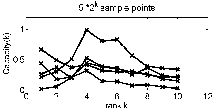
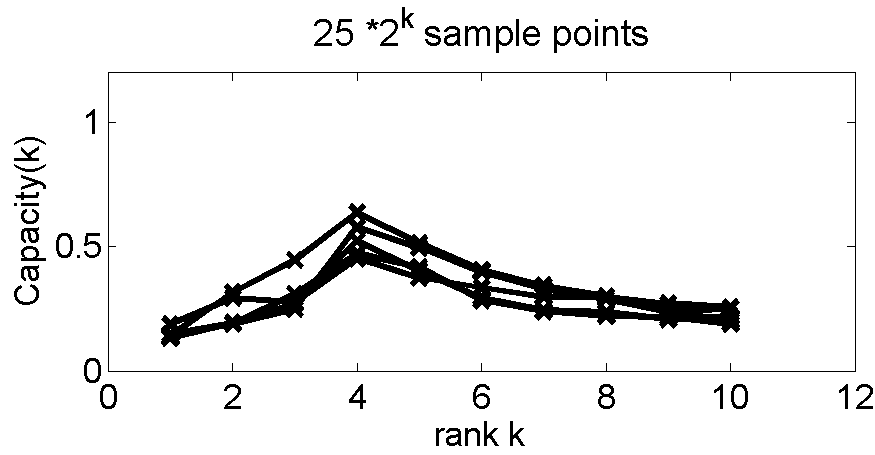
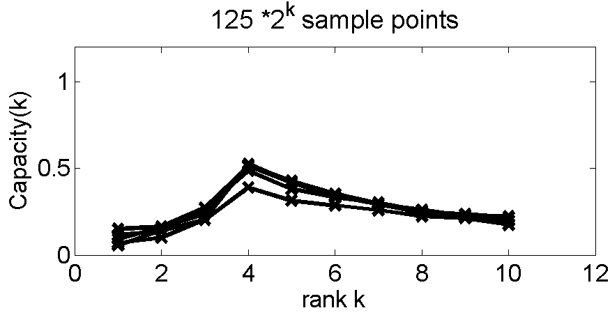
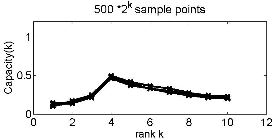
Figure 1: Approximation capacity against rank for various numbers of sample points. The optimal rank is k=4๐‘˜4k=4. Even though the individual trends still vary a lot for very few sample points, the optimal model-order is already found. With increasing number of transformations the calculations are stabilized.

III-B Finite and Bounded Hypothesis space

In the discussion above, we identified two problems: an infinitely large capacity due to i) an infinitely large transformation space โ„Nร—ksuperscriptโ„๐‘๐‘˜\mathbb{R}^{N\times k} (or a negative one if we disregard the infinitely many possible codewords) and ii) due to the existence of infinitely many transformations in an arbitrary small volume of this space. For a practical implementation of the maxAC criterion for SVD we have to i) bound the hypothesis space and ii) constraint the density of transformations to a finite number. This renders the integrals for computing the weight sums to finite sums which must be explicitly computed. In our experiments, we use two ways of summing over the hypothesis space. First, the transformations populate the hypothesis space on an equispaced grid in a hypercube of finite size. Second, we randomly sample transformations from an isotropic Gaussian. In both cases the set of transformations is centered around the cost minimizing solution ๐”(1)superscript๐”1\mathbf{U}^{(1)} (the identity transformation ๐”idsubscript๐”id\mathbf{U}_{\text{id}}). For both ways, one must choose the boundaries (the size of the grid or the variance of the Gaussian) as well as the number of transformations.

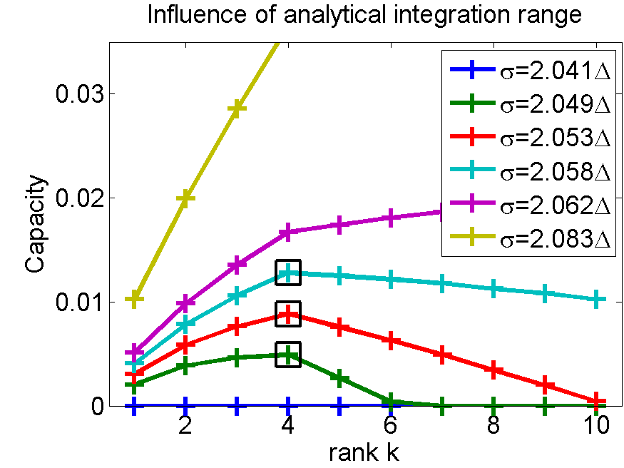
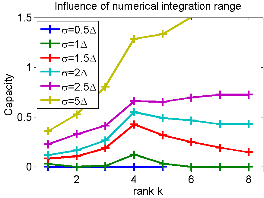
We experimentally investigate the influence of these parameters. First, we study the influence of the integration range on the capacity. We create data ๐—(ฮฝ)superscript๐—๐œˆ\mathbf{X}^{(\nu)} from a mixture of 4 Gaussians with isotropic noise, leading to an optimal rank 4. We compute the approximation capacity by sampling transformations from a Gaussian sphere around the cost-minimizing SVD solution ๐”(ฮฝ)superscript๐”๐œˆ\mathbf{U}^{(\nu)} with standard deviation ฯƒ๐œŽ\sigma. Our experimental findings for various magnitudes of ฯƒ๐œŽ\sigma are illustrated in Fig.ย 2. We write ฯƒ๐œŽ\sigma in units of ฮ”=1/Nโ€‹โˆ‘i=1Nโ€–๐ฎi(1,2)โˆ’๐ฎi(1)โ€–ฮ”1๐‘superscriptsubscript๐‘–1๐‘normsuperscriptsubscript๐ฎ๐‘–12superscriptsubscript๐ฎ๐‘–1\Delta=1/N\sum_{i=1}^{N}\left\|\mathbf{u}_{i}^{(1,2)}-\mathbf{u}_{i}^{(1)}\right\|, whereas ๐”(1,2)superscript๐”12\mathbf{U}^{(1,2)} is the matrix that satisfies ๐—(2)=๐”(1,2)โ€‹๐–(1)superscript๐—2superscript๐”12superscript๐–1\mathbf{X}^{(2)}=\mathbf{U}^{(1,2)}\mathbf{W}^{(1)}. In the regime where 1/Nโ€‹โ€–๐”ฯ„โ€–โ‰ˆฮ”1๐‘normsubscript๐”๐œฮ”1/N\left\|\mathbf{U}_{\tau}\right\|\approx\Delta, a transformed dataset ฯ„jโˆ˜๐—(2)subscript๐œ๐‘—superscript๐—2\tau_{j}\circ\mathbf{X}^{(2)} could possibly be confused with ๐—(1)superscript๐—1\mathbf{X}^{(1)}. When the transformations are smaller than ฮ”ฮ”\Delta, none of the transformations could possibly be used in a codebook as they are all indistinguishable from the identity transformation. As a result, the obtained capacity is too low. On the contrary, for a too high integration range, the capacity converges to the naรฏve analytical solution because infinitely many transformations could serve as distinguishable codewords.
Refer to caption
Figure 2: Numerically computed approximation capacity for various sizes of the subspace containing the transformations.

The second experiment studies the influence of the number of transformations on the mutual information. This time, we use a grid of fixed size and vary the density of grid points. In order to sufficiently cover the hypothesis space, we increase the number of transformations by a factor of 2 when increasing k๐‘˜k. While this increment is still too low to preserve the transformation density, it already imposes a computational challenge. In our experiments with larger datasets, we sample the hypothesis space more sparsely. The influence of the number of transformations is illustrated in Fig.ย 1. The results demonstrate that this number only affects the stability of the computation and not the maximum of the capacity.

III-C Continuous and bounded hypothesis space

The numerical experiment on the influence of the number of transformations suggests that for a defined transformation density, the analytical solution should provide the desired result if only the integration range is properly defined. We calculate the mutual information as in Sectionย III-A but, this time, we weight the integrand with an isotropic Gaussian around the identity uiโ€‹t(1),โˆ€i,tsubscriptsuperscript๐‘ข1๐‘–๐‘กfor-all๐‘–๐‘กu^{(1)}_{it},\forall\>i,t to suppress the contribution of heavy transformations.

๐’ตฮฝsubscript๐’ต๐œˆ\displaystyle\mathcal{Z}_{\nu}\! =โˆซโˆ’โˆžโˆžeโˆ’ฮฒโ€‹Rฮฝโ€‹eโˆ’12โ€‹ฯƒโ€‹โˆ‘i,t(uiโ€‹tโˆ’uiโ€‹tโˆ—)2โ€‹๐‘‘๐”,ฮฝโˆˆ{1,2}formulae-sequenceabsentsuperscriptsubscriptsuperscript๐‘’๐›ฝsubscript๐‘…๐œˆsuperscript๐‘’12๐œŽsubscript๐‘–๐‘กsuperscriptsubscript๐‘ข๐‘–๐‘กsubscriptsuperscript๐‘ข๐‘–๐‘ก2differential-d๐”๐œˆ12\displaystyle=\!\!\int_{-\infty}^{\infty}\!\!\!e^{-\beta R_{\nu}}e^{-\frac{1}{2\sigma}\sum_{i,t}(u_{it}-u^{*}_{it})^{2}}{d\mathbf{U}},\ \nu\in\left\{1,2\right\} (13)
๐’ต12subscript๐’ต12\displaystyle\mathcal{Z}_{12}\! =โˆซโˆ’โˆžโˆžeโˆ’ฮฒโ€‹Rฮ”โ€‹eโˆ’12โ€‹ฯƒโ€‹โˆ‘i,t(uiโ€‹tโˆ’uiโ€‹tโˆ—)2โ€‹๐‘‘๐”absentsuperscriptsubscriptsuperscript๐‘’๐›ฝsubscript๐‘…ฮ”superscript๐‘’12๐œŽsubscript๐‘–๐‘กsuperscriptsubscript๐‘ข๐‘–๐‘กsubscriptsuperscript๐‘ข๐‘–๐‘ก2differential-d๐”\displaystyle=\!\!\int_{-\infty}^{\infty}\!\!\!e^{-\beta R_{\Delta}}e^{-\frac{1}{2\sigma}\sum_{i,t}(u_{it}-u^{*}_{it})^{2}}{d\mathbf{U}} (14)

The derivation of the mutual information is provided in Appendix B. The simulations depicted in Fig.ย 3 illustrate that for an analytically computed mutual information (see Eq.ย (40)), the width ฯƒ๐œŽ\sigma influences the capacity much more than in the numerical computation (compare with Fig.ย 3). However, if a maximum exists (square markers in Fig.ย 3), it is at the correct rank.

Refer to caption
Figure 3: Analytically computed approximation capacity integrated over an isotropic Gaussian sphere with varying standard deviation.

III-D Comparison with other model-selection techniques

We study how well maxAC and other model-order selection methods select the appropriate rank for approximating a noisy dataset via rank-limited SVD. A comparison with the following methods is performed: โ€™Laplaceโ€™ and โ€™BICโ€™ approximate the marginal likelihood (the evidence) for probabilistic PCA [3]. The first method applies Laplace approximation to the involved integral. The well-known BIC score [4] further simplifies that the likelihood exhibits the same sensitivity to all model parameters. A third method, the minimum transfer cost principle (โ€™MTCโ€™) [5], mimics cross-validation. It learns a rank-limited SVD on one random subset of the data and then computes the costs when applying it to another one. Thereby, the model parameters are transfered by a mapping function ฯˆ๐œ“\psi which maps each object in the first dataset to its nearest neighbor in the second dataset.

We create objects from a number of centroids with a defined separation from each other and add Gaussian noise. The difficulty of the problem is controlled by altering the variance relative to the separation of the centroids. When going to a higher number of centroids, the dimensionality must also be increased to preserve their separation. To enable a comparison with the PCA methods, the data mean is shifted to the origin.

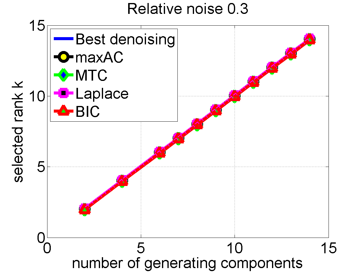
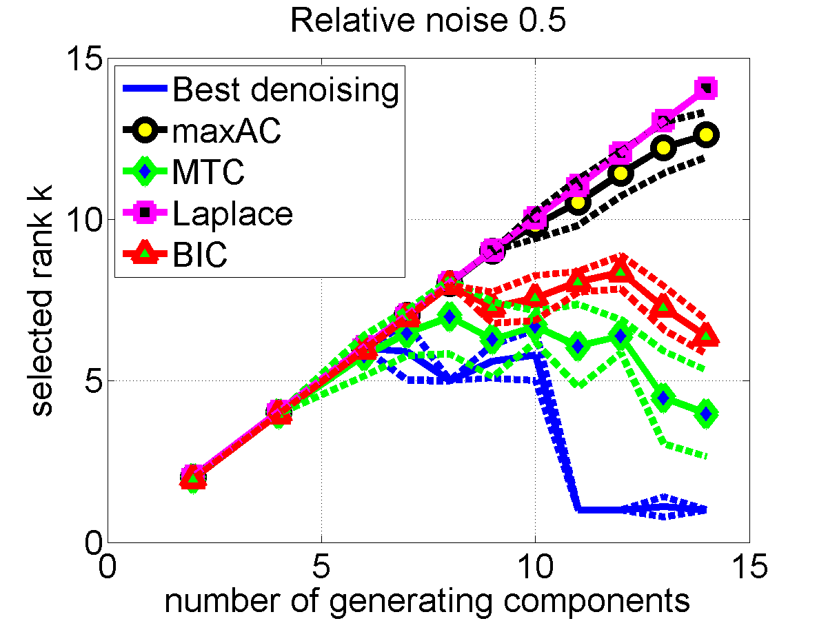
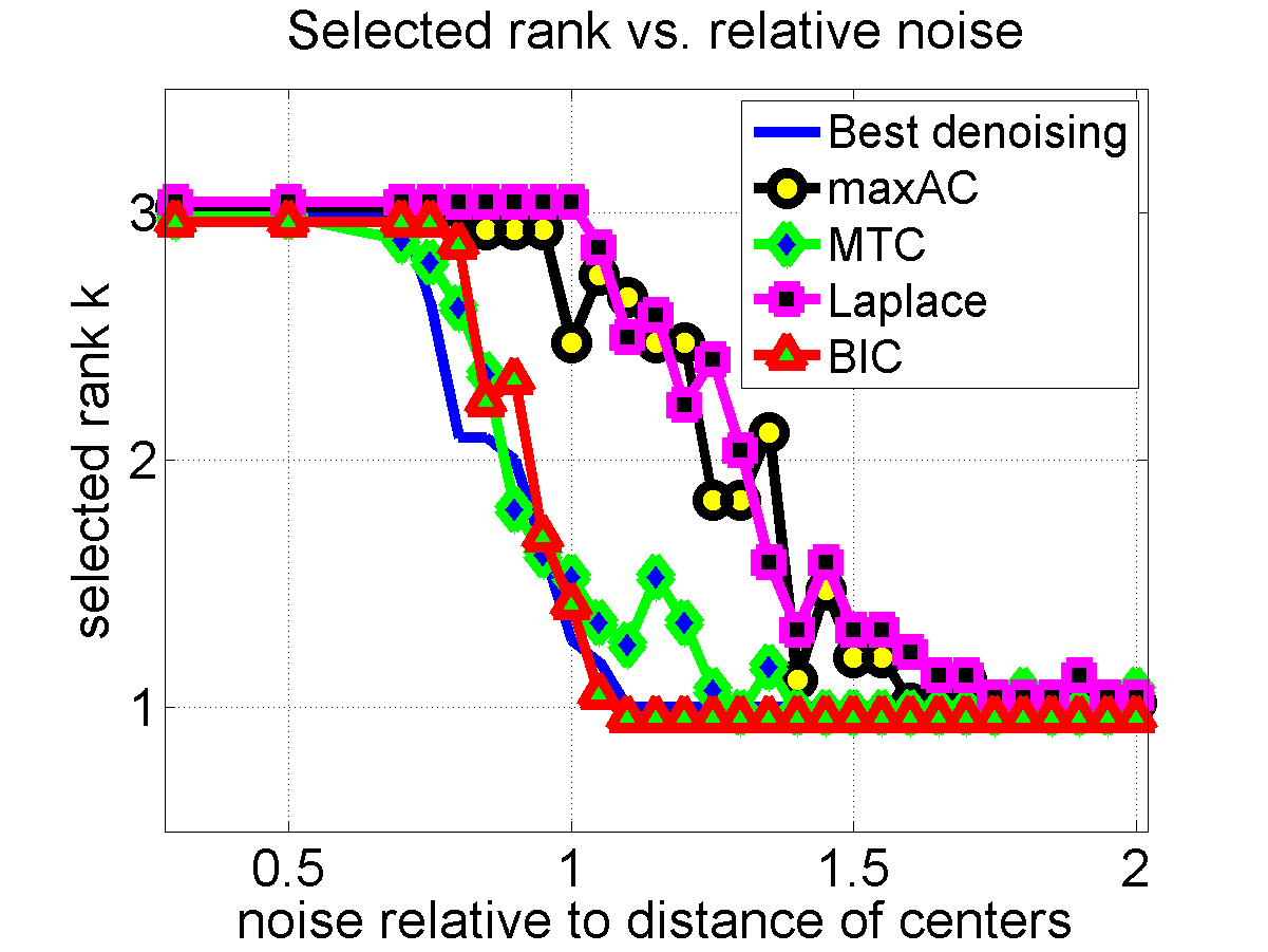
For a given true number of generating components and a given noise level relative to the centroid separation, there exists one SVD rank that yields the reconstruction with the minimal deviation from the noise-free matrix. For very noisy data or a high number of components and dimensions, this optimally denoising rank is smaller than the true number of generating components. Inspecting Fig.ย 4, one can see that all methods select a rank between the best denoising rank and the true rank. For low noise (Fig.ย 4(a)) learning the rank is easy. For a high noise level, the learning problem becomes hard when the number of generating components and the dimensionality increase. There exists a transitional regime where all methods start selecting a lower rank than the true one (Fig.ย 4(b)). For very high noise levels, all methods select k=1๐‘˜1k=1 (Fig.ย 4(c)).

IV Conclusion

We proposed a novel technique for selecting the cut-off rank of truncated SVD. Our criterion selects the rank that maximizes the approximation capacity (maxAC) and, thereby, captures the maximum amount of information in the data that can by reliably inferred from random subsets of the input dataset. We demonstrated, for the first time, how to apply maxAC to an optimization problem with a continuous solution space like SVD. The Euclidean geometry of the parameter space renders the computation of the approximation capacity more difficult than in the clustering case with random permutations [2]. We discussed the challenges with such problem domains and proposed solutions. Finally, we demonstrated in comparative experiments that the model-order selection of our technique conforms with established methods. Future work will address the application of the maxAC criterion to other continuous optimization problems such as, for instance, sparse linear regression.

Acknowledgments

This work was partially supported by the Zurich Information Security Center and by the FP7 EU project SIMBAD.

References

  • [1] J.ย M. Buhmann, โ€œInformation theoretic model validation for clustering,โ€ in ISIT, 2010.
  • [2] J.ย M. Buhmann, M.ย H. Chehreghani, M.ย Frank, and A.ย P. Streich, โ€œInformation theoretic model selection for pattern analysis,โ€ in JMLR: Workshop and Conference Proceedings 7, 1-8, 2011.
  • [3] T.ย P. Minka, โ€œAutomatic choice of dimensionality for PCA,โ€ in NIPS, 2000, p. 514.
  • [4] G.ย Schwarz, โ€œEstimating the dimension of a model,โ€ The Annals of Statistics, vol.ย 6, no.ย 2, pp. 461โ€“464, 1978.
  • [5] M.ย Frank, M.ย H. Chehreghani, and J.ย M. Buhmann, โ€œThe minimum transfer cost principle for model-order selection,โ€ in ECML, 2011.
Refer to caption
(a) Low relative noise
Refer to caption
(b) High relative noise
Refer to caption
(c) Various noise levels
Figure 4: Rank-k approximation for a mixture of Gaussians. In (a) and (b) the number of generating components varies, in (c) the noise level varies for 3 components. For readability, we omitted the variances in (c). They are comparable with (b). All methods select a rank between the true number of components and the rank that minimizes the distance to the noise-free matrix (โ€˜Best denoisingโ€™).

Appendix A: attaining capacity

There are several ways of numerically maximizing the mutual information in Eq.ย 4 with respect to the temperature. The simplest way is to compute Iฮฒsubscript๐ผ๐›ฝI_{\beta} for several values of ฮฒ๐›ฝ\beta and pick the maximum. This creates a quantization error of the optimum that depends on the step-size of the temperature scale. Moderate step-sizes already lead to good results as Iฮฒsubscript๐ผ๐›ฝI_{\beta} is usually flat around its maximum.

Using a gradient-descent method like Newton iterations provide more precise results . In the following, we report the first and the second derivation of Iฮฒsubscript๐ผ๐›ฝI_{\beta} which are needed for the Newton updates. The derivation of the mutual information Iฮฒsubscript๐ผ๐›ฝI_{\beta} (Eq.ย 4) with respect to the inverse temperature ฮฒ๐›ฝ\beta is

โˆ‚Iโ€‹(ฮฒ)โˆ‚ฮฒ=1/Nโ€‹โˆ‚โˆ‚ฮฒโ€‹(logโก(|ฮ”โ€‹Cฮณ|)โˆ’โˆ‘ฮฝ=12logโก(|Cฮณ(ฮฝ)|))๐ผ๐›ฝ๐›ฝ1๐‘๐›ฝฮ”subscript๐ถ๐›พsuperscriptsubscript๐œˆ12subscriptsuperscript๐ถ๐œˆ๐›พ\displaystyle\frac{\partial I(\beta)}{\partial\beta}=1/N\frac{\partial}{\partial\beta}\left(\log\left(\left|\Delta C_{\gamma}\right|\right)-\sum_{\nu=1}^{2}\log\left(\left|C^{(\nu)}_{\gamma}\right|\right)\right) (15)
=1/Nโ€‹(1|ฮ”โ€‹Cฮณ|โ€‹โˆ‚โˆ‚ฮฒโ€‹|ฮ”โ€‹Cฮณ|โˆ’โˆ‘ฮฝ=121|Cฮณ(ฮฝ)|โ€‹โˆ‚โˆ‚ฮฒโ€‹|Cฮณ(ฮฝ)|)absent1๐‘1ฮ”subscript๐ถ๐›พ๐›ฝฮ”subscript๐ถ๐›พsuperscriptsubscript๐œˆ121subscriptsuperscript๐ถ๐œˆ๐›พ๐›ฝsubscriptsuperscript๐ถ๐œˆ๐›พ\displaystyle=\!\!1/N\left(\frac{1}{\left|\Delta C_{\gamma}\right|}\frac{\partial}{\partial\beta}\left|\Delta C_{\gamma}\right|-\sum_{\nu=1}^{2}\frac{1}{\left|C^{(\nu)}_{\gamma}\right|}\frac{\partial}{\partial\beta}\left|C^{(\nu)}_{\gamma}\right|\right) (16)
=1/Nโ€‹(โˆ‘ฮฝ=12(โˆซโˆ’โˆžโˆžRฮฝโ€‹expโก[โˆ’ฮฒโ€‹Rฮฝ]โ€‹๐‘‘๐”โˆซโˆ’โˆžโˆžexpโก[โˆ’ฮฒโ€‹Rฮฝ]โ€‹๐‘‘๐”)โˆ’โˆซโˆ’โˆžโˆžRฮ”โ€‹expโก[โˆ’ฮฒโ€‹Rฮ”]โ€‹๐‘‘๐”โˆซโˆ’โˆžโˆžexpโก[โˆ’ฮฒโ€‹Rฮ”]โ€‹๐‘‘๐”)absent1๐‘superscriptsubscript๐œˆ12superscriptsubscriptsubscript๐‘…๐œˆ๐›ฝsubscript๐‘…๐œˆdifferential-d๐”superscriptsubscript๐›ฝsubscript๐‘…๐œˆdifferential-d๐”superscriptsubscriptsubscript๐‘…ฮ”๐›ฝsubscript๐‘…ฮ”differential-d๐”superscriptsubscript๐›ฝsubscript๐‘…ฮ”differential-d๐”\displaystyle=\!\!1/N\!\!\left(\sum_{\nu=1}^{2}\!\!\left(\frac{\!\!\int_{-\infty}^{\infty}\!\!\!R_{\nu}\exp\left[-\beta R_{\nu}\right]{d\mathbf{U}}}{\!\!\int_{-\infty}^{\infty}\!\!\!\exp\left[-\beta R_{\nu}\right]{d\mathbf{U}}}\right)\!\!-\frac{\!\!\int_{-\infty}^{\infty}\!\!\!R_{\Delta}\exp\left[-\beta R_{\Delta}\right]{d\mathbf{U}}}{\!\!\int_{-\infty}^{\infty}\!\!\!\exp\left[-\beta R_{\Delta}\right]{d\mathbf{U}}}\right)
=1/Nโ€‹(โˆ‘ฮฝ=12๐”ผโ€‹[Rฮฝ]pGโ€‹(Rฮฝ)โˆ’๐”ผโ€‹[Rฮ”]pGโ€‹(Rฮ”))absent1๐‘superscriptsubscript๐œˆ12๐”ผsubscriptdelimited-[]subscript๐‘…๐œˆsubscript๐‘๐บsubscript๐‘…๐œˆ๐”ผsubscriptdelimited-[]subscript๐‘…ฮ”subscript๐‘๐บsubscript๐‘…ฮ”\displaystyle=\!\!1/N\left(\sum_{\nu=1}^{2}\mathbb{E}[R_{\nu}]_{p_{G}(R_{\nu})}-\mathbb{E}[R_{\Delta}]_{p_{G}(R_{\Delta})}\right) (17)

Where pGโ€‹(Rฮ”)=Zโˆ’1โ€‹expโก(โˆ’ฮฒโ€‹Rฮ”)subscript๐‘๐บsubscript๐‘…ฮ”superscript๐‘1๐›ฝsubscript๐‘…ฮ”p_{G}(R_{\Delta})=Z^{-1}\exp(-\beta R_{\Delta}) is the Gibbs distribution with normalization constant Z=โˆซโˆ’โˆžโˆžexpโก[โˆ’ฮฒโ€‹Rฮ”]โ€‹๐‘‘๐”๐‘superscriptsubscript๐›ฝsubscript๐‘…ฮ”differential-d๐”Z=\int_{-\infty}^{\infty}\!\!\!\exp\left[-\beta R_{\Delta}\right]{d\mathbf{U}}. These expectations can easily be computed either for a finite set of transformations or with a continuous integral.

Accordingly, the second derivative is:

โˆ‚2Iโ€‹(ฮฒ)โˆ‚ฮฒ2=1/N(โˆ‘ฮฝ=12(โˆ‚โˆ‚ฮฒโˆซโˆ’โˆžโˆžRฮฝโ€‹expโก[โˆ’ฮฒโ€‹Rฮฝ]โ€‹๐‘‘๐”โˆซโˆ’โˆžโˆžexpโก[โˆ’ฮฒโ€‹Rฮฝ]โ€‹๐‘‘๐”)\displaystyle\frac{\partial^{2}I(\beta)}{\partial\beta^{2}}=1/N\left(\sum_{\nu=1}^{2}\left(\frac{\partial}{\partial\beta}\frac{\!\!\int_{-\infty}^{\infty}\!\!\!R_{\nu}\exp\left[-\beta R_{\nu}\right]{d\mathbf{U}}}{\!\!\int_{-\infty}^{\infty}\!\!\!\exp\left[-\beta R_{\nu}\right]{d\mathbf{U}}}\right)\right.
โˆ’โˆ‚โˆ‚ฮฒโˆซโˆ’โˆžโˆžRฮ”โ€‹expโก[โˆ’ฮฒโ€‹Rฮ”]โ€‹๐‘‘๐”โˆซโˆ’โˆžโˆžexpโก[โˆ’ฮฒโ€‹Rฮ”]โ€‹๐‘‘๐”)\displaystyle\quad\quad\quad\left.-\frac{\partial}{\partial\beta}\frac{\!\!\int_{-\infty}^{\infty}\!\!\!R_{\Delta}\exp\left[-\beta R_{\Delta}\right]{d\mathbf{U}}}{\!\!\int_{-\infty}^{\infty}\!\!\!\exp\left[-\beta R_{\Delta}\right]{d\mathbf{U}}}\right) (18)
=1/Nโ€‹(โˆ‘ฮฝ=12(๐”ผโ€‹[Rฮฝ]pGโ€‹(Rฮฝ)2โˆ’๐”ผโ€‹[Rฮฝ2]pGโ€‹(Rฮฝ)))absent1๐‘superscriptsubscript๐œˆ12๐”ผsuperscriptsubscriptdelimited-[]subscript๐‘…๐œˆsubscript๐‘๐บsubscript๐‘…๐œˆ2๐”ผsubscriptdelimited-[]subscriptsuperscript๐‘…2๐œˆsubscript๐‘๐บsubscript๐‘…๐œˆ\displaystyle=\!\!1/N\left(\sum_{\nu=1}^{2}\left(\mathbb{E}[R_{\nu}]_{p_{G}(R_{\nu})}^{2}-\mathbb{E}[R^{2}_{\nu}]_{p_{G}(R_{\nu})}\right)\right)
โˆ’1/Nโ€‹(๐”ผโ€‹[Rฮ”2]pGโ€‹(Rฮ”)โˆ’๐”ผโ€‹[Rฮ”]pGโ€‹(Rฮ”)2)1๐‘๐”ผsubscriptdelimited-[]subscriptsuperscript๐‘…2ฮ”subscript๐‘๐บsubscript๐‘…ฮ”๐”ผsuperscriptsubscriptdelimited-[]subscript๐‘…ฮ”subscript๐‘๐บsubscript๐‘…ฮ”2\displaystyle\quad\quad\quad-1/N\left(\mathbb{E}[R^{2}_{\Delta}]_{p_{G}(R_{\Delta})}-\mathbb{E}[R_{\Delta}]_{p_{G}(R_{\Delta})}^{2}\right) (19)

Appendix B: Analytical Calculation with bounded integration range

We derive the mutual information Eq.ย (40) when the transformations are weighted with a Gaussian centered around the identity transformation uiโ€‹t(1)subscriptsuperscript๐‘ข1๐‘–๐‘กu^{(1)}_{it}. Except for this modification the derivation is analog to the derivation of the unconstraint mutual information in Eq.ย (11). The approximation sets and the joint approximation set are

|Cฮณ(ฮฝ)|subscriptsuperscript๐ถ๐œˆ๐›พ\displaystyle\left|C^{(\nu)}_{\gamma}\right| =\displaystyle= โˆซโˆ’โˆžโˆžexpโก(โˆ’ฮฒโ€‹Rโ€‹(๐—(ฮฝ),๐”,๐’(ฮฝ),๐•(ฮฝ)))โ€‹expโก(โˆ’12โ€‹ฯƒโ€‹โˆ‘i,t(uiโ€‹tโˆ’uiโ€‹t(1))2)โ€‹๐‘‘๐”,ฮฝโˆˆ{1,2}superscriptsubscript๐›ฝ๐‘…superscript๐—๐œˆ๐”superscript๐’๐œˆsuperscript๐•๐œˆ12๐œŽsubscript๐‘–๐‘กsuperscriptsubscript๐‘ข๐‘–๐‘กsubscriptsuperscript๐‘ข1๐‘–๐‘ก2differential-d๐”๐œˆ12\displaystyle\int_{-\infty}^{\infty}\exp\left(-\beta R(\mathbf{X}^{(\nu)},\mathbf{U},\mathbf{S}^{(\nu)},\mathbf{V}^{(\nu)})\right)\exp\left(-\frac{1}{2\sigma}\sum_{i,t}(u_{it}-u^{(1)}_{it})^{2}\right){d\mathbf{U}}\ ,\nu\in\left\{1,2\right\} (20)
=\displaystyle= โˆiโ€‹jexpโก(โˆ’ฮฒโ€‹xiโ€‹j(ฮฝ)2)โ€‹expโก(โˆ’12โ€‹ฯƒโ€‹Dโ€‹โˆ‘tuiโ€‹tโˆ—2)subscriptproduct๐‘–๐‘—๐›ฝsuperscriptsuperscriptsubscript๐‘ฅ๐‘–๐‘—๐œˆ212๐œŽ๐ทsubscript๐‘กsuperscriptsubscript๐‘ข๐‘–๐‘กabsent2\displaystyle\prod_{ij}\exp\left(-\beta{x_{ij}^{(\nu)}}^{2}\right)\exp\left(-\frac{1}{2\sigma D}\sum_{t}u_{it}^{*2}\right)
โ‹…โˆซโˆ’โˆžโˆžexp(โˆ’ฮฒโˆ‘tkuiโ€‹t(1ฯƒโ€‹ฮฒโ€‹Duiโ€‹t(1)โˆ’2xiโ€‹j(ฮฝ)wtโ€‹j(ฮฝ)))\displaystyle\quad\cdot\int_{-\infty}^{\infty}\exp\left(-\beta\sum_{t}^{k}u_{it}\left(\frac{1}{\sigma\beta D}u^{(1)}_{it}-2x_{ij}^{(\nu)}w_{tj}^{(\nu)}\right)\right)
โ‹…expโก(โˆ’2โ€‹ฮฒโ€‹โˆ‘tkuiโ€‹tโ€‹(wtโ€‹j(ฮฝ)โ€‹2โ€‹uiโ€‹t+2โ€‹wtโ€‹j(ฮฝ)โ€‹โˆ‘tโ€ฒโ‰ tkuiโ€‹tโ€ฒโ€‹wtโ€ฒโ€‹j(ฮฝ)+12โ€‹ฯƒโ€‹ฮฒโ€‹Dโ€‹uiโ€‹t))โ€‹dkโ€‹๐ฎ๐ข,.\displaystyle\quad\quad\quad\>\cdot\exp\left(-2\beta\sum_{t}^{k}u_{it}\left(w_{tj}^{(\nu)2}u_{it}+2w_{tj}^{(\nu)}\sum_{t^{\prime}\neq t}^{k}u_{it^{\prime}}w_{t^{\prime}j}^{(\nu)}+\frac{1}{2\sigma\beta D}u_{it}\right)\right){d^{k}\mathbf{u_{i,.}}}

and

|ฮ”โ€‹Cฮณ|ฮ”subscript๐ถ๐›พ\displaystyle\left|\Delta C_{\gamma}\right| =\displaystyle= โˆซโˆ’โˆžโˆžexpโก(โˆ’ฮฒ/2โ€‹(Rโ€‹(๐—(1),๐”,๐’(1),๐•(1))+Rโ€‹(๐—(2),๐”,๐’(1),๐•(1))))โ€‹expโก(โˆ’12โ€‹ฯƒโ€‹โˆ‘i,t(uiโ€‹tโˆ’uiโ€‹t(1))2)โ€‹๐‘‘๐”superscriptsubscript๐›ฝ2๐‘…superscript๐—1๐”superscript๐’1superscript๐•1๐‘…superscript๐—2๐”superscript๐’1superscript๐•112๐œŽsubscript๐‘–๐‘กsuperscriptsubscript๐‘ข๐‘–๐‘กsubscriptsuperscript๐‘ข1๐‘–๐‘ก2differential-d๐”\displaystyle\int_{-\infty}^{\infty}\exp\left(-\beta/2\left(R(\mathbf{X}^{(1)},\mathbf{U},\mathbf{S}^{(1)},\mathbf{V}^{(1)})+R(\mathbf{X}^{(2)},\mathbf{U},\mathbf{S}^{(1)},\mathbf{V}^{(1)})\right)\right)\exp\left(-\frac{1}{2\sigma}\sum_{i,t}(u_{it}-u^{(1)}_{it})^{2}\right){d\mathbf{U}} (22)
=\displaystyle= โˆiโ€‹jexpโก(โˆ’ฮฒ/2โ€‹(xiโ€‹j(1)2+xiโ€‹j(2)2))โ€‹expโก(โˆ’12โ€‹ฯƒโ€‹Dโ€‹โˆ‘tuiโ€‹tโˆ—2)subscriptproduct๐‘–๐‘—๐›ฝ2superscriptsuperscriptsubscript๐‘ฅ๐‘–๐‘—12superscriptsuperscriptsubscript๐‘ฅ๐‘–๐‘—2212๐œŽ๐ทsubscript๐‘กsuperscriptsubscript๐‘ข๐‘–๐‘กabsent2\displaystyle\prod_{ij}\exp\left(-\beta/2\left({x_{ij}^{(1)}}^{2}+{x_{ij}^{(2)}}^{2}\right)\right)\exp\left(-\frac{1}{2\sigma D}\sum_{t}u_{it}^{*2}\right)
โ‹…โˆซโˆ’โˆžโˆžexp(โˆ’ฮฒโˆ‘tkuiโ€‹t(wtโ€‹j(1)โ€‹2uiโ€‹t+2wtโ€‹j(1)โˆ‘tโ€ฒโ‰ tkuiโ€‹tโ€ฒwtโ€ฒโ€‹j(1)+12โ€‹ฯƒโ€‹ฮฒโ€‹Duiโ€‹t))\displaystyle\quad\cdot\int_{-\infty}^{\infty}\exp\left(-\beta\sum_{t}^{k}u_{it}\left(w_{tj}^{(1)2}u_{it}+2w_{tj}^{(1)}\sum_{t^{\prime}\neq t}^{k}u_{it^{\prime}}w_{t^{\prime}j}^{(1)}+\frac{1}{2\sigma\beta D}u_{it}\right)\right)
โ‹…expโก(โˆ’ฮฒโ€‹โˆ‘tkuiโ€‹tโ€‹((xiโ€‹j(1)+xiโ€‹j(2))โ€‹wtโ€‹j(1)โˆ’1ฯƒโ€‹ฮฒโ€‹Dโ€‹uiโ€‹t(1)))โ€‹dkโ€‹๐ฎ๐ข,..\displaystyle\quad\quad\quad\>\cdot\exp\left(-\beta\sum_{t}^{k}u_{it}\left((x_{ij}^{(1)}+x_{ij}^{(2)})w_{tj}^{(1)}-\frac{1}{\sigma\beta D}u^{(1)}_{it}\right)\right){d^{k}\mathbf{u_{i,.}}}\ .

The characteristic terms of the integrals are

๐€(๐ฃ)(ฮฝ)=2โ€‹ฮฒโ€‹๐š(๐ฃ)(ฮฝ),subscriptsuperscript๐€๐œˆ๐ฃ2๐›ฝsubscriptsuperscript๐š๐œˆ๐ฃ\displaystyle\mathbf{A^{(\nu)}_{(j)}}=2\beta\mathbf{a^{(\nu)}_{(j)}}, (24)
๐›(๐ข,๐ฃ)(ฮฝ)=2โ€‹ฮฒโ€‹xiโ€‹j(ฮฝ)โ€‹๐ฐ.,๐ฃ(ฮฝ)Tโˆ’1ฯƒโ€‹Dโ€‹๐ฎ๐ข,.(๐Ÿ),\displaystyle\mathbf{b^{(\nu)}_{(i,j)}}=2\beta\;x_{ij}^{(\nu)}\mathbf{w_{.,j}^{(\nu)}}^{T}-\frac{1}{\sigma D}\mathbf{u^{(1)}_{i,.}}\ , (25)
๐€(๐ฃ)(๐šซ)=๐€(๐ฃ)(๐Ÿ),subscriptsuperscript๐€๐šซ๐ฃsubscriptsuperscript๐€1๐ฃ\displaystyle\mathbf{A^{(\Delta)}_{(j)}}=\mathbf{A^{(1)}_{(j)}}\ , (26)
๐›(๐ข,๐ฃ)(๐šซ)=ฮฒโ€‹(xiโ€‹j(1)+xiโ€‹j(2))โ€‹๐ฐ.,๐ฃ(๐Ÿ)Tโˆ’1ฯƒโ€‹Dโ€‹๐ฎ๐ข,.(๐Ÿ),\displaystyle\mathbf{b^{(\Delta)}_{(i,j)}}=\beta\;\left(x_{ij}^{(1)}+x_{ij}^{(2)}\right)\mathbf{w_{.,j}^{(1)}}^{T}-\frac{1}{\sigma D}\mathbf{u^{(1)}_{i,.}}\ , (27)

with

๐š(๐ฃ)(ฮฝ):=๐ฐ.,๐ฃ(ฮฝ)Tโ€‹๐ฐ.,๐ฃ(ฮฝ)+12โ€‹ฯƒโ€‹ฮฒโ€‹Dโ€‹๐•€.\displaystyle\mathbf{a^{(\nu)}_{(j)}}:=\mathbf{w_{.,j}^{(\nu)}}^{T}\mathbf{w_{.,j}^{(\nu)}}+\frac{1}{2\sigma\beta D}\mathbb{I}\ . (28)

These terms determine the cardinalities of the approximation sets:

|Cฮณ(ฮฝ)|subscriptsuperscript๐ถ๐œˆ๐›พ\displaystyle\left|C^{(\nu)}_{\gamma}\right| =\displaystyle= โˆi,jexpโก(โˆ’ฮฒโ€‹xiโ€‹j(ฮฝ)โ€‹2)โ€‹expโก(โˆ’12โ€‹ฯƒโ€‹Dโ€‹๐ฎ๐ข,.(๐Ÿ)โ€‹๐ฎ๐ข,.(๐Ÿ)T)โ€‹(2โ€‹ฯ€)kdet(2โ€‹ฮฒโ€‹๐š(๐ฃ)(ฮฝ))โ€‹expโก(12โ€‹๐›(๐ข,๐ฃ)(ฮฝ)Tโ€‹๐€(๐ฃ)(ฮฝ)โˆ’1โ€‹๐›(๐ข,๐ฃ)(ฮฝ))\displaystyle\prod_{i,j}\exp\left(-\beta x_{ij}^{(\nu)2}\right)\exp\left(-\frac{1}{2\sigma D}\mathbf{u^{(1)}_{i,.}}\mathbf{u^{(1)}_{i,.}}^{T}\right)\sqrt{\frac{(2\pi)^{k}}{\det\left(2\beta\mathbf{a^{(\nu)}_{(j)}}\right)}}\exp\left(\frac{1}{2}\mathbf{b^{(\nu)}_{(i,j)}}^{T}\mathbf{A^{(\nu)}_{(j)}}^{-1}\mathbf{b^{(\nu)}_{(i,j)}}\right) (29)
=\displaystyle= (ฯ€ฮฒ)Nโ€‹Dโ€‹k2โ€‹โˆi,jdet(๐š(๐ฃ)(ฮฝ))โˆ’1/2superscript๐œ‹๐›ฝ๐‘๐ท๐‘˜2subscriptproduct๐‘–๐‘—superscriptsubscriptsuperscript๐š๐œˆ๐ฃ12\displaystyle\left(\frac{\pi}{\beta}\right)^{\frac{NDk}{2}}\!\!\prod_{i,j}\det\left(\mathbf{a^{(\nu)}_{(j)}}\right)^{-1/2}
expโก(โˆ’ฮฒโ€‹xiโ€‹j(ฮฝ)โ€‹2โˆ’12โ€‹ฯƒโ€‹Dโ€‹๐ฎ๐ข,.(๐Ÿ)โ€‹๐ฎ๐ข,.(๐Ÿ)T+14โ€‹ฮฒโ€‹(2โ€‹ฮฒโ€‹xiโ€‹j(ฮฝ)โ€‹๐ฐ.,๐ฃ(ฮฝ)Tโˆ’1ฯƒโ€‹Dโ€‹๐ฎ๐ข,.(๐Ÿ))Tโ€‹๐š(๐ฃ)(ฮฝ)โˆ’1โ€‹(2โ€‹ฮฒโ€‹xiโ€‹j(ฮฝ)โ€‹๐ฐ.,๐ฃ(ฮฝ)Tโˆ’1ฯƒโ€‹Dโ€‹๐ฎ๐ข,.(๐Ÿ)))\displaystyle\!\!\exp\left(-\beta x_{ij}^{(\nu)2}-\frac{1}{2\sigma D}\mathbf{u^{(1)}_{i,.}}\mathbf{u^{(1)}_{i,.}}^{T}+\frac{1}{4\beta}(2\beta\;x_{ij}^{(\nu)}\mathbf{w_{.,j}^{(\nu)}}^{T}-\frac{1}{\sigma D}\mathbf{u^{(1)}_{i,.}})^{T}\mathbf{a^{(\nu)}_{(j)}}^{-1}(2\beta\;x_{ij}^{(\nu)}\mathbf{w_{.,j}^{(\nu)}}^{T}-\frac{1}{\sigma D}\mathbf{u^{(1)}_{i,.}})\right)
=\displaystyle= (ฯ€ฮฒ)Nโ€‹Dโ€‹k2โ€‹(โˆjdet(๐š(๐ฃ)(ฮฝ)))โˆ’N/2superscript๐œ‹๐›ฝ๐‘๐ท๐‘˜2superscriptsubscriptproduct๐‘—subscriptsuperscript๐š๐œˆ๐ฃ๐‘2\displaystyle\left(\frac{\pi}{\beta}\right)^{\frac{NDk}{2}}\left(\prod_{j}\det\left(\mathbf{a^{(\nu)}_{(j)}}\right)\right)^{-N/2}
โ‹…โˆi,jexp(โˆ’ฮฒxiโ€‹j(ฮฝ)โ€‹2(1โˆ’๐ฐ.,๐ฃ(ฮฝ)๐š(๐ฃ)(ฮฝ)โˆ’1๐ฐ.,๐ฃ(ฮฝ)T)โˆ’12โ€‹ฯƒโ€‹D๐ฎ๐ข,.(๐Ÿ)๐ฎ๐ข,.(๐Ÿ)Tโˆ’14โ€‹ฮฒโ€‹ฯƒ2โ€‹D2๐ฎ๐ข,.(๐Ÿ)๐š(๐ฃ)(ฮฝ)โˆ’1๐ฎ๐ข,.(๐Ÿ)T)\displaystyle\cdot\prod_{i,j}\exp\left(-\beta x_{ij}^{(\nu)2}\left(1-\mathbf{w_{.,j}^{(\nu)}}\mathbf{a^{(\nu)}_{(j)}}^{-1}\mathbf{w_{.,j}^{(\nu)}}^{T}\right)-\frac{1}{2\sigma D}\mathbf{u^{(1)}_{i,.}}\mathbf{u^{(1)}_{i,.}}^{T}-\frac{1}{4\beta\sigma^{2}D^{2}}\mathbf{u^{(1)}_{i,.}}\mathbf{a^{(\nu)}_{(j)}}^{-1}\mathbf{u^{(1)}_{i,.}}^{T}\right)

and

|ฮ”โ€‹Cฮณ|ฮ”subscript๐ถ๐›พ\displaystyle\left|\Delta C_{\gamma}\right| =โˆi,jexpโก(โˆ’ฮฒ2โ€‹(xiโ€‹j(1)โ€‹2+xiโ€‹j(2)โ€‹2))โ€‹expโก(โˆ’12โ€‹ฯƒโ€‹Dโ€‹๐ฎ๐ข,.(๐Ÿ)โ€‹๐ฎ๐ข,.(๐Ÿ)T)โ€‹(2โ€‹ฯ€)kdet(2โ€‹ฮฒโ€‹๐š(๐ฃ)(๐Ÿ))โ€‹expโก(12โ€‹๐›(๐ข,๐ฃ)(๐šซ)Tโ€‹๐€(๐ฃ)(๐Ÿ)โˆ’1โ€‹๐›(๐ข,๐ฃ)(๐šซ))\displaystyle\!\!=\!\!\prod_{i,j}\exp\left(-\frac{\beta}{2}\left(x_{ij}^{(1)2}+x_{ij}^{(2)2}\right)\right)\exp\left(-\frac{1}{2\sigma D}\mathbf{u^{(1)}_{i,.}}\mathbf{u^{(1)}_{i,.}}^{T}\right)\sqrt{\frac{(2\pi)^{k}}{\det\left(2\beta\mathbf{a^{(1)}_{(j)}}\right)}}\exp\left(\frac{1}{2}\mathbf{b^{(\Delta)}_{(i,j)}}^{T}\mathbf{A^{(1)}_{(j)}}^{-1}\mathbf{b^{(\Delta)}_{(i,j)}}\right) (32)
=(ฯ€ฮฒ)Nโ€‹Dโ€‹k2โ€‹โˆjdet(๐š(๐ฃ)(๐Ÿ))โˆ’N/2absentsuperscript๐œ‹๐›ฝ๐‘๐ท๐‘˜2subscriptproduct๐‘—superscriptsubscriptsuperscript๐š1๐ฃ๐‘2\displaystyle\!\!=\!\!\left(\frac{\pi}{\beta}\right)^{\frac{NDk}{2}}\!\!\!\prod_{j}\det\left(\mathbf{a^{(1)}_{(j)}}\right)^{-N/2} (33)
โˆi,jexpโก(โˆ’ฮฒ2โ€‹(xiโ€‹j(1)โ€‹2+xiโ€‹j(2)โ€‹2โˆ’12โ€‹(xiโ€‹j(1)+xiโ€‹j(2))2โ€‹๐ฐ.,๐ฃ(๐Ÿ)โ€‹๐š(๐ฃ)(๐Ÿ)โˆ’1โ€‹๐ฐ.,๐ฃ(๐Ÿ)T)โˆ’12โ€‹ฯƒโ€‹Dโ€‹๐ฎ๐ข,.(๐Ÿ)โ€‹๐ฎ๐ข,.(๐Ÿ)Tโˆ’14โ€‹ฮฒโ€‹ฯƒ2โ€‹D2โ€‹๐ฎ๐ข,.(๐Ÿ)โ€‹๐š(๐ฃ)(๐Ÿ)โˆ’1โ€‹๐ฎ๐ข,.(๐Ÿ)T)\displaystyle\prod_{i,j}\exp\left(-\frac{\beta}{2}\left(x_{ij}^{(1)2}+x_{ij}^{(2)2}-\frac{1}{2}\left(x_{ij}^{(1)}+x_{ij}^{(2)}\right)^{2}\mathbf{w_{.,j}^{(1)}}\mathbf{a^{(1)}_{(j)}}^{-1}\mathbf{w_{.,j}^{(1)}}^{T}\right)-\frac{1}{2\sigma D}\mathbf{u^{(1)}_{i,.}}\mathbf{u^{(1)}_{i,.}}^{T}\!-\frac{1}{4\beta\sigma^{2}D^{2}}\mathbf{u^{(1)}_{i,.}}\mathbf{a^{(1)}_{(j)}}^{-1}\mathbf{u^{(1)}_{i,.}}^{T}\right)

The number of random transformations depends on the size of the Gaussian sphere b๐‘b :

b๐‘\displaystyle b =\displaystyle= โˆซโˆ’โˆžโˆžexpโก(โˆ’12โ€‹ฯƒโ€‹โˆ‘i,t(uiโ€‹tโˆ’uiโ€‹t(1))2)โ€‹๐‘‘๐”superscriptsubscript12๐œŽsubscript๐‘–๐‘กsuperscriptsubscript๐‘ข๐‘–๐‘กsubscriptsuperscript๐‘ข1๐‘–๐‘ก2differential-d๐”\displaystyle\int_{-\infty}^{\infty}\exp\left(-\frac{1}{2\sigma}\sum_{i,t}(u_{it}-u^{(1)}_{it})^{2}\right){d\mathbf{U}} (34)
=\displaystyle= โˆi(2โ€‹ฯ€)kdet(ฯƒโˆ’1โ€‹๐•€)subscriptproduct๐‘–superscript2๐œ‹๐‘˜superscript๐œŽ1๐•€\displaystyle\prod_{i}\sqrt{\frac{(2\pi)^{k}}{\det\left(\sigma^{-1}\mathbb{I}\right)}} (35)
=\displaystyle= (2โ€‹ฯ€โ€‹ฯƒ)Nโ€‹k2.superscript2๐œ‹๐œŽ๐‘๐‘˜2\displaystyle\left(2\pi\sigma\right)^{\frac{Nk}{2}}\ . (36)

Define the auxiliary variables ๐…(๐ฃ)(ฮฝ):=๐ฐ.,๐ฃ(ฮฝ)โ€‹๐š(๐ฌ)(ฮฝ)โˆ’1โ€‹๐ฐ.,๐ฃ(ฮฝ)T\mathbf{F^{(\nu)}_{(j)}}:=\mathbf{w_{.,j}^{(\nu)}}\mathbf{a^{(\nu)}_{(s)}}^{-1}\mathbf{w_{.,j}^{(\nu)}}^{T}. Then, the mutual information is

Iโ€‹(ฮฒ)๐ผ๐›ฝ\displaystyle I(\beta) =\displaystyle= 1/Nโ€‹(|{ฯ„j}|+logโก(|ฮ”โ€‹Cฮณ|)โˆ’โˆ‘ฮฝ=12logโก(|Cฮณ(ฮฝ)|))1๐‘subscript๐œ๐‘—ฮ”subscript๐ถ๐›พsuperscriptsubscript๐œˆ12subscriptsuperscript๐ถ๐œˆ๐›พ\displaystyle 1/N\left(\left|\left\{\tau_{j}\right\}\right|+\log\left(\left|\Delta C_{\gamma}\right|\right)-\sum_{\nu=1}^{2}\log\left(\left|C^{(\nu)}_{\gamma}\right|\right)\right) (37)
=\displaystyle= k2โ€‹logโก(2โ€‹ฯ€โ€‹ฯƒ)+Dโ€‹k2โ€‹(logโก(ฮฒ)โˆ’logโก(ฯ€))+12โ€‹โˆ‘jlogโก(det(๐š(๐ฃ)(๐Ÿ)))๐‘˜22๐œ‹๐œŽ๐ท๐‘˜2๐›ฝ๐œ‹12subscript๐‘—subscriptsuperscript๐š2๐ฃ\displaystyle\frac{k}{2}\log(2\pi\sigma)+\frac{Dk}{2}\left(\log\left(\beta\right)-\log\left(\pi\right)\right)+\frac{1}{2}\sum_{j}\log\left(\det\left(\mathbf{a^{(2)}_{(j)}}\right)\right)
โˆ’1Nโ€‹โˆ‘iโ€‹j[ฮฒ2โ€‹(xiโ€‹j(1)โ€‹2+xiโ€‹j(2)โ€‹2โˆ’12โ€‹(xiโ€‹j(1)+xiโ€‹j(2))2โ€‹๐…(๐ฃ)(๐Ÿ))+12โ€‹ฯƒโ€‹Dโ€‹๐ฎ๐ข,.(๐Ÿ)โ€‹๐ฎ๐ข,.(๐Ÿ)T+14โ€‹ฮฒโ€‹ฯƒ2โ€‹D2โ€‹๐ฎ๐ข,.(๐Ÿ)โ€‹๐š(๐ฃ)(๐Ÿ)โˆ’1โ€‹๐ฎ๐ข,.(๐Ÿ)T]\displaystyle-\frac{1}{N}\sum_{ij}\left[\frac{\beta}{2}\left(x_{ij}^{(1)2}+x_{ij}^{(2)2}-\frac{1}{2}\left(x_{ij}^{(1)}+x_{ij}^{(2)}\right)^{2}\mathbf{F^{(1)}_{(j)}}\right)+\frac{1}{2\sigma D}\mathbf{u^{(1)}_{i,.}}\mathbf{u^{(1)}_{i,.}}^{T}+\frac{1}{4\beta\sigma^{2}D^{2}}\mathbf{u^{(1)}_{i,.}}\mathbf{a^{(1)}_{(j)}}^{-1}\mathbf{u^{(1)}_{i,.}}^{T}\right]
+1Nโ€‹โˆ‘iโ€‹j[ฮฒ2โ€‹xiโ€‹j(1)โ€‹2โ€‹(2โˆ’2โ€‹๐…(๐ฃ)(๐Ÿ))+12โ€‹ฯƒโ€‹Dโ€‹๐ฎ๐ข,.(๐Ÿ)โ€‹๐ฎ๐ข,.(๐Ÿ)T+14โ€‹ฮฒโ€‹ฯƒ2โ€‹D2โ€‹๐ฎ๐ข,.(๐Ÿ)โ€‹๐š(๐ฃ)(๐Ÿ)โˆ’1โ€‹๐ฎ๐ข,.(๐Ÿ)T]\displaystyle+\frac{1}{N}\sum_{ij}\left[\frac{\beta}{2}x_{ij}^{(1)2}\left(2-2\mathbf{F^{(1)}_{(j)}}\right)+\frac{1}{2\sigma D}\mathbf{u^{(1)}_{i,.}}\mathbf{u^{(1)}_{i,.}}^{T}+\frac{1}{4\beta\sigma^{2}D^{2}}\mathbf{u^{(1)}_{i,.}}\mathbf{a^{(1)}_{(j)}}^{-1}\mathbf{u^{(1)}_{i,.}}^{T}\right]
+1Nโ€‹โˆ‘iโ€‹j[ฮฒ2โ€‹xiโ€‹j(2)โ€‹2โ€‹(2โˆ’2โ€‹๐…(๐ฃ)(๐Ÿ))+12โ€‹ฯƒโ€‹Dโ€‹๐ฎ๐ข,.(๐Ÿ)โ€‹๐ฎ๐ข,.(๐Ÿ)T+14โ€‹ฮฒโ€‹ฯƒ2โ€‹D2โ€‹๐ฎ๐ข,.(๐Ÿ)โ€‹๐š(๐ฃ)(๐Ÿ)โˆ’1โ€‹๐ฎ๐ข,.(๐Ÿ)T]\displaystyle+\frac{1}{N}\sum_{ij}\left[\frac{\beta}{2}x_{ij}^{(2)2}\left(2-2\mathbf{F^{(2)}_{(j)}}\right)+\frac{1}{2\sigma D}\mathbf{u^{(1)}_{i,.}}\mathbf{u^{(1)}_{i,.}}^{T}+\frac{1}{4\beta\sigma^{2}D^{2}}\mathbf{u^{(1)}_{i,.}}\mathbf{a^{(2)}_{(j)}}^{-1}\mathbf{u^{(1)}_{i,.}}^{T}\right]
=\displaystyle= k2โ€‹logโก(2โ€‹ฯ€โ€‹ฯƒ)+kโ€‹D2โ€‹logโก(ฮฒฯ€)+12โ€‹โˆ‘jlogโก(det(๐š(๐ฃ)(๐Ÿ)))๐‘˜22๐œ‹๐œŽ๐‘˜๐ท2๐›ฝ๐œ‹12subscript๐‘—subscriptsuperscript๐š2๐ฃ\displaystyle\frac{k}{2}\log(2\pi\sigma)+\frac{kD}{2}\log\left(\frac{\beta}{\pi}\right)+\frac{1}{2}\sum_{j}\log\left(\det\left(\mathbf{a^{(2)}_{(j)}}\right)\right) (40)
+12โ€‹ฯƒโ€‹Nโ€‹โˆ‘i๐ฎ๐ข,.(๐Ÿ)โ€‹๐ฎ๐ข,.(๐Ÿ)T+14โ€‹ฮฒโ€‹ฯƒ2โ€‹D2โ€‹Nโ€‹โˆ‘iโ€‹j๐ฎ๐ข,.(๐Ÿ)โ€‹๐š(๐ฃ)(๐Ÿ)โˆ’1โ€‹๐ฎ๐ข,.(๐Ÿ)T\displaystyle+\frac{1}{2\sigma N}\sum_{i}\mathbf{u^{(1)}_{i,.}}\mathbf{u^{(1)}_{i,.}}^{T}+\frac{1}{4\beta\sigma^{2}D^{2}N}\sum_{ij}\mathbf{u^{(1)}_{i,.}}\mathbf{a^{(2)}_{(j)}}^{-1}\mathbf{u^{(1)}_{i,.}}^{T}
+ฮฒ2โ€‹Nโ€‹โˆ‘iโ€‹j[xiโ€‹j(1)โ€‹2โ€‹(1โˆ’32โ€‹๐…(๐ฃ)(๐Ÿ))+xiโ€‹j(2)โ€‹2โ€‹(1โˆ’2โ€‹๐…(๐ฃ)(๐Ÿ)+12โ€‹๐…(๐ฃ)(๐Ÿ))+xiโ€‹j(1)โ€‹xiโ€‹j(2)โ€‹๐…(๐ฃ)(๐Ÿ)].๐›ฝ2๐‘subscript๐‘–๐‘—delimited-[]superscriptsubscript๐‘ฅ๐‘–๐‘—12132subscriptsuperscript๐…1๐ฃsuperscriptsubscript๐‘ฅ๐‘–๐‘—2212subscriptsuperscript๐…2๐ฃ12subscriptsuperscript๐…1๐ฃsuperscriptsubscript๐‘ฅ๐‘–๐‘—1superscriptsubscript๐‘ฅ๐‘–๐‘—2subscriptsuperscript๐…1๐ฃ\displaystyle+\frac{\beta}{2N}\sum_{ij}\left[x_{ij}^{(1)2}\left(1-\frac{3}{2}\mathbf{F^{(1)}_{(j)}}\right)+x_{ij}^{(2)2}\left(1-2\mathbf{F^{(2)}_{(j)}}+\frac{1}{2}\mathbf{F^{(1)}_{(j)}}\right)+x_{ij}^{(1)}x_{ij}^{(2)}\mathbf{F^{(1)}_{(j)}}\right]\ .

ย ย