Approximation of slow and fast dynamics in multiscale dynamical systems by the linearized Relaxation Redistribution Method

Eliodoro Chiavazzo 11footnotemark: 1 eliodoro.chiavazzo@polito.it Department of Energetics, Politecnico di Torino, Corso Duca degli Abruzzi 24, 10129 Turin, Italy
Abstract

In this paper, we introduce a fictitious dynamics for describing the only fast relaxation of a stiff ordinary differential equation (ODE) system towards a stable low-dimensional invariant manifold in the phase-space (slow invariant manifold - SIM). As a result, the demanding problem of constructing SIM of any dimensions is recast into the remarkably simpler task of solving a properly devised ODE system by stiff numerical schemes available in the literature. In the same spirit, a set of equations is elaborated for local construction of the fast subspace, and possible initialization procedures for the above equations are discussed. The implementation to a detailed mechanism for combustion of hydrogen and air has been carried out, while a model with the exact Chapman-Enskog solution of the invariance equation is utilized as a benchmark.

keywords:
Slow invariant manifold , film equation , stiff dynamical system , model reduction

1 Introduction

Models for describing detailed reaction mechanisms of hydrocarbon fuels and biochemical processes in living cells are typical examples of large multiscale dynamical systems [25, 15, 28, 43]. In this respect, modern research has to cope with an increasing difficulty mainly in two aspects: First, the number of degrees of freedom is tremendously large making it difficult to obtain a physical understanding of the above phenomena. In addition, computations are often dramatically time consuming due to a wide range of time-scales to be resolved. As a result, methodologies able to tackle the above issues become highly desirable. The issue of physical understanding is drawing an increasing attention in the realm of kinetic modeling of biological systems with many degrees of freedom [32, 35, 46]. Modern simplification techniques (often referred to as model reduction methods [20]) are based on a systematic decoupling of the fast processes from the rest of the dynamics, and are typically implemented by seeking a low dimensional manifold in the phase-space. Towards this end, several methods have been suggested in the literature [18, 10, 38, 29, 47, 34, 26, 1] which are based on the following picture (for dissipative systems with unique steady state to be addressed below): Multiscale systems are characterized by a short transient towards a stable low-dimensional manifold in the phase space, known as the slow invariant manifold (SIM). The subsequent dynamics is slower and proceeds along the manifold, until a steady state is reached.

Recently, the Relaxation Redistribution Method (RRM) has been proposed [5] and implemented in realistic combustion mechanisms for hydrogen [12] and methane mixtures [6]. RRM has been introduced as a particularly efficient scheme to implement the film equation of dynamics (see section 2 below), which can be used to construct the SIM and adaptively choose the minimal description of complex multiscale systems [12, 13]. In the latter References, the minimal description is understood as the minimal dimension of a convergent SIM (by RRM). For completeness, we stress that an alternative approach for the adaptive simplification of multiscale systems is the G-Scheme in [48].

In the present work, following the basic idea behind the RRM, we derive a set of ordinary differential equations which approximate the RRM dynamics (here, referred to as governing equations of the linearized RRM). A remarkably easy implementation of the latter method for constructing SIM in any dimensions is then proposed.

This manuscript is organized as follows. In section 2, the problem of model reduction is introduced and the notions of both invariance equation and film equation are briefly reviewed. The governing equations of the linearized RRM are presented in section 3.1, where the link between the presented method and other approaches (i.e. direct solution of invariance and film equations [18], ILDM [38], CSP [29]) is shortly discussed. A novel algorithm for approximating the fast subspace is introduced in section 3.2. The accuracy in describing the SIM by governing equations of the linearized RRM at steady state is discussed in section 3.3, whereas a possible initialization of them is proposed in section 3.4. The suggested linearized RRM is tested in section 4, while conclusions are drawn in section 5.

2 Background

Let an autonomous system of ordinary differential equations

dYdt=[f1(Y)fn(Y)]=f(Y),𝑑𝑌𝑑𝑡delimited-[]subscript𝑓1𝑌missing-subexpressionmissing-subexpressionmissing-subexpressionmissing-subexpressionmissing-subexpressionmissing-subexpressionmissing-subexpressionmissing-subexpressionmissing-subexpressionmissing-subexpressionmissing-subexpressionmissing-subexpressionmissing-subexpressionmissing-subexpressionmissing-subexpressionmissing-subexpressionmissing-subexpressionmissing-subexpressionmissing-subexpressionmissing-subexpressionmissing-subexpressionmissing-subexpressionmissing-subexpressionmissing-subexpressionmissing-subexpressionmissing-subexpressionmissing-subexpressionmissing-subexpressionmissing-subexpressionmissing-subexpressionmissing-subexpressionmissing-subexpressionmissing-subexpressionmissing-subexpressionmissing-subexpressionmissing-subexpressionmissing-subexpressionmissing-subexpressionsubscript𝑓𝑛𝑌missing-subexpressionmissing-subexpressionmissing-subexpressionmissing-subexpressionmissing-subexpressionmissing-subexpressionmissing-subexpressionmissing-subexpressionmissing-subexpressionmissing-subexpressionmissing-subexpressionmissing-subexpressionmissing-subexpressionmissing-subexpressionmissing-subexpressionmissing-subexpressionmissing-subexpressionmissing-subexpressionmissing-subexpression𝑓𝑌\frac{{dY}}{{dt}}=\left[{\begin{array}[]{*{20}c}{f_{1}\left(Y\right)}\\ \vdots\\ {f_{n}\left(Y\right)}\\ \end{array}}\right]=f\left(Y\right), (1)

describe the time evolution of a state Y=[c1,,cn]T𝑌superscriptsubscript𝑐1subscript𝑐𝑛𝑇Y=[c_{1},...,c_{n}]^{T} in the phase-space U𝑈U, where n𝑛n is the dimension of U𝑈U and the superscript T denotes transposition. Model reduction techniques enable the construction of a simplified ODE system

dξdt=f(ξ),𝑑𝜉𝑑𝑡superscript𝑓𝜉\frac{d\xi}{dt}=f^{\prime}\left(\xi\right), (2)

where the state ξ=[ξ1,,ξq]T𝜉superscriptsubscript𝜉1subscript𝜉𝑞𝑇\xi=\left[\xi_{1},...,\xi_{q}\right]^{T} belongs to a reduced space ΞΞ\Xi with dimension q<<nmuch-less-than𝑞𝑛q<<n, and evolves in time according to the slow dynamics of system (1).

2.1 Slow invariant manifolds

By analogy with classical thermodynamics, a reduced model (2) represents a macroscopic description of a physical phenomenon (given by (1)) where various processes with disparate timescales occur.

Formally, the link between the microscopic world and the corresponding macroscopic description can be established by resorting to the notion of slow invariant manifold (SIM). In other words, the reduced (macroscopic) dynamics (2) occurs along a q𝑞q-dimensional SIM, ΩSIMsuperscriptΩ𝑆𝐼𝑀\Omega^{SIM}, embedded in the phase-space U𝑈U. Thus, through ΩSIMsuperscriptΩ𝑆𝐼𝑀\Omega^{SIM}, it is possible to pick up the most likely microstate among all the possible ones which are consistent with a macrostate characterized by the macroscopic observables ξΞ𝜉Ξ\xi\in\Xi (see also [31]). In the following, by model reduction, we mainly refer to constructive methods of both the slow and fast subspaces, and we assume that an arbitrary manifold ΩΩ\Omega can be defined (at least locally) by means of a mapping

:ΞU.:Ξ𝑈\mathcal{F}:\Xi\rightarrow U. (3)

By definition, ΩSIMUsuperscriptΩ𝑆𝐼𝑀𝑈\Omega^{SIM}\subset U is invariant with respect to the system (1) if inclusion Y(t0)Ω𝑌subscript𝑡0ΩY(t_{0})\in\Omega implies that Y(t)Ω𝑌𝑡ΩY(t)\in\Omega for all future times t>t0𝑡subscript𝑡0t>t_{0}. Equivalently, if the tangent space Tysubscript𝑇yT_{\emph{{y}}} to ΩΩ\Omega is defined at Y𝑌Y, invariance requires: f(Y)Ty.𝑓𝑌subscript𝑇yf(Y)\in T_{\emph{{y}}}.

In order to transform the latter condition into an equation, it proves convenient to introduce projector operators. For any subspace Tysubscript𝑇yT_{\emph{{y}}}, let a projector P𝑃P onto Tysubscript𝑇yT_{\emph{{y}}} be defined with image imP=Tyim𝑃subscript𝑇y{\rm im}P=T_{\emph{{y}}} and P2=Psuperscript𝑃2𝑃P^{2}=P. Then the invariance condition can be expressed as:

Δ=(IP)f=0,Δ𝐼𝑃𝑓0\Delta=(I-P)f=0, (4)

where ΔΔ\Delta is often called defect of invariance [18], and I𝐼I represents the identity matrix.

It is worth stressing that, although the notion of invariance discussed above is relatively straightforward, slowness instead is much more delicate. We just notice that invariant manifolds are not necessarily suitable for model reduction (e.g., all semi-trajectories are, by definition, one-dimensional (1D) invariant manifolds). For singularly perturbed systems, the notion of slow invariant manifold has been defined in the framework of the geometric singular perturbation theory by Fenichel [16]. However, we should also point out that in general the different methodologies proposed in the literature for model reduction purposes are based on different objects. For instance, it is known that the rate controlled constrained equilibrium (RCCE) manifold [27, 24] typically does not even fulfill the invariance condition (4), whereas other methods (see, e.g., [18, 5], [40], [38]) attempt the construction of invariant objects (with different accuracy).

Here, we follow the rationale behind the Method of Invariant Manifold (MIM) [18, 7], where slowness is understood as stability (see also chapter 4 of [18]), so that a SIM is the stable stationary solution of a relaxation process (film equation)

d(ξ)dt=(IP)f.d𝜉d𝑡𝐼𝑃𝑓\frac{{\rm d}\mathcal{F}(\xi)}{{\rm d}t}=(I-P)f. (5)

We notice that the projector operator P𝑃P introduces first order spatial derivatives (with respect to the manifold parameters ξ𝜉\xi). Therefore, (4) and (5) are partial differential equations (see also [18, 39]) whose unknown is the function \mathcal{F}, which is conveniently utilized for a parametric representation of the manifold ΩΩ\Omega, with ΩΩ\Omega being the image of \mathcal{F}: Ω=(ξ),ξΞformulae-sequenceΩ𝜉𝜉Ξ\Omega=\mathcal{F}(\xi),\;\xi\in\Xi.

Several numerical schemes have been suggested in the literature for solving Eqs. (4) and (5): The Newton method with incomplete linearization and the relaxation method in [18], the semi-implicit scheme in [39, 3] represent a few examples. The latter approaches aiming at the direct solution of both the invariance condition and film equation are often hindered by severe numerical (Courant type) instabilities [14, 19, 7]. Toward the end of overcoming the latter issues, the Relaxation Redistribution Method (RRM) has been recently introduced [13, 12] (see also Fig. 1). In the following, exploiting the rationale behind the RRM, we devise a set of ordinary differential equations approximating the dynamics of the film equation (5) in a neighborhood of a fixed macrostate ξ¯Ξ¯𝜉Ξ\bar{\xi}\in\Xi.

3 Linearized Relaxation Redistribution Method (RRM)

3.1 Slow subspace
Refer to caption
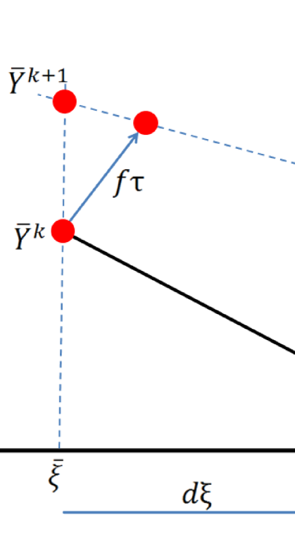
Figure 1: (Color online). Schematic representation of the basic idea behind the Relaxation Redistribution Method (RRM). In a small neighborhood of the pivot Y¯ksuperscript¯𝑌𝑘\bar{Y}^{k} (large circles), a linear approximation of the SIM at the iteration k𝑘k is considered. With the aim of driving the pivot towards the SIM, RRM [13, 12, 6] prescribes an updating rule Y¯kY¯k+1superscript¯𝑌𝑘superscript¯𝑌𝑘1\bar{Y}^{k}\rightarrow\bar{Y}^{k+1} as schematically sketched above (small circles represent neighbors of the pivot). Here, an ODEs system (21) whose dynamics approximates the latter updating rule is suggested and tested.

Let the dynamical system (1) be characterized by a hierarchy of time scales, and let τ𝜏\tau be of the order of the fastest scale of (1). Let the q×n𝑞𝑛q\times n matrix B𝐵B and its j𝑗j-th row Bjsubscript𝐵𝑗B_{j}

B=[b11b1nbq1bqn],Bj=[bj1,,bjn],formulae-sequence𝐵delimited-[]subscript𝑏11subscript𝑏1𝑛missing-subexpressionmissing-subexpressionmissing-subexpressionmissing-subexpressionmissing-subexpressionmissing-subexpressionmissing-subexpressionmissing-subexpressionmissing-subexpressionmissing-subexpressionmissing-subexpressionmissing-subexpressionmissing-subexpressionmissing-subexpressionmissing-subexpressionmissing-subexpressionmissing-subexpressionmissing-subexpressionmissing-subexpressionmissing-subexpressionmissing-subexpressionmissing-subexpressionmissing-subexpressionmissing-subexpressionmissing-subexpressionmissing-subexpressionmissing-subexpressionmissing-subexpressionmissing-subexpressionmissing-subexpressionmissing-subexpressionmissing-subexpressionmissing-subexpressionmissing-subexpressionsubscript𝑏𝑞1subscript𝑏𝑞𝑛missing-subexpressionmissing-subexpressionmissing-subexpressionmissing-subexpressionmissing-subexpressionmissing-subexpressionmissing-subexpressionmissing-subexpressionmissing-subexpressionmissing-subexpressionmissing-subexpressionmissing-subexpressionmissing-subexpressionmissing-subexpressionmissing-subexpressionmissing-subexpressionmissing-subexpressionsubscript𝐵𝑗subscript𝑏𝑗1subscript𝑏𝑗𝑛B=\left[{\begin{array}[]{*{20}c}{b_{11}}&\cdots&{b_{1n}}\\ \vdots&\ddots&\vdots\\ {b_{q1}}&\cdots&{b_{qn}}\\ \end{array}}\right],\;B_{j}=\left[{b_{j1},...,b_{jn}}\right], (6)

define a linear mapping from the phase-space U𝑈U into a reduced space ΞΞ\Xi of dimension q<<nmuch-less-than𝑞𝑛q<<n:

BY=ξ,ξ=[ξ1ξq]Ξ,formulae-sequence𝐵𝑌𝜉𝜉delimited-[]subscript𝜉1missing-subexpressionmissing-subexpressionmissing-subexpressionmissing-subexpressionmissing-subexpressionmissing-subexpressionmissing-subexpressionmissing-subexpressionmissing-subexpressionmissing-subexpressionmissing-subexpressionmissing-subexpressionmissing-subexpressionmissing-subexpressionmissing-subexpressionmissing-subexpressionmissing-subexpressionmissing-subexpressionmissing-subexpressionmissing-subexpressionmissing-subexpressionmissing-subexpressionmissing-subexpressionmissing-subexpressionmissing-subexpressionmissing-subexpressionmissing-subexpressionmissing-subexpressionmissing-subexpressionmissing-subexpressionmissing-subexpressionmissing-subexpressionmissing-subexpressionmissing-subexpressionmissing-subexpressionmissing-subexpressionmissing-subexpressionmissing-subexpressionsubscript𝜉𝑞missing-subexpressionmissing-subexpressionmissing-subexpressionmissing-subexpressionmissing-subexpressionmissing-subexpressionmissing-subexpressionmissing-subexpressionmissing-subexpressionmissing-subexpressionmissing-subexpressionmissing-subexpressionmissing-subexpressionmissing-subexpressionmissing-subexpressionmissing-subexpressionmissing-subexpressionmissing-subexpressionmissing-subexpressionΞBY=\xi,\quad\xi=\left[{\begin{array}[]{*{20}c}{\xi_{1}}\\ \vdots\\ {\xi_{q}}\\ \end{array}}\right]\in\Xi, (7)

such that a macrostate ξ𝜉\xi can be associated with any microstate Y𝑌Y via the (7). In the following, we develop an iterative methodology for refining an initial approximation of the SIM in a vicinity of a given macrostate ξ¯Ξ¯𝜉Ξ\bar{\xi}\in\Xi. To this end, at each iteration k𝑘k, we assume that, in a neighborhood of ξ¯¯𝜉\bar{\xi}, the SIM is approximated by an affine linear mapping, k:ΞU:superscript𝑘Ξ𝑈\mathcal{F}^{k}:\Xi\to U, of the form:

k:Y=Akξ+lk,k(ξ¯)=Y¯k,\mathcal{F}^{k}:\quad Y=A^{k}\xi+l^{k},\quad\mathcal{F}^{k}\left(\bar{\xi}\right)=\bar{Y}^{k}, (8)

where Aksuperscript𝐴𝑘A^{k} and lksuperscript𝑙𝑘l^{k} are a n×q𝑛𝑞n\times q matrix and a n×1𝑛1n\times 1 column vector, respectively, such that:

Ak=[a11ka1qkan1kanqk],Aik=[a1ikanik],lk=[l1klnk].formulae-sequencesuperscript𝐴𝑘delimited-[]superscriptsubscript𝑎11𝑘superscriptsubscript𝑎1𝑞𝑘missing-subexpressionmissing-subexpressionmissing-subexpressionmissing-subexpressionmissing-subexpressionmissing-subexpressionmissing-subexpressionmissing-subexpressionmissing-subexpressionmissing-subexpressionmissing-subexpressionmissing-subexpressionmissing-subexpressionmissing-subexpressionmissing-subexpressionmissing-subexpressionmissing-subexpressionmissing-subexpressionmissing-subexpressionmissing-subexpressionmissing-subexpressionmissing-subexpressionmissing-subexpressionmissing-subexpressionmissing-subexpressionmissing-subexpressionmissing-subexpressionmissing-subexpressionmissing-subexpressionmissing-subexpressionmissing-subexpressionmissing-subexpressionmissing-subexpressionmissing-subexpressionsuperscriptsubscript𝑎𝑛1𝑘superscriptsubscript𝑎𝑛𝑞𝑘missing-subexpressionmissing-subexpressionmissing-subexpressionmissing-subexpressionmissing-subexpressionmissing-subexpressionmissing-subexpressionmissing-subexpressionmissing-subexpressionmissing-subexpressionmissing-subexpressionmissing-subexpressionmissing-subexpressionmissing-subexpressionmissing-subexpressionmissing-subexpressionmissing-subexpressionformulae-sequencesuperscriptsubscript𝐴𝑖𝑘delimited-[]superscriptsubscript𝑎1𝑖𝑘missing-subexpressionmissing-subexpressionmissing-subexpressionmissing-subexpressionmissing-subexpressionmissing-subexpressionmissing-subexpressionmissing-subexpressionmissing-subexpressionmissing-subexpressionmissing-subexpressionmissing-subexpressionmissing-subexpressionmissing-subexpressionmissing-subexpressionmissing-subexpressionmissing-subexpressionmissing-subexpressionmissing-subexpressionmissing-subexpressionmissing-subexpressionmissing-subexpressionmissing-subexpressionmissing-subexpressionmissing-subexpressionmissing-subexpressionmissing-subexpressionmissing-subexpressionmissing-subexpressionmissing-subexpressionmissing-subexpressionmissing-subexpressionmissing-subexpressionmissing-subexpressionmissing-subexpressionmissing-subexpressionmissing-subexpressionmissing-subexpressionsuperscriptsubscript𝑎𝑛𝑖𝑘missing-subexpressionmissing-subexpressionmissing-subexpressionmissing-subexpressionmissing-subexpressionmissing-subexpressionmissing-subexpressionmissing-subexpressionmissing-subexpressionmissing-subexpressionmissing-subexpressionmissing-subexpressionmissing-subexpressionmissing-subexpressionmissing-subexpressionmissing-subexpressionmissing-subexpressionmissing-subexpressionmissing-subexpressionsuperscript𝑙𝑘delimited-[]superscriptsubscript𝑙1𝑘missing-subexpressionmissing-subexpressionmissing-subexpressionmissing-subexpressionmissing-subexpressionmissing-subexpressionmissing-subexpressionmissing-subexpressionmissing-subexpressionmissing-subexpressionmissing-subexpressionmissing-subexpressionmissing-subexpressionmissing-subexpressionmissing-subexpressionmissing-subexpressionmissing-subexpressionmissing-subexpressionmissing-subexpressionmissing-subexpressionmissing-subexpressionmissing-subexpressionmissing-subexpressionmissing-subexpressionmissing-subexpressionmissing-subexpressionmissing-subexpressionmissing-subexpressionmissing-subexpressionmissing-subexpressionmissing-subexpressionmissing-subexpressionmissing-subexpressionmissing-subexpressionmissing-subexpressionmissing-subexpressionmissing-subexpressionmissing-subexpressionsuperscriptsubscript𝑙𝑛𝑘missing-subexpressionmissing-subexpressionmissing-subexpressionmissing-subexpressionmissing-subexpressionmissing-subexpressionmissing-subexpressionmissing-subexpressionmissing-subexpressionmissing-subexpressionmissing-subexpressionmissing-subexpressionmissing-subexpressionmissing-subexpressionmissing-subexpressionmissing-subexpressionmissing-subexpressionmissing-subexpressionmissing-subexpressionA^{k}=\left[{\begin{array}[]{*{20}c}{a_{11}^{k}}&\cdots&{a_{1q}^{k}}\\ \vdots&\ddots&\vdots\\ {a_{n1}^{k}}&\cdots&{a_{nq}^{k}}\\ \end{array}}\right],\;A_{i}^{k}=\left[{\begin{array}[]{*{20}c}{a_{1i}^{k}}\\ \vdots\\ {a_{ni}^{k}}\\ \end{array}}\right],\;\;l^{k}=\left[{\begin{array}[]{*{20}c}{l_{1}^{k}}\\ \vdots\\ {l_{n}^{k}}\\ \end{array}}\right]. (9)

Notice that, the over-bar denotes the pivot (Y¯ksuperscript¯𝑌𝑘\bar{Y}^{k} in Fig. 1) at an arbitrary iteration k𝑘k along with the corresponding macrostate ξ¯¯𝜉\bar{\xi}.

For the state Y¯k=k(ξ¯)superscript¯𝑌𝑘superscript𝑘¯𝜉\bar{Y}^{k}=\mathcal{F}^{k}(\bar{\xi}) belongs to the space defined by the linear function in (8), the column vector lksuperscript𝑙𝑘l^{k} satisfies:

lk=Y¯kAkξ¯,ξ¯=BY¯k.formulae-sequencesuperscript𝑙𝑘superscript¯𝑌𝑘superscript𝐴𝑘¯𝜉¯𝜉𝐵superscript¯𝑌𝑘l^{k}=\bar{Y}^{k}-A^{k}\bar{\xi},\quad\bar{\xi}=B\bar{Y}^{k}.

Assuming the existence of a q𝑞q-dimensional SIM, ΩSIMsuperscriptΩ𝑆𝐼𝑀\Omega^{SIM}, we aim at devising a procedure for updating the linear mapping (8):

k+1:Y=Ak+1ξ+lk+1,\mathcal{F}^{k+1}:\quad Y=A^{k+1}\xi+l^{k+1}, (10)

such that (10) describes ΩSIMsuperscriptΩ𝑆𝐼𝑀\Omega^{SIM} with a better accuracy than (8) in a neighborhood of ξ¯¯𝜉\bar{\xi}. Toward this end, we follow the rationale behind the Relaxation Redistribution Method (RRM) introduced in [5, 12]. We stress that, at any iteration k𝑘k, the manifold is described by the mapping ksuperscript𝑘\mathcal{F}^{k} with the (q+1)𝑞1(q+1) microstates Y¯ksuperscript¯𝑌𝑘\bar{Y}^{k}, Y¯k+Aikdξsuperscript¯𝑌𝑘subscriptsuperscript𝐴𝑘𝑖𝑑𝜉\bar{Y}^{k}+A^{k}_{i}d\xi belonging to the affine subspace (8).

In Fig. 1, we pictorially show the relaxation of Y¯ksuperscript¯𝑌𝑘\bar{Y}^{k} (large circle) and one of its q𝑞q neighbors (small circle)

Y¯k+Aikdξ,i=1,,q,formulae-sequencesuperscript¯𝑌𝑘subscriptsuperscript𝐴𝑘𝑖𝑑𝜉𝑖1𝑞\bar{Y}^{k}+A^{k}_{i}d\xi,\quad i=1,...,q,

(all in the space defined by ksuperscript𝑘\mathcal{F}^{k}) toward ΩSIMsuperscriptΩ𝑆𝐼𝑀\Omega^{SIM} during the time τ𝜏\tau, where dξ𝑑𝜉d\xi is a small parameter. Notice that, owing to arbitrariness in picking the i𝑖i-th neighbor, for simplicity we make the choice dξi=dξ,i𝑑subscript𝜉𝑖𝑑𝜉for-all𝑖d\xi_{i}=d\xi,\;\forall i. According to the RRM algorithm [12], k+1superscript𝑘1\mathcal{F}^{k+1} describes the subspace defined by the set of q+1𝑞1q+1 relaxed states. The updated points can be written as:

Y¯k+f(Y¯k)τ,Y¯k+Aikdξ+f(Y¯k+Aikdξ)τ,i=1,,q,superscript¯𝑌𝑘𝑓superscript¯𝑌𝑘𝜏formulae-sequencesuperscript¯𝑌𝑘subscriptsuperscript𝐴𝑘𝑖𝑑𝜉𝑓superscript¯𝑌𝑘subscriptsuperscript𝐴𝑘𝑖𝑑𝜉𝜏𝑖1𝑞\begin{array}[]{l}\bar{Y}^{k}+f\left(\bar{Y}^{k}\right)\tau,\\ \bar{Y}^{k}+A^{k}_{i}d\xi+f\left(\bar{Y}^{k}+A^{k}_{i}d\xi\right)\tau,\quad i=1,...,q,\end{array} (11)

which represent the advance in time of the (q+1)𝑞1(q+1) points Y¯ksuperscript¯𝑌𝑘\bar{Y}^{k}, Y¯k+Aikdξsuperscript¯𝑌𝑘subscriptsuperscript𝐴𝑘𝑖𝑑𝜉\bar{Y}^{k}+A^{k}_{i}d\xi during a period τ𝜏\tau, according to an explicit Euler scheme. Upon linearization of the right-hand side of (1), f(Y+dY)f(Y)+J(Y)dY𝑓𝑌𝑑𝑌𝑓𝑌𝐽𝑌𝑑𝑌f\left(Y+dY\right)\approx f\left(Y\right)+J\left(Y\right)dY, (11) take the approximate form:

Y¯k+f(Y¯k)τ,Y¯k+Aikdξ+f(Y¯k)τ+J(Y¯k)Aikdξτ,i=1,,qsuperscript¯𝑌𝑘𝑓superscript¯𝑌𝑘𝜏formulae-sequencesuperscript¯𝑌𝑘subscriptsuperscript𝐴𝑘𝑖𝑑𝜉𝑓superscript¯𝑌𝑘𝜏𝐽superscript¯𝑌𝑘subscriptsuperscript𝐴𝑘𝑖𝑑𝜉𝜏𝑖1𝑞\begin{array}[]{l}\bar{Y}^{k}+f\left(\bar{Y}^{k}\right)\tau,\\ \bar{Y}^{k}+A^{k}_{i}d\xi+f\left(\bar{Y}^{k}\right)\tau+J\left(\bar{Y}^{k}\right)A^{k}_{i}d\xi\tau,\quad i=1,...,q\end{array} (12)

with J=J(Y¯k)=[fi/Yj]𝐽𝐽superscript¯𝑌𝑘delimited-[]subscript𝑓𝑖subscript𝑌𝑗J=J\left(\bar{Y}^{k}\right)=\left[\partial f_{i}/\partial Y_{j}\right] denoting the Jacobian matrix evaluated at Y¯ksuperscript¯𝑌𝑘\bar{Y}^{k}. Thus, a set of q𝑞q vectors spanning the linear space described by k+1superscript𝑘1\mathcal{F}^{k+1} reads as follows:

Aik+J(Y¯k)Aikτ,i=1,,q.formulae-sequencesuperscriptsubscript𝐴𝑖𝑘𝐽superscript¯𝑌𝑘superscriptsubscript𝐴𝑖𝑘𝜏𝑖1𝑞A_{i}^{k}+J\left(\bar{Y}^{k}\right)A_{i}^{k}\tau,\quad i=1,...,q. (13)

The RRM algorithm [12] introduces a fictitious dynamics such that an arbitrary state Y¯k=k(ξ¯)superscript¯𝑌𝑘superscript𝑘¯𝜉\bar{Y}^{k}=\mathcal{F}^{k}\left(\bar{\xi}\right) ”moves” to a new location:

Y¯k+1=k+1(ξ¯)=i=1qα¯i[Aik+J(Y¯k)Aikτ]+Y¯k+f(Y¯k)τ,superscript¯𝑌𝑘1superscript𝑘1¯𝜉superscriptsubscript𝑖1𝑞subscript¯𝛼𝑖delimited-[]superscriptsubscript𝐴𝑖𝑘𝐽superscript¯𝑌𝑘superscriptsubscript𝐴𝑖𝑘𝜏superscript¯𝑌𝑘𝑓superscript¯𝑌𝑘𝜏\bar{Y}^{k+1}=\mathcal{F}^{k+1}\left(\bar{\xi}\right)=\sum_{i=1}^{q}\bar{\alpha}_{i}\left[A_{i}^{k}+J\left(\bar{Y}^{k}\right)A_{i}^{k}\tau\right]+\bar{Y}^{k}+f\left(\bar{Y}^{k}\right)\tau, (14)

which obeys the relationship:

ξ¯j=BjY¯k=BjY¯k+1,j=1,,q.formulae-sequencesubscript¯𝜉𝑗subscript𝐵𝑗superscript¯𝑌𝑘subscript𝐵𝑗superscript¯𝑌𝑘1𝑗1𝑞\bar{\xi}_{j}=B_{j}\bar{Y}^{k}=B_{j}\bar{Y}^{k+1},\quad j=1,...,q. (15)

Equations (15) stipulate that the movement Y¯kY¯k+1superscript¯𝑌𝑘superscript¯𝑌𝑘1\bar{Y}^{k}\rightarrow\bar{Y}^{k+1} is orthogonal to the parameter space ΞΞ\Xi (see also Fig. 1) and, upon substitution of (14) in the (15), enable the explicit computation of the variables α¯isubscript¯𝛼𝑖\bar{\alpha}_{i} in (14) by solving the linear system:

[1+B1JA1kτB1JAqkτBqJA1kτ1+BqJAqkτ][α¯1α¯q]=τ[B1fBqf]delimited-[]1subscript𝐵1𝐽superscriptsubscript𝐴1𝑘𝜏subscript𝐵1𝐽superscriptsubscript𝐴𝑞𝑘𝜏missing-subexpressionmissing-subexpressionmissing-subexpressionmissing-subexpressionmissing-subexpressionmissing-subexpressionmissing-subexpressionmissing-subexpressionmissing-subexpressionmissing-subexpressionmissing-subexpressionmissing-subexpressionmissing-subexpressionmissing-subexpressionmissing-subexpressionmissing-subexpressionmissing-subexpressionmissing-subexpressionmissing-subexpressionmissing-subexpressionmissing-subexpressionmissing-subexpressionmissing-subexpressionmissing-subexpressionmissing-subexpressionmissing-subexpressionmissing-subexpressionmissing-subexpressionmissing-subexpressionmissing-subexpressionmissing-subexpressionmissing-subexpressionmissing-subexpressionmissing-subexpressionsubscript𝐵𝑞𝐽superscriptsubscript𝐴1𝑘𝜏1subscript𝐵𝑞𝐽superscriptsubscript𝐴𝑞𝑘𝜏missing-subexpressionmissing-subexpressionmissing-subexpressionmissing-subexpressionmissing-subexpressionmissing-subexpressionmissing-subexpressionmissing-subexpressionmissing-subexpressionmissing-subexpressionmissing-subexpressionmissing-subexpressionmissing-subexpressionmissing-subexpressionmissing-subexpressionmissing-subexpressionmissing-subexpressiondelimited-[]subscript¯𝛼1missing-subexpressionmissing-subexpressionmissing-subexpressionmissing-subexpressionmissing-subexpressionmissing-subexpressionmissing-subexpressionmissing-subexpressionmissing-subexpressionmissing-subexpressionmissing-subexpressionmissing-subexpressionmissing-subexpressionmissing-subexpressionmissing-subexpressionmissing-subexpressionmissing-subexpressionmissing-subexpressionmissing-subexpressionmissing-subexpressionmissing-subexpressionmissing-subexpressionmissing-subexpressionmissing-subexpressionmissing-subexpressionmissing-subexpressionmissing-subexpressionmissing-subexpressionmissing-subexpressionmissing-subexpressionmissing-subexpressionmissing-subexpressionmissing-subexpressionmissing-subexpressionmissing-subexpressionmissing-subexpressionmissing-subexpressionmissing-subexpressionsubscript¯𝛼𝑞missing-subexpressionmissing-subexpressionmissing-subexpressionmissing-subexpressionmissing-subexpressionmissing-subexpressionmissing-subexpressionmissing-subexpressionmissing-subexpressionmissing-subexpressionmissing-subexpressionmissing-subexpressionmissing-subexpressionmissing-subexpressionmissing-subexpressionmissing-subexpressionmissing-subexpressionmissing-subexpressionmissing-subexpression𝜏delimited-[]subscript𝐵1𝑓missing-subexpressionmissing-subexpressionmissing-subexpressionmissing-subexpressionmissing-subexpressionmissing-subexpressionmissing-subexpressionmissing-subexpressionmissing-subexpressionmissing-subexpressionmissing-subexpressionmissing-subexpressionmissing-subexpressionmissing-subexpressionmissing-subexpressionmissing-subexpressionmissing-subexpressionmissing-subexpressionmissing-subexpressionmissing-subexpressionmissing-subexpressionmissing-subexpressionmissing-subexpressionmissing-subexpressionmissing-subexpressionmissing-subexpressionmissing-subexpressionmissing-subexpressionmissing-subexpressionmissing-subexpressionmissing-subexpressionmissing-subexpressionmissing-subexpressionmissing-subexpressionmissing-subexpressionmissing-subexpressionmissing-subexpressionmissing-subexpressionsubscript𝐵𝑞𝑓missing-subexpressionmissing-subexpressionmissing-subexpressionmissing-subexpressionmissing-subexpressionmissing-subexpressionmissing-subexpressionmissing-subexpressionmissing-subexpressionmissing-subexpressionmissing-subexpressionmissing-subexpressionmissing-subexpressionmissing-subexpressionmissing-subexpressionmissing-subexpressionmissing-subexpressionmissing-subexpressionmissing-subexpression\left[{\begin{array}[]{*{20}c}{1+B_{1}JA_{1}^{k}\tau}&\cdots&{B_{1}JA_{q}^{k}\tau}\\ \vdots&\ddots&\vdots\\ {B_{q}JA_{1}^{k}\tau}&\cdots&{1+B_{q}JA_{q}^{k}\tau}\\ \end{array}}\right]\cdot\left[{\begin{array}[]{*{20}c}{\bar{\alpha}_{1}}\\ \vdots\\ {\bar{\alpha}_{q}}\\ \end{array}}\right]=-\tau\left[{\begin{array}[]{*{20}c}{B_{1}f}\\ \vdots\\ {B_{q}f}\\ \end{array}}\right] (16)

where due to (7) and (8) BiAjk=δijksubscript𝐵𝑖superscriptsubscript𝐴𝑗𝑘subscript𝛿𝑖𝑗for-all𝑘B_{i}A_{j}^{k}=\delta_{ij}\;\forall k, with δijsubscript𝛿𝑖𝑗\delta_{ij} being the Kronecker delta.In the following, in order to save notation, we assume that both the vector field f𝑓f and the Jacobian matrix J𝐽J are computed at Y¯ksuperscript¯𝑌𝑘\bar{Y}^{k}; equation (14) takes the more compact form:

Y¯k+1=Y¯k+(fMkΦk1Bf)τ,superscript¯𝑌𝑘1superscript¯𝑌𝑘𝑓superscript𝑀𝑘subscriptsuperscriptΦ1𝑘𝐵𝑓𝜏\bar{Y}^{k+1}=\bar{Y}^{k}+\left(f-M^{k}\Phi^{-1}_{k}Bf\right)\tau, (17)

with ΦksubscriptΦ𝑘\Phi_{k} denoting the q×q𝑞𝑞q\times q matrix on the left-hand side of (16), whereas Mksuperscript𝑀𝑘M^{k} is a n×q𝑛𝑞n\times q column matrix defined as follows:

Mk=[A1k+JA1kτ,,Aqk+JAqkτ]=(I+Jτ)Ak,superscript𝑀𝑘superscriptsubscript𝐴1𝑘𝐽superscriptsubscript𝐴1𝑘𝜏superscriptsubscript𝐴𝑞𝑘𝐽superscriptsubscript𝐴𝑞𝑘𝜏𝐼𝐽𝜏superscript𝐴𝑘M^{k}=\left[{A_{1}^{k}+JA_{1}^{k}\tau},...,{A_{q}^{k}+JA_{q}^{k}\tau}\right]=\left(I+J\tau\right)A^{k},

with I denoting the n×n𝑛𝑛n\times n unit matrix. It is worth stressing that the solution of the equations (17) requires an updating rule for the matrix A𝐴A in (9) as well: AkAk+1superscript𝐴𝑘superscript𝐴𝑘1A^{k}\rightarrow A^{k+1}. For this purpose, we notice that an arbitrary point Y𝑌Y in the linear space described by the function k+1superscript𝑘1\mathcal{F}^{k+1} takes the form

k+1:Y=i=1qαi(Aik+JAikτ)+Y¯k+1,\mathcal{F}^{k+1}:\quad Y=\sum_{i=1}^{q}\alpha_{i}\left(A_{i}^{k}+JA_{i}^{k}\tau\right)+\bar{Y}^{k+1}, (18)

hence the j𝑗j-th parameter ξjsubscript𝜉𝑗\xi_{j} corresponding to Y𝑌Y is

ξj=i=1qαi(δij+BjJAikτ)+ξ¯j,subscript𝜉𝑗superscriptsubscript𝑖1𝑞subscript𝛼𝑖subscript𝛿𝑖𝑗subscript𝐵𝑗𝐽superscriptsubscript𝐴𝑖𝑘𝜏subscript¯𝜉𝑗\xi_{j}=\sum_{i=1}^{q}\alpha_{i}\left(\delta_{ij}+B_{j}JA_{i}^{k}\tau\right)+\bar{\xi}_{j},

or, equivalently, in matrix notation:

Y=MkΛ+Y¯k+1,ξ=ΦkΛ+ξ¯,formulae-sequence𝑌superscript𝑀𝑘Λsuperscript¯𝑌𝑘1𝜉subscriptΦ𝑘Λ¯𝜉Y=M^{k}\Lambda+\bar{Y}^{k+1},\quad\xi=\Phi_{k}\Lambda+\bar{\xi}, (19)

with Λ=[α1,,αq]TΛsuperscriptsubscript𝛼1subscript𝛼𝑞𝑇\Lambda=\left[\alpha_{1},...,\alpha_{q}\right]^{T}. Equation (18) stems from (14) where the origin, Y¯k+f(Y¯k)τsuperscript¯𝑌𝑘𝑓superscript¯𝑌𝑘𝜏\bar{Y}^{k}+f(\bar{Y}^{k})\tau, of the affine subspace has been replaced with Y¯k+1superscript¯𝑌𝑘1\bar{Y}^{k+1}.

Equations (19) yield the function k+1superscript𝑘1\mathcal{F}^{k+1} in the form (10):

Y=MkΦk1(ξξ¯)+Y¯k+1,𝑌superscript𝑀𝑘subscriptsuperscriptΦ1𝑘𝜉¯𝜉superscript¯𝑌𝑘1Y=M^{k}\Phi^{-1}_{k}\left(\xi-\bar{\xi}\right)+\bar{Y}^{k+1},

where

Ak+1=MkΦk1,lk+1=Y¯k+1MkΦk1ξ¯.formulae-sequencesuperscript𝐴𝑘1superscript𝑀𝑘subscriptsuperscriptΦ1𝑘superscript𝑙𝑘1superscript¯𝑌𝑘1superscript𝑀𝑘subscriptsuperscriptΦ1𝑘¯𝜉A^{k+1}=M^{k}\Phi^{-1}_{k},\quad l^{k+1}=\bar{Y}^{k+1}-M^{k}\Phi^{-1}_{k}\bar{\xi}. (20)

The updating rules (17) and (20) can be interpreted as the explicit Euler numerical scheme for solving the following dynamical system:

dYdt=fMΦ1Bf,dAdt=[MΦ1A]τ1.formulae-sequence𝑑𝑌𝑑𝑡𝑓𝑀superscriptΦ1𝐵𝑓𝑑𝐴𝑑𝑡delimited-[]𝑀superscriptΦ1𝐴superscript𝜏1\frac{{dY}}{{dt}}=f-M\Phi^{-1}Bf,\quad\frac{dA}{dt}=\left[M\Phi^{-1}-A\right]\tau^{-1}. (21)

The second equation in (21) can be derived, by analogy with (17), after recasting the first equation in (20) as follows:

Ak+1=Ak+[(MkΦk1Ak)τ1]τ.superscript𝐴𝑘1superscript𝐴𝑘delimited-[]superscript𝑀𝑘subscriptsuperscriptΦ1𝑘superscript𝐴𝑘superscript𝜏1𝜏A^{k+1}=A^{k}+\left[\left(M^{k}\Phi^{-1}_{k}-A^{k}\right)\tau^{-1}\right]\tau.

The above equations (21) are the governing equations of the linearized RRM, which dictate a fictitious temporal evolution of a state Y𝑌Y and a n×q𝑛𝑞n\times q matrix A𝐴A

A=[A1,,Aq],Ai=[a1iani],formulae-sequence𝐴subscript𝐴1subscript𝐴𝑞subscript𝐴𝑖delimited-[]subscript𝑎1𝑖missing-subexpressionmissing-subexpressionmissing-subexpressionmissing-subexpressionmissing-subexpressionmissing-subexpressionmissing-subexpressionmissing-subexpressionmissing-subexpressionmissing-subexpressionmissing-subexpressionmissing-subexpressionmissing-subexpressionmissing-subexpressionmissing-subexpressionmissing-subexpressionmissing-subexpressionmissing-subexpressionmissing-subexpressionmissing-subexpressionmissing-subexpressionmissing-subexpressionmissing-subexpressionmissing-subexpressionmissing-subexpressionmissing-subexpressionmissing-subexpressionmissing-subexpressionmissing-subexpressionmissing-subexpressionmissing-subexpressionmissing-subexpressionmissing-subexpressionmissing-subexpressionmissing-subexpressionmissing-subexpressionmissing-subexpressionmissing-subexpressionsubscript𝑎𝑛𝑖missing-subexpressionmissing-subexpressionmissing-subexpressionmissing-subexpressionmissing-subexpressionmissing-subexpressionmissing-subexpressionmissing-subexpressionmissing-subexpressionmissing-subexpressionmissing-subexpressionmissing-subexpressionmissing-subexpressionmissing-subexpressionmissing-subexpressionmissing-subexpressionmissing-subexpressionmissing-subexpressionmissing-subexpressionA=\left[A_{1},...,A_{q}\right],\quad A_{i}=\left[{\begin{array}[]{*{20}c}{a_{1i}}\\ \vdots\\ {a_{ni}}\\ \end{array}}\right],

(defining an affine linear mapping of the form ::absent\mathcal{F}: Y=Aξ+l𝑌𝐴𝜉𝑙Y=A\xi+l) towards the corresponding q𝑞q-dimensional slow invariant manifold ΩSIMsuperscriptΩ𝑆𝐼𝑀\Omega^{SIM} in a neighborhood of a given macroscopic state ξ¯¯𝜉\bar{\xi}, with

M=[A1+JA1τ,,Aq+JAqτ],Φ(i,j)=δij+BiJAjτ.formulae-sequence𝑀subscript𝐴1𝐽subscript𝐴1𝜏subscript𝐴𝑞𝐽subscript𝐴𝑞𝜏Φ𝑖𝑗subscript𝛿𝑖𝑗subscript𝐵𝑖𝐽subscript𝐴𝑗𝜏M=\left[{A_{1}+JA_{1}\tau},...,{A_{q}+JA_{q}\tau}\right],\;\Phi(i,j)=\delta_{ij}+B_{i}JA_{j}\tau.

For the sake of clarity, we point out that the dynamics (21) (as well as the RRM dynamics in [12]) is referred to as fictitious because, unlike the original detailed system (1), no physical or chemical processes are typically described by it.

Moreover, we stress that the presence of the time-scale τ𝜏\tau in the right-hand side of the equations in (21) introduces a remarkable stiffness, thus the ODEs (21) typically require state of the art stiff integrators (see, e.g., [42]). According to the RRM method, the SIM is obtained when the relaxation and redistribution steps balance each other (details can be found in [12]). In the suggested algorithm, the analogous condition is satisfied at the steady state (here denoted as Y=Yss𝑌superscript𝑌𝑠𝑠Y=Y^{ss} and A=Ass𝐴superscript𝐴𝑠𝑠A=A^{ss}) of the dynamical system (21). Hence, the SIM is given (in a vicinity of ξ¯¯𝜉\bar{\xi}) by:

ΩSIM:Y=Assξ+lss,lss=YssAssξ¯.\Omega^{SIM}:\quad Y=A^{ss}\xi+l^{ss},\quad l^{ss}=Y^{ss}-A^{ss}\bar{\xi}. (22)

We stress that computation of the quantity lsssuperscript𝑙𝑠𝑠l^{ss} does not require additional refinements, and it is performed by (22) (upon convergence of (21)) if a linear approximation is to be provided for approximating the mapping (3) in a neighborhood of Ysssuperscript𝑌𝑠𝑠Y^{ss}.

It is worth noticing that, inspection of the right-hand side of the first equation in (21) reveals a clear connection between the RRM method introduced in [13, 12] and the film equation (5). In fact, although (21) represents a system of ordinary differential equations whereas (5) is a partial differential equation, the former only describes the (5) locally in a vicinity of a macrostate ξ¯¯𝜉\bar{\xi}. In this respect, the projector onto the tangent space of a manifold ΩΩ\Omega takes the explicit form: P=MΦ1B𝑃𝑀superscriptΦ1𝐵P=M\Phi^{-1}B. In this respect, the latter operator satisfies the condition of projectors:

P2=MΦ1BMΦ1B=MΦ1B=P,superscript𝑃2𝑀superscriptΦ1𝐵𝑀superscriptΦ1𝐵𝑀superscriptΦ1𝐵𝑃P^{2}=M\Phi^{-1}BM\Phi^{-1}B=M\Phi^{-1}B=P,

due to the relation BM=Φ𝐵𝑀ΦBM=\Phi. Similarly to (5), the governing equations of the linearized RRM (21) prescribe a composition of two motions: the first one along the detailed dynamics f𝑓f, while the second one along the tangent space of ΩΩ\Omega, Pf=MΦ1Bf𝑃𝑓𝑀superscriptΦ1𝐵𝑓-Pf=-M\Phi^{-1}Bf. Finally, at steady state of (21), the invariance condition (4) is satisfied:

fMΦ1Bf=(IMΦ1B)f=(IP)f=0.𝑓𝑀superscriptΦ1𝐵𝑓𝐼𝑀superscriptΦ1𝐵𝑓𝐼𝑃𝑓0f-M\Phi^{-1}Bf=\left(I-M\Phi^{-1}B\right)f=\left(I-P\right)f=0.

The above equation imposes that, on the SIM, the component of dynamics f𝑓f in the fast subspace vanishes. Since that condition lies at the heart of other popular methods (such as ILDM and CSP [38, 29]), this explains the formal resemblance of (21) (at steady state) to the equations adopted in ILDM and CSP.

3.2 Fast subspace

The methodology proposed in the previous section can be utilized for extracting the slow invariant manifold (i.e. the subspace of slow motions or slow subspace, for short) with respect to the ODE system (1). Nevertheless, this is only one aspect of model reduction: Computing the fast subspace is indeed required in order to achieve the complete decomposition of the full dynamics f𝑓f (slow-fast decomposition).

We notice that, towards this end, several approaches have been proposed in the literature. For instance, the notion of thermodynamic projector [18, 9, 8] for dissipative systems supported by a thermodynamic Lyapunov function, the spectral decomposition of the Jacobian matrix J𝐽J [38], and the CSP algorithm [22] are some of the most popular examples.

Those methods might be adopted in combination with the above technique (21) as well, for an a posteriori reconstruction of the fast subspace. However, here in the same spirit of the method presented in section 3.1, we propose an alternative procedure for computing the fast subspace, in a neighborhood of a given macrostate ξ¯¯𝜉\bar{\xi}, once the linear function (22) has been computed.
Refer to caption
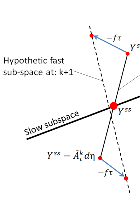
Figure 2: (Color online). Rationale behind the refinement process of the fast subspace: In a neighborhood of the SIM (slow subspace), the anti-parallel dynamics f𝑓-f reacts with a torque if (25) does not span the fast subspace. As a result, the latter subspace is the stable stationary solution of Eqs. (30) and (31). Small circles denote neighbors of a pivot (large circle).

Let us assume that the fast subspace can be uniquely parameterized (at least locally) by the variables ηi,i=1,,nqrformulae-sequencesubscript𝜂𝑖𝑖1𝑛𝑞𝑟\eta_{i},\;i=1,...,n-q-r. Let the z×n𝑧𝑛z\times n matrix B~~𝐵\tilde{B} and its j𝑗j-th row B~jsubscript~𝐵𝑗\tilde{B}_{j}

B~=[b11b1nbz1bzn],B~j=[bj1,,bjn],z=nqr,formulae-sequence~𝐵delimited-[]subscript𝑏11subscript𝑏1𝑛missing-subexpressionmissing-subexpressionmissing-subexpressionmissing-subexpressionmissing-subexpressionmissing-subexpressionmissing-subexpressionmissing-subexpressionmissing-subexpressionmissing-subexpressionmissing-subexpressionmissing-subexpressionmissing-subexpressionmissing-subexpressionmissing-subexpressionmissing-subexpressionmissing-subexpressionmissing-subexpressionmissing-subexpressionmissing-subexpressionmissing-subexpressionmissing-subexpressionmissing-subexpressionmissing-subexpressionmissing-subexpressionmissing-subexpressionmissing-subexpressionmissing-subexpressionmissing-subexpressionmissing-subexpressionmissing-subexpressionmissing-subexpressionmissing-subexpressionmissing-subexpressionsubscript𝑏𝑧1subscript𝑏𝑧𝑛missing-subexpressionmissing-subexpressionmissing-subexpressionmissing-subexpressionmissing-subexpressionmissing-subexpressionmissing-subexpressionmissing-subexpressionmissing-subexpressionmissing-subexpressionmissing-subexpressionmissing-subexpressionmissing-subexpressionmissing-subexpressionmissing-subexpressionmissing-subexpressionmissing-subexpressionformulae-sequencesubscript~𝐵𝑗subscript𝑏𝑗1subscript𝑏𝑗𝑛𝑧𝑛𝑞𝑟\tilde{B}=\left[{\begin{array}[]{*{20}c}{b_{11}}&\cdots&{b_{1n}}\\ \vdots&\ddots&\vdots\\ {b_{z1}}&\cdots&{b_{zn}}\\ \end{array}}\right],\;\tilde{B}_{j}=\left[{b_{j1},...,b_{jn}}\right],\quad z=n-q-r, (23)

define a linear mapping:

B~Y=η,η=[η1ηz],formulae-sequence~𝐵𝑌𝜂𝜂delimited-[]subscript𝜂1missing-subexpressionmissing-subexpressionmissing-subexpressionmissing-subexpressionmissing-subexpressionmissing-subexpressionmissing-subexpressionmissing-subexpressionmissing-subexpressionmissing-subexpressionmissing-subexpressionmissing-subexpressionmissing-subexpressionmissing-subexpressionmissing-subexpressionmissing-subexpressionmissing-subexpressionmissing-subexpressionmissing-subexpressionmissing-subexpressionmissing-subexpressionmissing-subexpressionmissing-subexpressionmissing-subexpressionmissing-subexpressionmissing-subexpressionmissing-subexpressionmissing-subexpressionmissing-subexpressionmissing-subexpressionmissing-subexpressionmissing-subexpressionmissing-subexpressionmissing-subexpressionmissing-subexpressionmissing-subexpressionmissing-subexpressionmissing-subexpressionsubscript𝜂𝑧missing-subexpressionmissing-subexpressionmissing-subexpressionmissing-subexpressionmissing-subexpressionmissing-subexpressionmissing-subexpressionmissing-subexpressionmissing-subexpressionmissing-subexpressionmissing-subexpressionmissing-subexpressionmissing-subexpressionmissing-subexpressionmissing-subexpressionmissing-subexpressionmissing-subexpressionmissing-subexpressionmissing-subexpression\tilde{B}Y=\eta,\quad\eta=\left[{\begin{array}[]{*{20}c}{\eta_{1}}\\ \vdots\\ {\eta_{z}}\\ \end{array}}\right], (24)

where the dynamics f𝑓f of the system (1) obeys a set of r𝑟r linear conservation laws. In a neighborhood of the SIM point Ysssuperscript𝑌𝑠𝑠Y^{ss}, at a given iteration k𝑘k, the fast sub-space can be represented by a linear function as follows:

Y=A~kη+l~k,𝑌superscript~𝐴𝑘𝜂superscript~𝑙𝑘Y=\tilde{A}^{k}\eta+\tilde{l}^{k}, (25)

with

A~k=[a~11ka~1zka~n1ka~nzk],A~ik=[a~1ika~nik],l~k=[l~1kl~nk].formulae-sequencesuperscript~𝐴𝑘delimited-[]superscriptsubscript~𝑎11𝑘superscriptsubscript~𝑎1𝑧𝑘missing-subexpressionmissing-subexpressionmissing-subexpressionmissing-subexpressionmissing-subexpressionmissing-subexpressionmissing-subexpressionmissing-subexpressionmissing-subexpressionmissing-subexpressionmissing-subexpressionmissing-subexpressionmissing-subexpressionmissing-subexpressionmissing-subexpressionmissing-subexpressionmissing-subexpressionmissing-subexpressionmissing-subexpressionmissing-subexpressionmissing-subexpressionmissing-subexpressionmissing-subexpressionmissing-subexpressionmissing-subexpressionmissing-subexpressionmissing-subexpressionmissing-subexpressionmissing-subexpressionmissing-subexpressionmissing-subexpressionmissing-subexpressionmissing-subexpressionmissing-subexpressionsuperscriptsubscript~𝑎𝑛1𝑘superscriptsubscript~𝑎𝑛𝑧𝑘missing-subexpressionmissing-subexpressionmissing-subexpressionmissing-subexpressionmissing-subexpressionmissing-subexpressionmissing-subexpressionmissing-subexpressionmissing-subexpressionmissing-subexpressionmissing-subexpressionmissing-subexpressionmissing-subexpressionmissing-subexpressionmissing-subexpressionmissing-subexpressionmissing-subexpressionformulae-sequencesuperscriptsubscript~𝐴𝑖𝑘delimited-[]superscriptsubscript~𝑎1𝑖𝑘missing-subexpressionmissing-subexpressionmissing-subexpressionmissing-subexpressionmissing-subexpressionmissing-subexpressionmissing-subexpressionmissing-subexpressionmissing-subexpressionmissing-subexpressionmissing-subexpressionmissing-subexpressionmissing-subexpressionmissing-subexpressionmissing-subexpressionmissing-subexpressionmissing-subexpressionmissing-subexpressionmissing-subexpressionmissing-subexpressionmissing-subexpressionmissing-subexpressionmissing-subexpressionmissing-subexpressionmissing-subexpressionmissing-subexpressionmissing-subexpressionmissing-subexpressionmissing-subexpressionmissing-subexpressionmissing-subexpressionmissing-subexpressionmissing-subexpressionmissing-subexpressionmissing-subexpressionmissing-subexpressionmissing-subexpressionmissing-subexpressionsuperscriptsubscript~𝑎𝑛𝑖𝑘missing-subexpressionmissing-subexpressionmissing-subexpressionmissing-subexpressionmissing-subexpressionmissing-subexpressionmissing-subexpressionmissing-subexpressionmissing-subexpressionmissing-subexpressionmissing-subexpressionmissing-subexpressionmissing-subexpressionmissing-subexpressionmissing-subexpressionmissing-subexpressionmissing-subexpressionmissing-subexpressionmissing-subexpressionsuperscript~𝑙𝑘delimited-[]superscriptsubscript~𝑙1𝑘missing-subexpressionmissing-subexpressionmissing-subexpressionmissing-subexpressionmissing-subexpressionmissing-subexpressionmissing-subexpressionmissing-subexpressionmissing-subexpressionmissing-subexpressionmissing-subexpressionmissing-subexpressionmissing-subexpressionmissing-subexpressionmissing-subexpressionmissing-subexpressionmissing-subexpressionmissing-subexpressionmissing-subexpressionmissing-subexpressionmissing-subexpressionmissing-subexpressionmissing-subexpressionmissing-subexpressionmissing-subexpressionmissing-subexpressionmissing-subexpressionmissing-subexpressionmissing-subexpressionmissing-subexpressionmissing-subexpressionmissing-subexpressionmissing-subexpressionmissing-subexpressionmissing-subexpressionmissing-subexpressionmissing-subexpressionmissing-subexpressionsuperscriptsubscript~𝑙𝑛𝑘missing-subexpressionmissing-subexpressionmissing-subexpressionmissing-subexpressionmissing-subexpressionmissing-subexpressionmissing-subexpressionmissing-subexpressionmissing-subexpressionmissing-subexpressionmissing-subexpressionmissing-subexpressionmissing-subexpressionmissing-subexpressionmissing-subexpressionmissing-subexpressionmissing-subexpressionmissing-subexpressionmissing-subexpression\tilde{A}^{k}=\left[{\begin{array}[]{*{20}c}{\tilde{a}_{11}^{k}}&\cdots&{\tilde{a}_{1z}^{k}}\\ \vdots&\ddots&\vdots\\ {\tilde{a}_{n1}^{k}}&\cdots&{\tilde{a}_{nz}^{k}}\\ \end{array}}\right],\;\tilde{A}_{i}^{k}=\left[{\begin{array}[]{*{20}c}{\tilde{a}_{1i}^{k}}\\ \vdots\\ {\tilde{a}_{ni}^{k}}\\ \end{array}}\right],\;\;\tilde{l}^{k}=\left[{\begin{array}[]{*{20}c}{\tilde{l}_{1}^{k}}\\ \vdots\\ {\tilde{l}_{n}^{k}}\\ \end{array}}\right]. (26)

Similarly to the procedure of section 3.1, here we aim at devising an iterative procedure

A~kA~k+1,l~kl~k+1,formulae-sequencesuperscript~𝐴𝑘superscript~𝐴𝑘1superscript~𝑙𝑘superscript~𝑙𝑘1\tilde{A}^{k}\rightarrow\tilde{A}^{k+1},\;\tilde{l}^{k}\rightarrow\tilde{l}^{k+1},

so that the function (25), in the limit k𝑘k\rightarrow\infty, accurately describes the fast subspace. Let dη𝑑𝜂d\eta denote an arbitrary small parameter. Following the pictorial representation of Fig. 2, for every variable ηisubscript𝜂𝑖\eta_{i} we consider the relaxation of the two neighbors (in the affine space (25)) of Ysssuperscript𝑌𝑠𝑠Y^{ss}

Yss+A~ikdη,YssA~ikdη,superscript𝑌𝑠𝑠superscriptsubscript~𝐴𝑖𝑘𝑑𝜂superscript𝑌𝑠𝑠superscriptsubscript~𝐴𝑖𝑘𝑑𝜂Y^{ss}+\tilde{A}_{i}^{k}d\eta,\;Y^{ss}-\tilde{A}_{i}^{k}d\eta,

under the anti-parallel dynamics f𝑓-f. After time τ𝜏\tau, these states move to the new locations:

Yss+A~ikdηf(Yss+A~ikdη)τ,YssA~ikdηf(YssA~ikdη)τ,superscript𝑌𝑠𝑠superscriptsubscript~𝐴𝑖𝑘𝑑𝜂𝑓superscript𝑌𝑠𝑠superscriptsubscript~𝐴𝑖𝑘𝑑𝜂𝜏superscript𝑌𝑠𝑠superscriptsubscript~𝐴𝑖𝑘𝑑𝜂𝑓superscript𝑌𝑠𝑠superscriptsubscript~𝐴𝑖𝑘𝑑𝜂𝜏Y^{ss}+\tilde{A}_{i}^{k}d\eta-f\left(Y^{ss}+\tilde{A}_{i}^{k}d\eta\right)\tau,\;Y^{ss}-\tilde{A}_{i}^{k}d\eta-f\left(Y^{ss}-\tilde{A}_{i}^{k}d\eta\right)\tau,

which, upon linearization of the vector field f𝑓f, take the approximate form:

Yss+A~ikdηf(Yss)τJ(Yss)A~ikdητ,YssA~ikdηf(Yss)τ+J(Yss)A~ikdητ.superscript𝑌𝑠𝑠superscriptsubscript~𝐴𝑖𝑘𝑑𝜂𝑓superscript𝑌𝑠𝑠𝜏𝐽superscript𝑌𝑠𝑠superscriptsubscript~𝐴𝑖𝑘𝑑𝜂𝜏superscript𝑌𝑠𝑠superscriptsubscript~𝐴𝑖𝑘𝑑𝜂𝑓superscript𝑌𝑠𝑠𝜏𝐽superscript𝑌𝑠𝑠superscriptsubscript~𝐴𝑖𝑘𝑑𝜂𝜏Y^{ss}+\tilde{A}_{i}^{k}d\eta-f\left(Y^{ss}\right)\tau-J\left(Y^{ss}\right)\tilde{A}_{i}^{k}d\eta\tau,\;Y^{ss}-\tilde{A}_{i}^{k}d\eta-f\left(Y^{ss}\right)\tau+J\left(Y^{ss}\right)\tilde{A}_{i}^{k}d\eta\tau.

Therefore, a set of z𝑧z vectors spanning the fast sub-space at the iteration k+1𝑘1k+1 reads:

A~ikJssA~ikτ,i=1,,z,formulae-sequencesuperscriptsubscript~𝐴𝑖𝑘superscript𝐽𝑠𝑠superscriptsubscript~𝐴𝑖𝑘𝜏𝑖1𝑧\tilde{A}_{i}^{k}-J^{ss}\tilde{A}_{i}^{k}\tau,\quad i=1,...,z,

where, for the sake of notations, Jss=J(Yss)superscript𝐽𝑠𝑠𝐽superscript𝑌𝑠𝑠J^{ss}=J\left(Y^{ss}\right). We can thus describe the updated fast sub-space as follows:

YYss=i=1zα~i(A~ikJssA~ikτ),𝑌superscript𝑌𝑠𝑠superscriptsubscript𝑖1𝑧subscript~𝛼𝑖superscriptsubscript~𝐴𝑖𝑘superscript𝐽𝑠𝑠superscriptsubscript~𝐴𝑖𝑘𝜏Y-Y^{ss}=\sum_{i=1}^{z}\tilde{\alpha}_{i}\left(\tilde{A}_{i}^{k}-J^{ss}\tilde{A}_{i}^{k}\tau\right),

or equivalently in matrix notations

YYss=M~kΛ~,𝑌superscript𝑌𝑠𝑠superscript~𝑀𝑘~ΛY-Y^{ss}=\tilde{M}^{k}\tilde{\Lambda}, (27)

with

M~k=[A~1kJssA~1kτ,,A~zkJssA~zkτ],Λ~=[α~1,,α~z]T.formulae-sequencesuperscript~𝑀𝑘superscriptsubscript~𝐴1𝑘superscript𝐽𝑠𝑠superscriptsubscript~𝐴1𝑘𝜏superscriptsubscript~𝐴𝑧𝑘superscript𝐽𝑠𝑠superscriptsubscript~𝐴𝑧𝑘𝜏~Λsuperscriptsubscript~𝛼1subscript~𝛼𝑧𝑇\tilde{M}^{k}=\left[{\tilde{A}_{1}^{k}-J^{ss}\tilde{A}_{1}^{k}\tau},...,{\tilde{A}_{z}^{k}-J^{ss}\tilde{A}_{z}^{k}\tau}\right],\tilde{\Lambda}=\left[\tilde{\alpha}_{1},...,\tilde{\alpha}_{z}\right]^{T}. (28)

By substituting the (27) into (24),

ηB~Yss=Φ~kΛ~,𝜂~𝐵superscript𝑌𝑠𝑠subscript~Φ𝑘~Λ\eta-\tilde{B}Y^{ss}=\tilde{\Phi}_{k}\tilde{\Lambda}, (29)

where the generic element Φ~k(i,j)subscript~Φ𝑘𝑖𝑗\tilde{\Phi}_{k}\left(i,j\right) of the z×z𝑧𝑧z\times z matrix Φ~ksubscript~Φ𝑘\tilde{\Phi}_{k} reads

Φ~k(i,j)=δijB~iJssA~jkτ,subscript~Φ𝑘𝑖𝑗subscript𝛿𝑖𝑗subscript~𝐵𝑖superscript𝐽𝑠𝑠superscriptsubscript~𝐴𝑗𝑘𝜏\tilde{\Phi}_{k}\left(i,j\right)=\delta_{ij}-\tilde{B}_{i}J^{ss}\tilde{A}_{j}^{k}\tau,

where, owing to (24) and (25), B~iA~jk=δijk.subscript~𝐵𝑖superscriptsubscript~𝐴𝑗𝑘subscript𝛿𝑖𝑗for-all𝑘\tilde{B}_{i}\tilde{A}_{j}^{k}=\delta_{ij}\;\forall k. From (27) and (29), it follows that at the iteration k+1𝑘1k+1 the linear function describing the fast sub-space is:

Y=M~Φ~k1(ηB~Yss)+Yss,𝑌~𝑀superscriptsubscript~Φ𝑘1𝜂~𝐵superscript𝑌𝑠𝑠superscript𝑌𝑠𝑠Y=\tilde{M}\tilde{\Phi}_{k}^{-1}\left(\eta-\tilde{B}Y^{ss}\right)+Y^{ss},

so that

A~k+1=M~kΦ~k1.superscript~𝐴𝑘1superscript~𝑀𝑘superscriptsubscript~Φ𝑘1\tilde{A}^{k+1}=\tilde{M}^{k}\tilde{\Phi}_{k}^{-1}. (30)

Similarly to the (20), the updating rule (30) can be regarded as the explicit Euler scheme for integrating the dynamical system:

dA~dt=[M~Φ~1A~]τ1,𝑑~𝐴𝑑𝑡delimited-[]~𝑀superscript~Φ1~𝐴superscript𝜏1\frac{d\tilde{A}}{dt}=\left[\tilde{M}\tilde{\Phi}^{-1}-\tilde{A}\right]\tau^{-1}, (31)

with

M~=[A~1JssA~1τ,,A~zJssA~zτ],Φ~(i,j)=δijB~iJssA~jτ.formulae-sequence~𝑀subscript~𝐴1superscript𝐽𝑠𝑠subscript~𝐴1𝜏subscript~𝐴𝑧superscript𝐽𝑠𝑠subscript~𝐴𝑧𝜏~Φ𝑖𝑗subscript𝛿𝑖𝑗subscript~𝐵𝑖superscript𝐽𝑠𝑠subscript~𝐴𝑗𝜏\tilde{M}=\left[{\tilde{A}_{1}-J^{ss}\tilde{A}_{1}\tau},...,{\tilde{A}_{z}-J^{ss}\tilde{A}_{z}\tau}\right],\;\tilde{\Phi}\left(i,j\right)=\delta_{ij}-\tilde{B}_{i}J^{ss}\tilde{A}_{j}\tau.

3.3 Stationary solutions of the linearized RRM equations

We notice that the matrix A𝐴A keeps evolving under the dynamics (21) until the following steady condition holds:

dAdt=MΦ1A=0,𝑑𝐴𝑑𝑡𝑀superscriptΦ1𝐴0\frac{dA}{dt}=M\Phi^{-1}-A=0, (32)

which can be recast in the more explicit form:

(I+Jτ)A(I+BJAτ)1=A.𝐼𝐽𝜏𝐴superscript𝐼𝐵𝐽𝐴𝜏1𝐴(I+J\tau)A(I+BJA\tau)^{-1}=A. (33)

It is straightforward to prove that right eigenvectors of the Jacobian J𝐽J satisfy the stationary condition (33). Let the columns of A𝐴A represent a set of q𝑞q eigenvectors of J𝐽J such that

JA=AL,𝐽𝐴𝐴𝐿JA=AL, (34)

where L𝐿L is a q×q𝑞𝑞q\times q diagonal matrix whose non-zero components are the corresponding eigenvalues. Upon substitution of (34) in (33), we obtain the identity:

A(I+Lτ)(I+BALτ)1=A,𝐴𝐼𝐿𝜏superscript𝐼𝐵𝐴𝐿𝜏1𝐴A(I+L\tau)(I+BAL\tau)^{-1}=A, (35)

due to the condition BA=I𝐵𝐴𝐼BA=I. Similar considerations apply to the evolution of A~~𝐴\tilde{A} under the (31). Hence, we can conclude that the eigenvectors of J𝐽J (evaluated at Ysssuperscript𝑌𝑠𝑠Y^{ss}) do provide stationary solution for both the equations dA/dt=0𝑑𝐴𝑑𝑡0dA/dt=0 and dA~/dt=0𝑑~𝐴𝑑𝑡0d\tilde{A}/dt=0. The identity (35) also suggests that, if (34) holds, the projector operator in the first equation of (21) takes the simple stationary form P=MΦ1B=AB𝑃𝑀superscriptΦ1𝐵𝐴𝐵P=M\Phi^{-1}B=AB, such that the pivot evolution is ruled by:

dYdt=(IP)f=(IAB)f.𝑑𝑌𝑑𝑡𝐼𝑃𝑓𝐼𝐴𝐵𝑓\frac{dY}{dt}=(I-P)f=(I-AB)f. (36)

The above considerations suggest that the proposed method can deliver approximations of the SIM up to an accuracy of the order of ILDM [38].

It is worth stressing that such a limit is not due to the RRM approach [5, 13, 12], rather to the linear approximations of (3) and (11) by (8) and (12), respectively. Hence, other governing equations leading to more accurate description of the SIM compared to (21) may be also devised, abandoning the present linear expressions (8) and (12) in favor of higher order approximations (at the cost of a more demanding implementation).

3.4 Initialization

The method described in section 3.1 for constructing local approximations of SIM requires the initial choice of Y1superscript𝑌1Y^{1} and A1superscript𝐴1A^{1}. Several approximations of the SIM can be adopted for this purpose as proposed in [30, 33]. In the following, we discuss in detail another possible initialization strategy for the case of dissipative systems. Closed chemically reactive mixture of gases are prototypical examples of large dissipative systems that can be addressed by model reduction techniques [21]. In fact, due to the second law of thermodynamics, the dynamical system (1), describing the temporal evolution of chemical species concentrations, is equipped with a thermodynamic Lyapunov function G𝐺G [37] related to entropy and always decreasing in time. In this case, a rough approximation of the SIM is often provided by the quasi-equilibrium manifold (QEM) [18, 7, 8], also referred to as constrained equilibrium manifold [27, 2, 40]. A QEM is defined by means of the following constrained optimization problem:

{G(Y)min,BY=[ξ¯1,,ξ¯q]T,DY=[χ1,,χr]T.cases𝐺𝑌𝐵𝑌superscriptsubscript¯𝜉1subscript¯𝜉𝑞𝑇𝐷𝑌superscriptsubscript𝜒1subscript𝜒𝑟𝑇\left\{\begin{array}[]{l}G\left(Y\right)\to\min,\\ BY=\left[{\bar{\xi}_{1},...,\bar{\xi}_{q}}\right]^{T},\\ DY=\left[{\chi_{1},...,\chi_{r}}\right]^{T}.\\ \end{array}\right. (37)

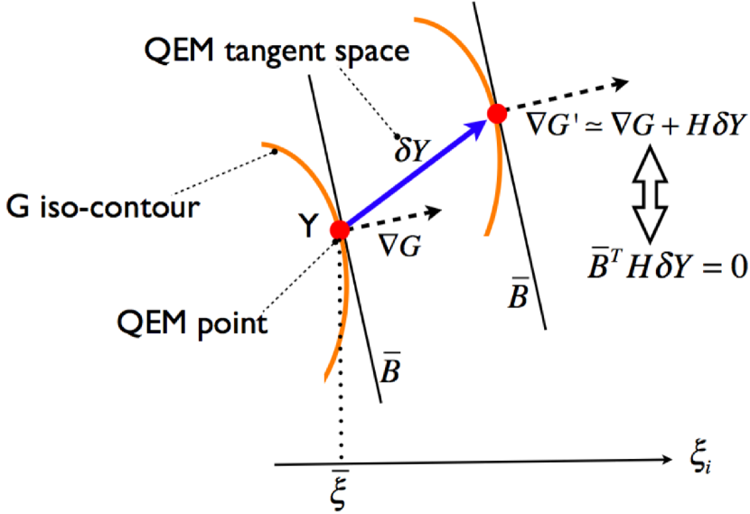
where q𝑞q denotes the QEM dimension, while the r×n𝑟𝑛r\times n matrix D𝐷D imposes the conservation of the number of moles (χi,i=1,,rsubscript𝜒formulae-sequence𝑖𝑖1𝑟\chi_{i,i=1,...,r}) of r𝑟r chemical elements involved in the reaction. In Fig. 3, the geometry behind the notion of QEM is shown schematically. Let H𝐻H and B¯¯𝐵\bar{B} be the second derivative matrix of the Lyapunov function G𝐺G and the null space of the (q+r)×n𝑞𝑟𝑛(q+r)\times n matrix of contraints in (37):

B¯=ker[B1BqD1Dr],D=[D1Dr].formulae-sequence¯𝐵kernelsubscript𝐵1subscript𝐵𝑞subscript𝐷1subscript𝐷𝑟𝐷delimited-[]subscript𝐷1subscript𝐷𝑟\bar{B}=\ker\left[\begin{array}[]{l}B_{1}\\ \vdots\\ B_{q}\\ D_{1}\\ \vdots\\ D_{r}\\ \end{array}\right],\quad D=\left[\begin{array}[]{l}D_{1}\\ \vdots\\ D_{r}\\ \end{array}\right].

Let the n×(nr)𝑛𝑛𝑟n\times(n-r) matrix D¯¯𝐷\bar{D} be defined as follows:

D¯=[D¯1,,D¯nr]=kerD.¯𝐷subscript¯𝐷1subscript¯𝐷𝑛𝑟kernel𝐷\bar{D}=\left[{\bar{D}_{1},...,\bar{D}_{n-r}}\right]=\ker D.

With the basis vectors {D¯1,,D¯nr}subscript¯𝐷1subscript¯𝐷𝑛𝑟\{\bar{D}_{1},...,\bar{D}_{n-r}\} spanning the null space of D𝐷D (kerDkernel𝐷\ker D), an arbitrary vector δY𝛿𝑌\delta Y along the tangent space of a QEM can be written in terms of the vector δ=[δ1,,δnr]T𝛿superscriptsubscript𝛿1subscript𝛿𝑛𝑟𝑇\delta=\left[{\delta_{1},...,\delta_{n-r}}\right]^{T} as:

D¯δ=δY=D¯[δ1δnr].¯𝐷𝛿𝛿𝑌¯𝐷delimited-[]subscript𝛿1subscript𝛿𝑛𝑟\bar{D}\delta=\delta Y=\bar{D}\left[\begin{array}[]{l}\delta_{1}\\ \vdots\\ \delta_{n-r}\\ \end{array}\right]. (38)
Refer to caption
Figure 3: (Color online). Pictorial representation of the notion of quasi-equilibrium manifold (QEM) (37), H𝐻H and B¯¯𝐵\bar{B} being the second derivative matrix of the Lyapunov function G𝐺G and the null space of the full set of constraints in (37), respectively.

The geometry behind the optimization problem (37) imposes the orthogonality condition B¯THD¯δ=0superscript¯𝐵𝑇𝐻¯𝐷𝛿0\bar{B}^{T}H\bar{D}\delta=0 (see also Fig. 3), and the tangent space to a QEM is spanned by:

TQEM=D¯ker(B¯THD¯).subscript𝑇𝑄𝐸𝑀¯𝐷kernelsuperscript¯𝐵𝑇𝐻¯𝐷T_{QEM}=\bar{D}\ker(\bar{B}^{T}H\bar{D}).

Recalling the definition of the matrix A𝐴A in (8), a possible initialization of A𝐴A (with 1:Y=A1ξ+l1\mathcal{F}^{1}:\quad Y=A^{1}\xi+l^{1} describing locally a QEM) takes the form:

A1=TQEM(BTQEM)1,superscript𝐴1subscript𝑇𝑄𝐸𝑀superscript𝐵subscript𝑇𝑄𝐸𝑀1A^{1}=T_{QEM}\left({BT_{QEM}}\right)^{-1}, (39)

whereas 1(ξ¯)=Y1superscript1¯𝜉superscript𝑌1\mathcal{F}^{1}\left(\bar{\xi}\right)=Y^{1} can be found by solving the optimization problem (37) using for example tools suggested in [41] and [8]. Finally, possible choices for the matrix B𝐵B are discussed in [7, 8] (spectral quasi equilibrium parameterization) and [27, 2] (constrained equilibrium parameterization) while exact formulae for computing matrices H𝐻H and J𝐽J can be found in [5, 11].

Moreover, Eq. (30) and the dynamical system (31) require the initial condition A~1=A~(to=0)superscript~𝐴1~𝐴subscript𝑡𝑜0\tilde{A}^{1}=\tilde{A}(t_{o}=0). A possible option is the following: Since fast motions are necessarily transversal to the slow subspace (22), a reasonable choice for the (nqr)×n𝑛𝑞𝑟𝑛(n-q-r)\times n matrix B~~𝐵\tilde{B} reads:

B~=(ker[A1ssAqssD1Dr])T.~𝐵superscriptkernelsubscriptsuperscript𝐴𝑠𝑠1subscriptsuperscript𝐴𝑠𝑠𝑞subscript𝐷1subscript𝐷𝑟𝑇\tilde{B}=\left(\ker\left[\begin{array}[]{l}A^{ss}_{1}\\ \vdots\\ A^{ss}_{q}\\ D_{1}\\ \vdots\\ D_{r}\\ \end{array}\right]\right)^{T}. (40)

As a first guess (k=1𝑘1k=1), let the mapping (25) describe the orthogonal subspace to the SIM (22). More specifically, let the former space be spanned by the columns of the n×(nqr)𝑛𝑛𝑞𝑟n\times(n-q-r) matrix

T=D¯ker[(Ass)TD¯],superscript𝑇bottom¯𝐷kernelsuperscriptsuperscript𝐴𝑠𝑠𝑇¯𝐷T^{\bot}=\bar{D}\ker\left[(A^{ss})^{T}\bar{D}\right], (41)

similarly to (39), initial condition for (30) and (31) takes the explicit form

A~1=T(B~T)1.superscript~𝐴1superscript𝑇bottomsuperscript~𝐵superscript𝑇bottom1\tilde{A}^{1}=T^{\bot}\left(\tilde{B}T^{\bot}\right)^{-1}. (42)

We notice that owing to the relations BA1=I𝐵superscript𝐴1𝐼BA^{1}=I and B~A~1=I~𝐵superscript~𝐴1𝐼\tilde{B}\tilde{A}^{1}=I, as an alternative to (39) and (42), A𝐴A and A~~𝐴\tilde{A} can be initialized by computing the Moore-Penrose pseudoinverse matrices of B𝐵B and B~~𝐵\tilde{B}, respectively.

3.5 Stability and adaptive construction of slow invariant manifolds

Stability of the governing equations of the linearized RRM (21) can be exploited for adaptive construction of SIM. In the first place, Eqs. (21) can be solved with q=1𝑞1q=1: If convergence is experienced, we assume that a 1D reduced model of the system (1) can be constructed in a vicinity of the macrostate ξ¯¯𝜉\bar{\xi}. In other words, a minimal description (2) of the detailed system (1) can be accomplished by means of one degree of freedom. On the contrary, with no convergence, the manifold dimension is updated to q=2𝑞2q=2 and the procedure repeated. Upon convergence with some q=q¯𝑞¯𝑞q=\bar{q}, we may infer that a minimal description of the detailed dynamics requires q¯¯𝑞\bar{q} degrees of freedom. In this sense, the suggested method enables an adaptive construction of SIM (i.e. varying dimension in the phase-space without any a priori assumptions on the value of q𝑞q). The above idea relies upon the assumption that RRM is stable provided the existence of SIM of a certain dimension q𝑞q [13, 12]. More details on the stability of the RRM can be found in [5], where a comparative study between a method for the direct solution of the film equation (5) and RRM is performed.

4 Benchmark
Refer to caption
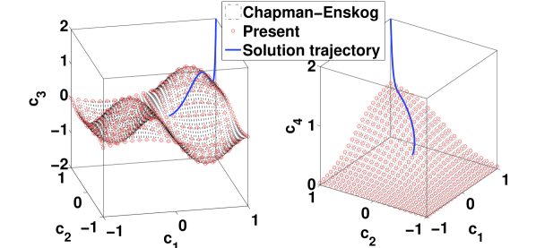
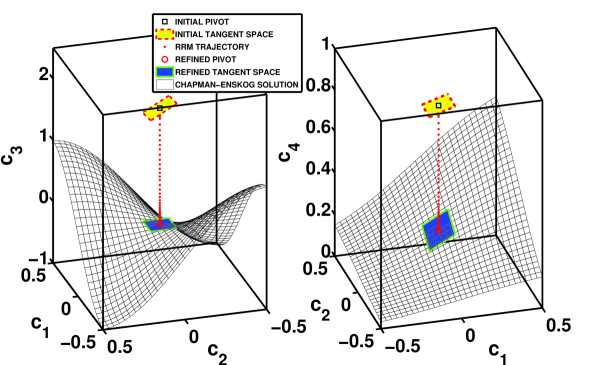
Figure 4: (Color online). Slow invariant manifold with respect to the dynamical system (43) with (49), ω=3𝜔3\omega=3 and ϵ=0.025italic-ϵ0.025\epsilon=0.025. Starting from the initial conditions (50), the governing equations of the linearized RRM (21) with n=4𝑛4n=4, q=2𝑞2q=2 and τ=3×10¹⁰𝜏3superscript1010\tau=3\times 10^{-10} are solved by means of the stiff numerical scheme ode15s readily available in Matlab® [42]. Here, the steady state is reached after an integration time Tf=1subscript𝑇𝑓1T_{f}=1. At steady state, the solution trajectory (dots) finally lands on the SIM.

For the sake of simplicity, we consider here a four-dimensional model where the dynamics of two fast variables (c3subscript𝑐3c_{3} and c4subscript𝑐4c_{4}) is slaved to the motion of the slow variables c1subscript𝑐1c_{1} and c2subscript𝑐2c_{2} [44]. Let the functions f1subscript𝑓1f_{1}, f2subscript𝑓2f_{2}, θ1subscript𝜃1\theta_{1} and θ2subscript𝜃2\theta_{2} depend on c1subscript𝑐1c_{1} and c2subscript𝑐2c_{2} only. In the following, we focus on the ODE system:

dcdt=[f1(c1,c2)f2(c1,c2)1ϵ[c3θ1(c1,c2)]+f1c1θ1(c1,c2)+f2c2θ1(c1,c2)1ϵ[c4θ2(c1,c2)]+f1c1θ2(c1,c2)+f2c2θ2(c1,c2)],𝑑𝑐𝑑𝑡delimited-[]subscript𝑓1subscript𝑐1subscript𝑐2missing-subexpressionmissing-subexpressionmissing-subexpressionmissing-subexpressionmissing-subexpressionmissing-subexpressionmissing-subexpressionmissing-subexpressionmissing-subexpressionmissing-subexpressionmissing-subexpressionmissing-subexpressionmissing-subexpressionmissing-subexpressionmissing-subexpressionmissing-subexpressionmissing-subexpressionmissing-subexpressionmissing-subexpressionsubscript𝑓2subscript𝑐1subscript𝑐2missing-subexpressionmissing-subexpressionmissing-subexpressionmissing-subexpressionmissing-subexpressionmissing-subexpressionmissing-subexpressionmissing-subexpressionmissing-subexpressionmissing-subexpressionmissing-subexpressionmissing-subexpressionmissing-subexpressionmissing-subexpressionmissing-subexpressionmissing-subexpressionmissing-subexpressionmissing-subexpressionmissing-subexpression1italic-ϵdelimited-[]subscript𝑐3subscript𝜃1subscript𝑐1subscript𝑐2subscript𝑓1subscriptsubscript𝑐1subscript𝜃1subscript𝑐1subscript𝑐2subscript𝑓2subscriptsubscript𝑐2subscript𝜃1subscript𝑐1subscript𝑐2missing-subexpressionmissing-subexpressionmissing-subexpressionmissing-subexpressionmissing-subexpressionmissing-subexpressionmissing-subexpressionmissing-subexpressionmissing-subexpressionmissing-subexpressionmissing-subexpressionmissing-subexpressionmissing-subexpressionmissing-subexpressionmissing-subexpressionmissing-subexpressionmissing-subexpressionmissing-subexpressionmissing-subexpression1italic-ϵdelimited-[]subscript𝑐4subscript𝜃2subscript𝑐1subscript𝑐2subscript𝑓1subscriptsubscript𝑐1subscript𝜃2subscript𝑐1subscript𝑐2subscript𝑓2subscriptsubscript𝑐2subscript𝜃2subscript𝑐1subscript𝑐2missing-subexpressionmissing-subexpressionmissing-subexpressionmissing-subexpressionmissing-subexpressionmissing-subexpressionmissing-subexpressionmissing-subexpressionmissing-subexpressionmissing-subexpressionmissing-subexpressionmissing-subexpressionmissing-subexpressionmissing-subexpressionmissing-subexpressionmissing-subexpressionmissing-subexpressionmissing-subexpressionmissing-subexpression\frac{{dc}}{{dt}}=\left[{\begin{array}[]{*{20}c}{f_{1}\left(c_{1},c_{2}\right)}\\ {f_{2}\left(c_{1},c_{2}\right)}\\ {-\frac{1}{\epsilon}\left[c_{3}-\theta_{1}\left(c_{1},c_{2}\right)\right]+f_{1}\partial_{c_{1}}\theta_{1}\left(c_{1},c_{2}\right)+f_{2}\partial_{c_{2}}\theta_{1}\left(c_{1},c_{2}\right)}\\ {-\frac{1}{\epsilon}\left[c_{4}-\theta_{2}\left(c_{1},c_{2}\right)\right]+f_{1}\partial_{c_{1}}\theta_{2}\left(c_{1},c_{2}\right)+f_{2}\partial_{c_{2}}\theta_{2}\left(c_{1},c_{2}\right)}\\ \end{array}}\right], (43)
Refer to caption
Figure 5: (Color online). An array of initial states has been refined by means of the linearized RRM. Stationary states of the (21) are reported (circles). For a comparison, the exact Chapman-Enskog solution and a detailed solution trajectory of the system (43) are also shown. Here we use ω=3𝜔3\omega=3, τ=3×10¹⁰𝜏3superscript1010\tau=3\times 10^{-10}, while integration of (21) is performed for an integration time Tf=1subscript𝑇𝑓1T_{f}=1 at any point. The computational time required to refine the entire array, composed by (21×21)2121(21\times 21) points, was 2.52.52.5 minutes using a Matlab code on a single processor with 1.73 GHz.

where ϵitalic-ϵ\epsilon and isubscript𝑖\partial_{i} denote a fixed small quantity and partial derivative with respect to variable i𝑖i, respectively. Assuming that the dynamics of c3subscript𝑐3c_{3} and c4subscript𝑐4c_{4} is slaved to the slow variables,

c3=c3(c1,c2),c4=c4(c1,c2).formulae-sequencesubscript𝑐3subscript𝑐3subscript𝑐1subscript𝑐2subscript𝑐4subscript𝑐4subscript𝑐1subscript𝑐2c_{3}=c_{3}\left(c_{1},c_{2}\right),\;c_{4}=c_{4}\left(c_{1},c_{2}\right). (44)

and, according to the chain rule, time derivatives of (44) take the explicit form:

dc3dt=c1c3dc1dt+c2c3dc2dt=c1c3f1+c2c3f2,dc4dt=c1c4dc1dt+c2c4dc2dt=c1c4f1+c2c4f2.𝑑subscript𝑐3𝑑𝑡subscriptsubscript𝑐1subscript𝑐3𝑑subscript𝑐1𝑑𝑡subscriptsubscript𝑐2subscript𝑐3𝑑subscript𝑐2𝑑𝑡subscriptsubscript𝑐1subscript𝑐3subscript𝑓1subscriptsubscript𝑐2subscript𝑐3subscript𝑓2missing-subexpressionmissing-subexpressionmissing-subexpressionmissing-subexpressionmissing-subexpressionmissing-subexpressionmissing-subexpressionmissing-subexpressionmissing-subexpressionmissing-subexpressionmissing-subexpressionmissing-subexpressionmissing-subexpressionmissing-subexpressionmissing-subexpressionmissing-subexpressionmissing-subexpressionmissing-subexpressionmissing-subexpression𝑑subscript𝑐4𝑑𝑡subscriptsubscript𝑐1subscript𝑐4𝑑subscript𝑐1𝑑𝑡subscriptsubscript𝑐2subscript𝑐4𝑑subscript𝑐2𝑑𝑡subscriptsubscript𝑐1subscript𝑐4subscript𝑓1subscriptsubscript𝑐2subscript𝑐4subscript𝑓2missing-subexpressionmissing-subexpressionmissing-subexpressionmissing-subexpressionmissing-subexpressionmissing-subexpressionmissing-subexpressionmissing-subexpressionmissing-subexpressionmissing-subexpressionmissing-subexpressionmissing-subexpressionmissing-subexpressionmissing-subexpressionmissing-subexpressionmissing-subexpressionmissing-subexpressionmissing-subexpressionmissing-subexpression{\begin{array}[]{*{20}c}\frac{dc_{3}}{dt}=\partial_{c_{1}}c_{3}\frac{dc_{1}}{dt}+\partial_{c_{2}}c_{3}\frac{dc_{2}}{dt}=\partial_{c_{1}}c_{3}f_{1}+\partial_{c_{2}}c_{3}f_{2},\\ \frac{dc_{4}}{dt}=\partial_{c_{1}}c_{4}\frac{dc_{1}}{dt}+\partial_{c_{2}}c_{4}\frac{dc_{2}}{dt}=\partial_{c_{1}}c_{4}f_{1}+\partial_{c_{2}}c_{4}f_{2}.\\ \end{array}} (45)
Refer to caption
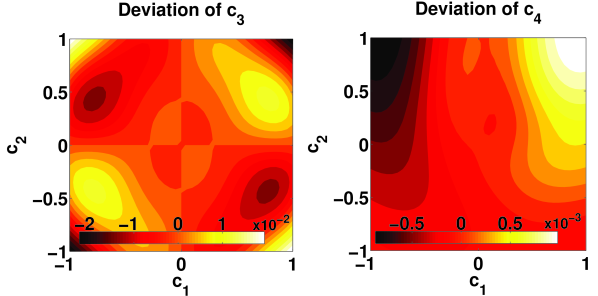
Figure 6: (Color online). Difference between the SIM constructed by the linearized RRM method as reported in Fig. 5 and the Chapman-Enskog solution (c3=θ1subscript𝑐3subscript𝜃1c_{3}=\theta_{1}, c4=θ2subscript𝑐4subscript𝜃2c_{4}=\theta_{2}).

Upon substituting equations (45) in (43), one obtains the following invariance conditions with respect to (43) (see also section 2 and Eq. (4)):

c1c3f1+c2c3f2=1ϵ[c3θ1(c1,c2)]+f1c1θ1(c1,c2)+f2c2θ1(c1,c2),c1c4f1+c2c4f2=1ϵ[c4θ2(c1,c2)]+f1c1θ2(c1,c2)+f2c2θ2(c1,c2).subscriptsubscript𝑐1subscript𝑐3subscript𝑓1subscriptsubscript𝑐2subscript𝑐3subscript𝑓21italic-ϵdelimited-[]subscript𝑐3subscript𝜃1subscript𝑐1subscript𝑐2subscript𝑓1subscriptsubscript𝑐1subscript𝜃1subscript𝑐1subscript𝑐2subscript𝑓2subscriptsubscript𝑐2subscript𝜃1subscript𝑐1subscript𝑐2missing-subexpressionmissing-subexpressionmissing-subexpressionmissing-subexpressionmissing-subexpressionmissing-subexpressionmissing-subexpressionmissing-subexpressionmissing-subexpressionmissing-subexpressionmissing-subexpressionmissing-subexpressionmissing-subexpressionmissing-subexpressionmissing-subexpressionmissing-subexpressionmissing-subexpressionmissing-subexpressionmissing-subexpressionsubscriptsubscript𝑐1subscript𝑐4subscript𝑓1subscriptsubscript𝑐2subscript𝑐4subscript𝑓21italic-ϵdelimited-[]subscript𝑐4subscript𝜃2subscript𝑐1subscript𝑐2subscript𝑓1subscriptsubscript𝑐1subscript𝜃2subscript𝑐1subscript𝑐2subscript𝑓2subscriptsubscript𝑐2subscript𝜃2subscript𝑐1subscript𝑐2missing-subexpressionmissing-subexpressionmissing-subexpressionmissing-subexpressionmissing-subexpressionmissing-subexpressionmissing-subexpressionmissing-subexpressionmissing-subexpressionmissing-subexpressionmissing-subexpressionmissing-subexpressionmissing-subexpressionmissing-subexpressionmissing-subexpressionmissing-subexpressionmissing-subexpressionmissing-subexpressionmissing-subexpression{\begin{array}[]{*{20}c}{\partial_{c_{1}}c_{3}f_{1}+\partial_{c_{2}}c_{3}f_{2}=-\frac{1}{\epsilon}\left[c_{3}-\theta_{1}\left(c_{1},c_{2}\right)\right]+f_{1}\partial_{c_{1}}\theta_{1}\left(c_{1},c_{2}\right)+f_{2}\partial_{c_{2}}\theta_{1}\left(c_{1},c_{2}\right),}\\ {\partial_{c_{1}}c_{4}f_{1}+\partial_{c_{2}}c_{4}f_{2}=-\frac{1}{\epsilon}\left[c_{4}-\theta_{2}\left(c_{1},c_{2}\right)\right]+f_{1}\partial_{c_{1}}\theta_{2}\left(c_{1},c_{2}\right)+f_{2}\partial_{c_{2}}\theta_{2}\left(c_{1},c_{2}\right).}\\ \end{array}} (46)

A common approach to obtain solutions to the above invariance conditions is the Chapman-Enskog method [4, 45], which is based on the assumption that ϵitalic-ϵ\epsilon is small compared to all other quantities, and it is implemented by series expansions of the (44) in powers of ϵitalic-ϵ\epsilon:

c3(c1,c2)=c3(0)+ϵc3(1)+ϵ2c3(2)+c4(c1,c2)=c4(0)+ϵc4(1)+ϵ2c4(2)+subscript𝑐3subscript𝑐1subscript𝑐2superscriptsubscript𝑐30italic-ϵsuperscriptsubscript𝑐31superscriptitalic-ϵ2superscriptsubscript𝑐32missing-subexpressionmissing-subexpressionmissing-subexpressionmissing-subexpressionmissing-subexpressionmissing-subexpressionmissing-subexpressionmissing-subexpressionmissing-subexpressionmissing-subexpressionmissing-subexpressionmissing-subexpressionmissing-subexpressionmissing-subexpressionmissing-subexpressionmissing-subexpressionmissing-subexpressionmissing-subexpressionmissing-subexpressionsubscript𝑐4subscript𝑐1subscript𝑐2superscriptsubscript𝑐40italic-ϵsuperscriptsubscript𝑐41superscriptitalic-ϵ2superscriptsubscript𝑐42missing-subexpressionmissing-subexpressionmissing-subexpressionmissing-subexpressionmissing-subexpressionmissing-subexpressionmissing-subexpressionmissing-subexpressionmissing-subexpressionmissing-subexpressionmissing-subexpressionmissing-subexpressionmissing-subexpressionmissing-subexpressionmissing-subexpressionmissing-subexpressionmissing-subexpressionmissing-subexpressionmissing-subexpression{\begin{array}[]{*{20}c}c_{3}\left(c_{1},c_{2}\right)=c_{3}^{(0)}+\epsilon c_{3}^{(1)}+\epsilon^{2}c_{3}^{(2)}+...\\ c_{4}\left(c_{1},c_{2}\right)=c_{4}^{(0)}+\epsilon c_{4}^{(1)}+\epsilon^{2}c_{4}^{(2)}+...\\ \end{array}} (47)

Hence, the first equation in (46) reads:

f1c1[c3(0)+ϵc3(1)+ϵ2c3(2)+]+f2c2[c3(0)+ϵc3(1)+ϵ2c3(2)+]=1ϵ[c3(0)+ϵc3(1)+ϵ2c3(2)+θ1]+f1c1θ1+f2c2θ1.subscript𝑓1subscriptsubscript𝑐1delimited-[]superscriptsubscript𝑐30italic-ϵsuperscriptsubscript𝑐31superscriptitalic-ϵ2superscriptsubscript𝑐32subscript𝑓2subscriptsubscript𝑐2delimited-[]superscriptsubscript𝑐30italic-ϵsuperscriptsubscript𝑐31superscriptitalic-ϵ2superscriptsubscript𝑐321italic-ϵdelimited-[]superscriptsubscript𝑐30italic-ϵsuperscriptsubscript𝑐31superscriptitalic-ϵ2superscriptsubscript𝑐32subscript𝜃1subscript𝑓1subscriptsubscript𝑐1subscript𝜃1subscript𝑓2subscriptsubscript𝑐2subscript𝜃1\begin{split}f_{1}\partial_{c_{1}}\left[c_{3}^{(0)}+\epsilon c_{3}^{(1)}+\epsilon^{2}c_{3}^{(2)}+...\right]+f_{2}\partial_{c_{2}}\left[c_{3}^{(0)}+\epsilon c_{3}^{(1)}+\epsilon^{2}c_{3}^{(2)}+...\right]=\\ -\frac{1}{\epsilon}\left[c_{3}^{(0)}+\epsilon c_{3}^{(1)}+\epsilon^{2}c_{3}^{(2)}+...-\theta_{1}\right]+f_{1}\partial_{c_{1}}\theta_{1}+f_{2}\partial_{c_{2}}\theta_{1}.\end{split}

After collecting terms with the same power of ϵitalic-ϵ\epsilon, we obtain:

c3(0)=θ1(c1,c2),c3(i)=0,i>0,formulae-sequencesuperscriptsubscript𝑐30subscript𝜃1subscript𝑐1subscript𝑐2formulae-sequencesuperscriptsubscript𝑐3𝑖0for-all𝑖0c_{3}^{(0)}=\theta_{1}\left(c_{1},c_{2}\right),\;c_{3}^{(i)}=0,\;\forall i>0, (48)

namely c3=θ1(c1,c2)subscript𝑐3subscript𝜃1subscript𝑐1subscript𝑐2c_{3}=\theta_{1}\left(c_{1},c_{2}\right), and similarly c4=θ2(c1,c2)subscript𝑐4subscript𝜃2subscript𝑐1subscript𝑐2c_{4}=\theta_{2}\left(c_{1},c_{2}\right).

For illustration purposes, we choose:

θ1(c1,c2)=sin(ωc1)sin(ωc2),θ2(c1,c2)=[(1+eωc1)(1+eωc2)]1,f1=c1,f2=2c2.formulae-sequencesubscript𝜃1subscript𝑐1subscript𝑐2sin𝜔subscript𝑐1sin𝜔subscript𝑐2subscript𝜃2subscript𝑐1subscript𝑐2superscriptdelimited-[]1superscript𝑒𝜔subscript𝑐11superscript𝑒𝜔subscript𝑐21missing-subexpressionmissing-subexpressionmissing-subexpressionmissing-subexpressionmissing-subexpressionmissing-subexpressionmissing-subexpressionmissing-subexpressionmissing-subexpressionmissing-subexpressionmissing-subexpressionmissing-subexpressionmissing-subexpressionmissing-subexpressionmissing-subexpressionmissing-subexpressionmissing-subexpressionmissing-subexpressionmissing-subexpressionformulae-sequencesubscript𝑓1subscript𝑐1subscript𝑓22subscript𝑐2missing-subexpressionmissing-subexpressionmissing-subexpressionmissing-subexpressionmissing-subexpressionmissing-subexpressionmissing-subexpressionmissing-subexpressionmissing-subexpressionmissing-subexpressionmissing-subexpressionmissing-subexpressionmissing-subexpressionmissing-subexpressionmissing-subexpressionmissing-subexpressionmissing-subexpressionmissing-subexpressionmissing-subexpression{\begin{array}[]{*{20}l}\theta_{1}\left(c_{1},c_{2}\right)={\rm sin}\left(\omega c_{1}\right){\rm sin}\left(\omega c_{2}\right),\;\theta_{2}\left(c_{1},c_{2}\right)=\left[\left(1+e^{-\omega c_{1}}\right)\left(1+e^{-\omega c_{2}}\right)\right]^{-1},\\ f_{1}=-c_{1},\;f_{2}=-2c_{2}.\end{array}} (49)

In Fig. 4, the Chapman-Enskog solution to (46) is plotted to illustrate the relaxation of system (21), starting from the following initial pivot and tangent space:

Y¯1=[0,0,1.9,0.85]T,A1=[10010.2761.4050.2250.0282].formulae-sequencesuperscript¯𝑌1superscript001.90.85𝑇superscript𝐴1delimited-[]10missing-subexpressionmissing-subexpressionmissing-subexpressionmissing-subexpressionmissing-subexpressionmissing-subexpressionmissing-subexpressionmissing-subexpressionmissing-subexpressionmissing-subexpressionmissing-subexpressionmissing-subexpressionmissing-subexpressionmissing-subexpressionmissing-subexpressionmissing-subexpressionmissing-subexpressionmissing-subexpression01missing-subexpressionmissing-subexpressionmissing-subexpressionmissing-subexpressionmissing-subexpressionmissing-subexpressionmissing-subexpressionmissing-subexpressionmissing-subexpressionmissing-subexpressionmissing-subexpressionmissing-subexpressionmissing-subexpressionmissing-subexpressionmissing-subexpressionmissing-subexpressionmissing-subexpressionmissing-subexpression0.2761.405missing-subexpressionmissing-subexpressionmissing-subexpressionmissing-subexpressionmissing-subexpressionmissing-subexpressionmissing-subexpressionmissing-subexpressionmissing-subexpressionmissing-subexpressionmissing-subexpressionmissing-subexpressionmissing-subexpressionmissing-subexpressionmissing-subexpressionmissing-subexpressionmissing-subexpressionmissing-subexpression0.2250.0282missing-subexpressionmissing-subexpressionmissing-subexpressionmissing-subexpressionmissing-subexpressionmissing-subexpressionmissing-subexpressionmissing-subexpressionmissing-subexpressionmissing-subexpressionmissing-subexpressionmissing-subexpressionmissing-subexpressionmissing-subexpressionmissing-subexpressionmissing-subexpressionmissing-subexpressionmissing-subexpression\bar{Y}^{1}=\left[{0,0,1.9,0.85}\right]^{T},\;\;A^{1}=\left[{\begin{array}[]{*{20}c}1&0\\ 0&1\\ {-0.276}&{-1.405}\\ {0.225}&{0.0282}\\ \end{array}}\right]. (50)

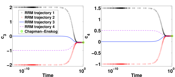
Finally, the SIM parameterization is chosen as follows: ξ1=c1subscript𝜉1subscript𝑐1\xi_{1}=c_{1}, ξ2=c2subscript𝜉2subscript𝑐2\xi_{2}=c_{2}. We stress that, in the computations, the steady state (Y¯sssuperscript¯𝑌𝑠𝑠\bar{Y}^{ss}, Asssuperscript𝐴𝑠𝑠A^{ss}) does not depend on the initial choice of Y¯1superscript¯𝑌1\bar{Y}^{1} and A1superscript𝐴1A^{1} (see Fig. 7). The latter observation is consistent with the idea behind the RRM [12], which can be elucidated by saying that states on the SIM represent stable steady states of the dynamical system (21).
Refer to caption
Figure 7: (Color online). On the basis of the system (43) with (49), ω=3𝜔3\omega=3 and ϵ=0.025italic-ϵ0.025\epsilon=0.025, we solve (21) by means of the numerical scheme ode15s [42] starting from several initial conditions Y¯1superscript¯𝑌1\bar{Y}^{1} and A1superscript𝐴1A^{1}, with fixed parameters ξ1=c1=0.3subscript𝜉1subscript𝑐10.3\xi_{1}=c_{1}=0.3 and ξ2=c2=0.2subscript𝜉2subscript𝑐20.2\xi_{2}=c_{2}=-0.2. Time evolution of c3subscript𝑐3c_{3} and c4subscript𝑐4c_{4}, as dictated by (21), is reported. For an integration time Tf>1subscript𝑇𝑓1T_{f}>1, the steady state is reached such that c3ss=0.4422superscriptsubscript𝑐3𝑠𝑠0.4422c_{3}^{ss}=-0.4422, c4ss=0.2520superscriptsubscript𝑐4𝑠𝑠0.2520c_{4}^{ss}=0.2520 for any initial conditions. At steady state, small deviations from the Chapman-Enskog solution (star) are observed (smaller than 0.01%).

The reduced system (2) for the above example (43) rules the evolution of the slow variables:

dc1dt=f1=c1dc2dt=f2=2c2𝑑subscript𝑐1𝑑𝑡subscript𝑓1subscript𝑐1missing-subexpressionmissing-subexpressionmissing-subexpressionmissing-subexpressionmissing-subexpressionmissing-subexpressionmissing-subexpressionmissing-subexpressionmissing-subexpressionmissing-subexpressionmissing-subexpressionmissing-subexpressionmissing-subexpressionmissing-subexpressionmissing-subexpressionmissing-subexpressionmissing-subexpressionmissing-subexpressionmissing-subexpression𝑑subscript𝑐2𝑑𝑡subscript𝑓22subscript𝑐2missing-subexpressionmissing-subexpressionmissing-subexpressionmissing-subexpressionmissing-subexpressionmissing-subexpressionmissing-subexpressionmissing-subexpressionmissing-subexpressionmissing-subexpressionmissing-subexpressionmissing-subexpressionmissing-subexpressionmissing-subexpressionmissing-subexpressionmissing-subexpressionmissing-subexpressionmissing-subexpressionmissing-subexpression{\begin{array}[]{*{20}l}\frac{dc_{1}}{dt}=f_{1}=-c_{1}\\ \frac{dc_{2}}{dt}=f_{2}=-2c_{2}\end{array}} (51)

whereas fast variables can be reconstructed by means of the mappings c3=c3(c1,c2)subscript𝑐3subscript𝑐3subscript𝑐1subscript𝑐2c_{3}=c_{3}(c_{1},c_{2}), c4=c4(c1,c2)subscript𝑐4subscript𝑐4subscript𝑐1subscript𝑐2c_{4}=c_{4}(c_{1},c_{2}) (Fig. 5).

In this respect, in Fig. 8, a solution trajectory of (43) is compared to the trajectory of (51), where the reconstruction of c3subscript𝑐3c_{3} and c4subscript𝑐4c_{4} is performed using both the exact Chapman-Enskog solution (c3=θ1subscript𝑐3subscript𝜃1c_{3}=\theta_{1}, c4=θ2subscript𝑐4subscript𝜃2c_{4}=\theta_{2}) and a linear look up table based on the nodes refined by the linearized RRM (see also Figs. 5 and 6).
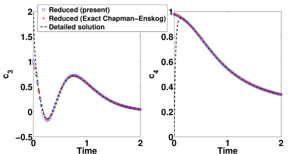
Refer to caption
Figure 8: (Color online). Comparison between the detailed solution of the system (43) from the state c1=1.5subscript𝑐11.5c_{1}=1.5, c2=1.5subscript𝑐21.5c_{2}=1.5, c3=2subscript𝑐32c_{3}=2, c4=0subscript𝑐40c_{4}=0 (out of SIM) and the reduced solution of the system (51) from the state c1=1.5subscript𝑐11.5c_{1}=1.5, c2=1.5subscript𝑐21.5c_{2}=1.5. The numerical stiff solver ode15s [42] is used with ω=3𝜔3\omega=3, ϵ=0.025italic-ϵ0.025\epsilon=0.025 and τ=3×10¹⁰𝜏3superscript1010\tau=3\times 10^{-10}.
τ𝜏\tau c1sssuperscriptsubscript𝑐1𝑠𝑠c_{1}^{ss} c2sssuperscriptsubscript𝑐2𝑠𝑠c_{2}^{ss} c3sssuperscriptsubscript𝑐3𝑠𝑠c_{3}^{ss} c4sssuperscriptsubscript𝑐4𝑠𝑠c_{4}^{ss}
1×10131superscript10131\times 10^{-13} 0.60.6-0.6 0.850.85-0.85 0.5512716057066630.551271605706663{0.551271605706663} 0.0100236946455480.010023694645548{0.010023694645548}
1×10121superscript10121\times 10^{-12} 0.60.6-0.6 0.850.85-0.85 0.5512716020387360.551271602038736{0.551271602038736} 0.0100236957834660.010023695783466{0.010023695783466}
1×10111superscript10111\times 10^{-11} 0.60.6-0.6 0.850.85-0.85 0.5512715981941130.551271598194113{0.551271598194113} 0.0100236970183950.010023697018395{0.010023697018395}
1×10101superscript10101\times 10^{-10} 0.60.6-0.6 0.850.85-0.85 0.5512715967624280.551271596762428{0.551271596762428} 0.0100236974701800.010023697470180{0.010023697470180}
1×1091superscript1091\times 10^{-9} 0.60.6-0.6 0.850.85-0.85 0.5512716056202280.551271605620228{0.551271605620228} 0.0100236946728330.010023694672833{0.010023694672833}
1×1081superscript1081\times 10^{-8} - - - -
Table 1: The steady state (c1sssuperscriptsubscript𝑐1𝑠𝑠c_{1}^{ss}, c2sssuperscriptsubscript𝑐2𝑠𝑠c_{2}^{ss}, c3sssuperscriptsubscript𝑐3𝑠𝑠c_{3}^{ss}, c4sssuperscriptsubscript𝑐4𝑠𝑠c_{4}^{ss}) of (21) is computed for several choices of the parameter τ𝜏\tau starting from the state c1=0.6subscript𝑐10.6c_{1}=-0.6, c2=0.85subscript𝑐20.85c_{2}=-0.85, c3=1subscript𝑐31c_{3}=-1, c4=0.5subscript𝑐40.5c_{4}=0.5, with ω=3𝜔3\omega=3 and ϵ=0.025italic-ϵ0.025\epsilon=0.025. No convergence is observed for τ1×10⁸𝜏1superscript108\tau\geq 1\times 10^{-8}.

In Table 1, we report a sensitivity analysis with respect to the parameter τ𝜏\tau. We notice that an estimate of the time scales of a dynamical system can be obtained by a spectral decomposition of the Jacobi matrix. For the case in Fig. 5, at equilibrium (c1=c2=c3=0subscript𝑐1subscript𝑐2subscript𝑐30c_{1}=c_{2}=c_{3}=0, c4=0.25subscript𝑐40.25c_{4}=0.25):

τ1=τ2=1|λ1|=1|λ2|=3.72×10¹⁰,τ3=1|λ3|=7.45×10⁹,τ4=1|λ4|=1.49×10⁸,formulae-sequencesubscript𝜏1subscript𝜏21subscript𝜆11subscript𝜆23.72superscript1010subscript𝜏31subscript𝜆37.45superscript109subscript𝜏41subscript𝜆41.49superscript108\begin{split}\tau_{1}=\tau_{2}=\frac{1}{\left|\lambda_{1}\right|}=\frac{1}{\left|\lambda_{2}\right|}=3.72\times 10^{-10},\;\tau_{3}=\frac{1}{\left|\lambda_{3}\right|}=7.45\times 10^{-9},\\ \tau_{4}=\frac{1}{\left|\lambda_{4}\right|}=1.49\times 10^{-8},\end{split}

where λisubscript𝜆𝑖\lambda_{i} denotes the i𝑖i-th eigenvalue. Hence, in the above computations we use τ=3×10¹⁰𝜏3superscript1010\tau=3\times 10^{-10}. However, the latter parameters was varied within a wide range of values and no significant effect was noticed on both the stability of (21) and the value of its steady state.

In addition, we test the equations (31) for computing the mapping (25) describing the local fast subspace. To this end, we make use of (40) and (42) (with D=D¯=1𝐷¯𝐷1D=\bar{D}=1, r=0𝑟0r=0).

At steady state of (31), we observe (at any node of the grid in Fig. 5) that the columns of the matrix A~~𝐴\tilde{A} span the subspace defined by the vectors:

[0,0,1,0],[0,0,0,1],00100001\left[{0,0,1,0}\right],\quad\left[{0,0,0,1}\right],

in accordance with the assumption that c3subscript𝑐3c_{3} and c4subscript𝑐4c_{4} are the fast variables.

Refer to caption
Figure 9: (Color online). Model for the hydrogen-air combustion [36] in a closed system under fixed enthalpy (500kJ/kg500𝑘𝐽𝑘𝑔500kJ/kg) and pressure (1bar1𝑏𝑎𝑟1bar). Initialization is accomplished using (37) and (39), where the matrix B𝐵B is chosen according to the spectral quasi equilibrium parameterization [7]. Here, an arbitrary state on a two dimensional QEM is driven on a two dimensional SIM by solving the governing equations of the linearized RRM (21), with n=9𝑛9n=9, q=2𝑞2q=2, r=3𝑟3r=3, τ=1×10⁹𝜏1superscript109\tau=1\times 10^{-9} using the stiff numerical scheme ode15s readily available in Matlab® [42].

Finally, the governing equations of the linearized RRM (21) were applied to a more complicated case of the detailed reaction mechanism for combustion of hydrogen in air [36]. Here, Eq. (21) were tested for computing states of the SIM with dimensions up to q=5𝑞5q=5. In Fig. 9, we report an example with q=2𝑞2q=2.

Moreover, we observed that any steady state of (31) corresponds to a matrix A~~𝐴\tilde{A} whose columns are linear combinations of the fast eigenvectors of Jsssuperscript𝐽𝑠𝑠J^{ss} (i.e., eigenvectors corresponding to the nqr𝑛𝑞𝑟n-q-r largest eigenvalues in absolute value).

5 Conclusions and outlook

Based on the rationale behind the film equation (5) and the Relaxation Redistribution Method (RRM), a set of ordinary differential equations (ODEs) is obtained with the aim of mimicking the only fast relaxation of a multiscale dynamical system towards a slow invariant manifold (SIM). This approach is characterized by a straightforward implementation consisting in solving the ODEs by state of the art stiff numerical schemes, and it proves useful for constructing accurate approximations of SIM in any dimensions.

It is worth stressing that, like RRM, convergence of equations (21) towards a steady state might be used for a fully adaptive construction of heterogeneous (i.e. varying dimension in different regions of the phase-space) slow invariant manifolds.

This work sheds light on the connection between the RRM method and the solution of both the invariance and film equations as postulated in [5, 13, 12] (see discussion at the end of section 3.1).

In addition, the novel algorithm (31) for approximating the fast subspace is suggested, and a possible initialization procedure for both (21) and (31) is proposed.

The methods are tested in the case of detailed combustion of hydrogen and air, as well as in a benchmark problem of a model with exact Chapman-Enskong solution of the invariance equation.

We stress that, although the presented methodology has been tested in the case of dissipative systems with a unique steady state (see Section 4), in this paper we show that the governing equations (21) and (31) of the linearized RRM are based on the general notions of film equation (5) and SIM (local) parameterization. Therefore, investigations on the performance of the presented method in more general systems with multiple steady states and chaotic behavior (see, e.g., [17, 23]) are planned for future publications. However, in the latter case, new initialization procedures are needed since the method discussed in Section 3.4 is suitable for dissipative systems equipped with thermodynamic Lyapunov function.

Finally, it is worth noticing that the proposed approach represents only one possible implementation of the RRM method ([5, 13, 12]). More accurate descriptions of the SIM (to be addressed in future publications) can be obtained as well, abandoning the present linear expressions (8) and (12) in favor of higher order approximations.

6 Acknowledgments

I. Kevrekidis and B. Sonday are gratefully acknowledged for suggesting the model (43) with the functions (49). The Author wishes to thank S. Pope and I. Karlin for inspiring discussions. Acknowledgments go to C. Frouzakis and all Referees for their valuable help in improving the quality of the manuscript.

References

  • [1] A. Adrover, F. Creta, M. Giona, and M. Valorani. Stretching-based diagnostics and reduction of chemical kinetic models with diffusion. J. Comput. Phys, 225:1442–1471, 2007.
  • [2] P. Bishnu, D. Hamiroune, and M. Metghalchi. Development of constrained equilibrium codes and their applications in nonequilibrium thermodynamics. ASME, 123:214–220, 2001.
  • [3] V. Bykov and U. Maas. The extension of the ILDM concept to reaction-diffusion manifolds. Combust. Theory Modelling, 11:839–862, 2007.
  • [4] S. Chapman and T. G. Cowling. The Mathematical Theory of Non-uniform Gases. Cambridge Mathematical Library, 1999.
  • [5] E. Chiavazzo. Invariant Manifolds and Lattice Boltzmann Method for Combustion. PhD thesis, Swiss Federal Institute of Technology, ETH-Zurich, 2009.
  • [6] E. Chiavazzo, P. Asinari, and F. Visconti. Fast computation of multi-scale combustion systems. Phil. Trans. Royal Society A, 369:2396–2404, 2011.
  • [7] E. Chiavazzo, A. N. Gorban, and I. V. Karlin. Comparison of invariant manifolds for model reduction in chemical kinetics. Comm. in Comput. Physics, 2:964–992, 2007.
  • [8] E. Chiavazzo and I. V. Karlin. Quasi-equilibrium grid algorithm: Geometric construction for model reduction. J. Comput. Phys., 227:5535–5560, 2008.
  • [9] E. Chiavazzo, I. V. Karlin, and A. N. Gorban. The role of thermodynamics in model reduction when using invariant grids. Comm. in Comput. Physics, 8:701–734, 2010.
  • [10] E. Chiavazzo, I. V. Karlin, A. N. Gorban, and K. Boulouchos. Combustion simulation via lattice boltzmann and reduced chemical kinetics. JSTAT, P01013, 2009.
  • [11] E. Chiavazzo, I. V. Karlin, A. N. Gorban, and K. Boulouchos. Coupling of the model reduction technique with the lattice boltzmann method for combustion simulations. Combust. Flame, 157:1833–1849, 2010.
  • [12] E. Chiavazzo and I.V. Karlin. Adaptive simplification of complex multiscale systems. Phys. Rev. E, 83:036706, 2011.
  • [13] E. Chiavazzo and I.V. Karlin. Adaptive Simplification of Complex Systems: A Review of the Relaxation-Redistribution Approach. In A. Gorban and D. Roose, editors, Coping with Complexity: Model Reduction and Data Analysis, pages 231–240. Springer, 2011.
  • [14] R. Courant, K. O. Friedrichs, and H. Lewy. On the partial difference equations of mathematical physics. IBM J., 11:215–234, 1967.
  • [15] D. Endy and R. Brent. Modelling cellular behaviour. Nature, 409:391–395, 2001.
  • [16] N. Fenichel. Geometric singular perturbation theory for ordinary differential equations. J. Diff. Equ., 31:53–98, 1979.
  • [17] I.T. Georgiou, J.C. Martin, and A.K. Bajaj. Dynamics of nonlinear structures with multiple equilibria: A singular perturbation-invariant manifold approach. Z. Angew. Math. Phys., 50:892–924, 1999.
  • [18] A. N. Gorban and I. V. Karlin. Invariant Manifolds for Physical and Chemical Kinetics. Springer, Berlin, 2005.
  • [19] A. N. Gorban, I. V. Karlin, and A. Y. Zinovyev. Invariant grids for reaction kinetics. Physica A, 333:106–154, 2004.
  • [20] A. N. Gorban, N. Kazantzis, I. G. Kevrekidis, H. C. Öttinger, and C. Theodoropoulos, editors. Model Reduction and Coarse-graining Approaches for Multiscale Phenomena, Berlin, 2006. Springer.
  • [21] D. Goussis and U. Maas. Model reduction for combustion chemistry. In T. Echekki and E. Mastorakos, editors, Turbulent Combustion Modeling, pages 193–220. Springer Science, 2011.
  • [22] D.A. Goussis and M. Valorani. An efficient iterative algorithm for the approximation of the fast and slow dynamics of stiff systems. J. Comput. Phys., 214:316–346, 2006.
  • [23] G. Haller and T. Sapsis. Localized instability and attraction along invariant manifolds. SIAM J. App. Dyn. Syst., 9:611–633, 2010.
  • [24] D. Hamiroune, P. Bishnu, M. Metghalchi, and J. C. Keck. Rate-controlled constrained-equilibrium method using constraint potentials. Combust. Theory Model., 2:81–94, 1998.
  • [25] N. Jamshidi and B. Ø Palsson. Formulating genome-scale kinetic models in the post-genome era. Molecular Systems Biology, 4:171, 2008.
  • [26] N. Kazantis, C. Kravaris, and L. Syrou. A new model reduction method for nonlinear dynamical systems. Nonlinear Dynamics, 59:183–194, 2010.
  • [27] J. C. Keck and D. Gillespie. Rate-controlled partial-equilibrium method for treating reacting gas-mixtures. Combust. Flame, 17:237–241, 1971.
  • [28] P. D. Kourdis, D. A. Goussis, and R. Steuer. Physical Understanding via Reduction of Complex Multiscale Models: Glycolysis in Saccharomyces cerevisie. BioInformatics and BioEngineering, BIBE 2008. 8th IEEE, 2008.
  • [29] S. H. Lam and D. A. Goussis. Conventional asymptotic and computational singular perturbation for symplified kinetics modelling. Springer, Berlin, 1991.
  • [30] D. Lebiedz. Computing minimal entropy production trajectories: An approach to model reduction in chemical kinetics. J. Chem. Phys., 120:6890–6897, 2004.
  • [31] D. Lebiedz. Entropy-Related Extremum Principles for Model Reduction of Dissipative Dynamical Systems. Entropy, 12:706–719, 2010.
  • [32] D. Lebiedz, J. Kammerer, and U. Brandt-Pollmann. Automatic network coupling analysis for dynamical systems based on detailed kinetic models. Phys. Rev. E, page 041911, 2005.
  • [33] D. Lebiedz, V. Reinhardt, and J. Siehrb. Minimal curvature trajectories: Riemannian geometry concepts for slow manifold computation in chemical kinetics. J. Comput. Phys., 229:6512–6533, 2010.
  • [34] D. Lebiedz, J. Siehr, and J. Unger. A variational principle for computing slow invariant manifolds in dissipative dynamical systems. SIAM J. Sci. Comput., 33:703, 2011.
  • [35] D. Lebiedz, D. Skanda, and M. Fein. Automatic complexity analysis and model reduction of nonlinear biochemical systems. In M. Heiner and A. Uhrmacher, editors, Computational Methods in Systems Biology, pages 123–140. Springer, 2008.
  • [36] J. Li, Z. Zhao, A. Kazakov, and F. L. Dryer. Int. J. Chem. Kinet., 36:566–575, 2004.
  • [37] A. M. Lyapunov. The general problem of the stability of motion. Taylor & Francis, 1992.
  • [38] U. Maas and S. B. Pope. Simplifying chemical kinetics: Intrinsic low-dimensional manifolds in composition space. Combust. Flame, 88:239–264, 1992.
  • [39] J. Nafe and U. Maas. A general algorithm for improving ILDMs. Combust. Theory Modelling, 6:697–709, 2002.
  • [40] Z. Ren, S. B. Pope, A. Vladimirsky, and J. M. Guckenheimer. The invariant constrained equilibrium edge preimage curve method for the dimension reduction of chemical kinetics. J. Chem. Phys., 124:114111, 2006.
  • [41] W. C. Reynolds. The element potential method for chemical equilibrium analysis: Implementation in the interactive program stanjan. Mechanical Engineering Department, Standford University, 1986.
  • [42] L. F. Shampine and M. W. Reichelt. The MATLAB ODE Suite. SIAM Journal on Scientific Computing, 18:1, 1997.
  • [43] G. P. Smith, D. M. Golden, M. Frenklach, N. W. Moriarty, B. Eiteneer, M. Goldenberg, C. T. Bowman, R. K. Hanson, S. Song, W. C. Gardiner, V.V. Lissianski, and Z. Qin. http://www.me.berkeley.edu/gri_mech/. 1999.
  • [44] B. Sonday. The corresponding dynamics of any desired slow manifold. private communication, 2011.
  • [45] H. Struchtrup. Macroscopic Transport Equations for Rarefied Gas Flows. Springer, Berlin, 2005.
  • [46] I. Surovtsova, N. Simus, T. Lorenz, A. König, S. Sahle, and U. Kummer. Accessible methods for the dynamic time-scale decomposition of biochemical systems. BIOINFORMATICS, 25:2816–2823, 2009.
  • [47] M. Valorani, D. A. Goussis, and H. N. Najm. Higher order corrections in the approximation of low-dimensional manifolds and the construction of simplified problems with the csp method. J. Comput. Phys., 209:754–786, 2005.
  • [48] M. Valorani and S. Paolucci. The G-Scheme: A framework for multi-scale adaptive model reduction. J. Comput. Phys., 228:4665–4701, 2009.