Calculation of High Energy Neutrino-Nucleon Cross Sections and Uncertainties Using the MSTW Parton Distribution Functions and Implications for Future Experiments

Abstract

We present a new calculation of the cross sections for charged current (CC) and neutral current (NC) $\nu N$ and $\bar{\nu}N$ interactions in the neutrino energy range $10^{4}<E_{\nu}<10^{12}$ GeV using the most recent MSTW parton distribution functions (PDFs), MSTW 2008. We also present the associated uncertainties propagated from the PDFs, as well as parametrizations of the cross section central values, their uncertainty bounds, and the inelasticity distributions for ease of use in Monte Carlo simulations. For the latter we only provide parametrizations for energies above $10^{7}$ GeV. Finally, we assess the feasibility of future neutrino experiments to constrain the $\nu N$ cross section in the ultra-high energy (UHE) regime using a technique that is independent of the flux spectrum of incident neutrinos. A significant deviation from the predicted Standard Model cross sections could be an indication of new physics, such as extra space-time dimensions, and we present expected constraints on such models as a function of the number of events observed in a future subterranean neutrino detector.

I Introduction

Neutrino experiments are closing in on neutrinos in the ultra-high energy (UHE) regime, where a diffuse neutrino flux, first predicted by Berezinsky and Zatsepin Berezinsky and Zatsepin (1969, 1970), is expected to result from interactions between UHE cosmic rays and cosmic microwave background photons through what is known as the Greisen, Zatsepin and Kuzmin (GZK) process Greisen (1966); Zatsepin and Kuzmin (1966). Neutrinos in this energy regime probe higher center-of-mass (COM) energies than those accessible by human-made accelerators through their interactions in the earth. For example, the COM energy of a $10^{9}$ GeV neutrino incident on a nucleon at rest is 45 TeV. Thus, a measurement of neutrino-nucleon ($\nu N$) cross sections in the UHE regime could be sensitive to either new physics scenarios such as extra space-time dimensions or unexpected behavior of parton distribution functions (PDFs) at Bjorken-$x$ smaller than that accessible by current experiments (from here on, any $\nu$ refers to both neutrino and anti-neutrino unless otherwise stated) Anchordoqui et al. (2006a). However, before the significance of any $\nu N$ cross section measurement can be assessed, the uncertainties on the Standard Model (SM) expectation must be quantified based on the diverse body of current experimental constraints.

The paper is composed of two parts. In Section II, we perform a new calculation of $\nu N$ cross sections and their associated PDF uncertainties for neutrino energies $E_{\nu}>10^{4}$ GeV using the MSTW 2008 PDF set. In Section II.1, we review the expressions for the $\nu N$ cross sections in terms of the quark PDFs. In Section II.2 we present the results of our cross section calculations, associated uncertainties and their energy dependent parametrizations. Next, in Section II.3 we discuss the differential cross sections, and parametrize the inelasticity distributions in an energy dependent way. We also show a few select distributions in $x$. In Section II.4, we calculate the correlations between the uncertainties across energies.

In Section III, we propose to constrain the UHE $\nu N$ cross section in future sub-terranean neutrino experiments using a technique that is independent of the incident flux spectrum of neutrinos and present projected constraints on models with enhanced cross sections due to extra space-time dimensions.

II Neutrino-Nucleon Cross Section

II.1 Methodology

The $\nu N$ cross section for charged current (CC) interactions on an isoscalar target is given by :

$$\sigma_{CC}\left(E_{\nu}\right)=\frac{2G_{F}^{2}M_{N}E_{\nu}}{\pi}\int_{0}^{1}\int_{0}^{1}dy~{}dx\left(\frac{M_{W}^{2}}{Q^{2}+M_{W}^{2}}\right)^{2}\left[q+\left(1-y\right)^{2}\bar{q}\right]$$ (1)

with quark and antiquark densities given by $q=(d+u)/2+s+b$ and $\bar{q}=(\bar{d}+\bar{u})/2+c+t$. In all of the equations in this paper we assume that a quark distribution function is equivalent to the corresponding antiparticle distribution except for $u$ and $d$. In MSTW 2008, $t=0$ and it is not strictly true that $s=\bar{s}$, but these are negligible effects for our calculations. Here, $G_{F}=1.17\times 10^{-5}$ GeV^-2 is the Fermi coupling constant and $M_{N}$ is the nucleon mass for which we use the proton mass, 0.938 GeV. The mass of the $W$ boson $M_{W}=80.398$ GeV, $E_{\nu}$ is the incident neutrino energy, and $x$ and $y$ are the parton momentum fraction (Bjorken-$x$) and the inelasticity, respectively.

Likewise, the neutral current (NC) $\nu N$ cross section is given by:

$$\sigma_{NC}\left(E_{\nu}\right)=\frac{2G_{F}^{2}M_{N}E_{\nu}}{\pi}\int_{0}^{1}\int_{0}^{1}dy~{}dx\left(\frac{M_{Z}^{2}}{Q^{2}+M_{Z}^{2}}\right)^{2}\left[q^{0}+\left(1-y\right)^{2}\bar{q^{0}}\right]$$ (2)

where $M_{Z}$ is the $Z$ mass. Then

$$q^{0} =\frac{u+d}{2}\left(L_{u}^{2}+L_{d}^{2}\right)+\frac{\bar{u}+\bar{d}}{2}\left(R_{u}^{2}+R_{d}^{2}\right)+$$ (3)

$$\left(s+b\right)\left(L_{d}^{2}+R_{d}^{2}\right)+\left(c+t\right)\left(L_{u}^{2}+R_{u}^{2}\right)$$ (4)

and

$$\bar{q^{0}}= \frac{u+d}{2}\left(R_{u}^{2}+R_{d}^{2}\right)+\frac{\bar{u}+\bar{d}}{2}\left(L_{u}^{2}+L_{d}^{2}\right)$$ (5)

$$+\left(s+b\right)\left(L_{d}^{2}+R_{d}^{2}\right)+\left(c+t\right)\left(L_{u}^{2}+R_{u}^{2}\right)$$ (6)

with $L_{u}=1-4/3\cdot x_{W}$, $L_{d}=-1+2/3\cdot x_{W}$, $R_{u}=-4/3\cdot x_{W}$ and $R_{d}=2/3\cdot x_{W}$ where $x_{W}=\sin^{2}{\theta_{W}}=0.226$. For the $\bar{\nu}$N cross sections, the above equations are the same with each quark distribution function replaced with the corresponding antiparticle distribution and vice versa, so that $q\leftrightarrow\bar{q}$, $q^{0}\leftrightarrow\bar{q^{0}}$.

We use the parton distribution functions calculated by A.D. Martin et al. known as “MSTW 2008” Martin et al. (2009). These PDFs are the latest update to a series that began with the MRS PDFs twenty years ago, which were the first global next-to-leading-order (NLO) PDF analysis. The MSTW 2008 set incorporates improvements in the precision and kinematic range of recent measurements as well as improved theoretical developments which make the global analysis more reliable. The publication of the MSTW 2008 set was particularly timely in view of the start of data taking at the Large Hadron Collider (LHC).

II.2 Cross Sections

Figs. 1 and 2 shows the results of our $\nu N$ and $\bar{\nu}N$ cross section calculations compared to the previous calculations by Gandhi et al. (GQRS) Gandhi et al. (1998). These results are summarized numerically in Tables 1 and 2. With regard to uncertainties, the latter paper only states that they find the uncertainties in the $\nu N$ cross sections to be at most a factor of $2^{\pm 1}$. Recently Cooper-Sarkar and Sarkar (CSS) Cooper-Sarkar and Sarkar (2008) also published CC $\nu N$ cross sections for energies in the range $100<s<10^{12}$ GeV² where $\sqrt{s}$ is the COM energy of the interaction. There has also been a recent investigation into the dependence on the number of active heavy quarks in  Jeong and Reno (2010). We find good agreement with the central values of both the GQRS and CSS calculations within our uncertainties. We note that the explicit evolution of the MSTW 2008 PDFs only takes place down to the lowest value of the grid points, i.e. $x=10^{-6}$. Below this the values for the central set and each eigenvector for the error sets are extrapolated linearly in $\ln(1/x)$. Within the region of the grids the accuracy of the NLO and NNLO evolution has been checked to small fractions of a percent, see Section 3 of Martin et al. (2009).

Figure 1: Calculated $\nu N$ CC and NC cross sections. In this plot we compare this work (CTW), with the shaded bands representing the associated uncertainties due to PDFs, to those in Gandhi et al. (GQRS). Thin black lines bound the NC uncertainties so that they remain visible where they overlap with the CC bounds.

Figure 2: Calculated $\bar{\nu}N$ CC and NC cross sections. In this plot we compare this work (CTW), with the shaded bands representing the associated uncertainties due to PDFs, to those in GQRS.

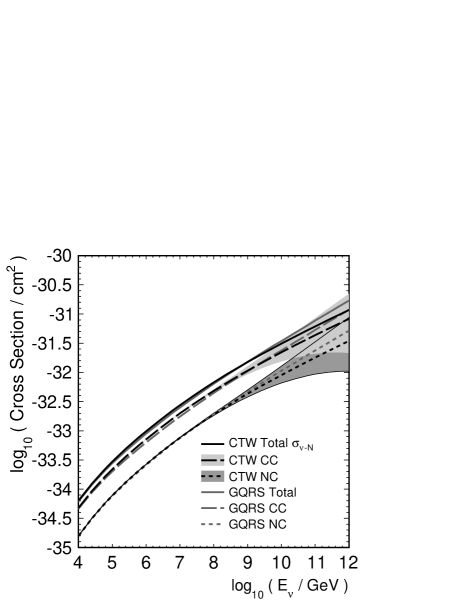
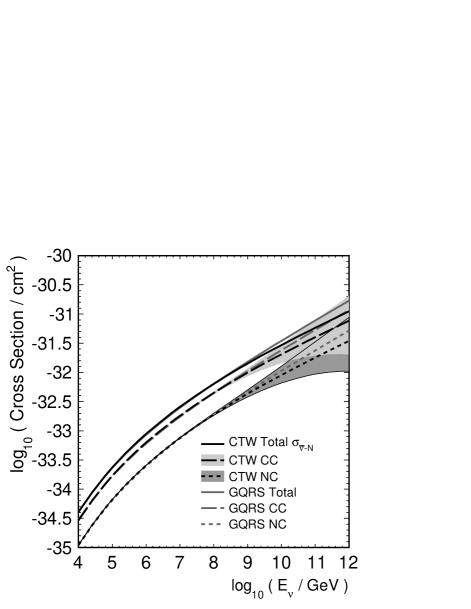
Fig. 3 compares the uncertainties on the cross section calculations for the range of energies being considered. The uncertainties on our calculations are dramatically different from those reported by CSS for $E_{\nu}\gtrsim 10^{8}$ GeV. The difference is due to a different parametrization of the gluon parton distribution $g\left(x\right)$. The CSS fit to the HERA data allows a very good fit with the gluon distribution having an $x$ dependence of the form $g\left(x\right)~{}\propto~{}x^{\delta}$. However, MSTW 2008 finds that a sum of two terms with different powers $xg\left(x\right)~{}\propto~{}A_{1}x^{\delta_{1}}+A_{2}x^{\delta_{2}}$ gives a better fit to the global data set. This is partially due to the global fit requiring a slightly larger value of the strong coupling $\alpha_{S}$ and consequently less gluon to drive small-$x$ structure function evolution. It is also found that Tevatron jet data prefer a larger high-$x$ gluon distribution, hence allowing a smaller gluon distribution at small-$x$ from the momentum sum rule. (It is shown in Martin et al. (2010) that fitting the newer combined HERA data in Aaron et al. (2010) results in no very significant change to the MSTW PDFs.)

Figure 3: Uncertainties on the calculated cross sections due to PDFs. We compare this work (CTW) to CSS.

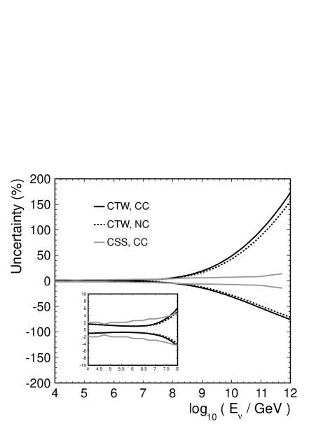
As well as producing the best fit, the greater flexibility brought about by including two terms in the parametrization results in more rapid expansion of the allowed range in $g\left(x\right)$ at low-$x$ beyond the reach of current experiments, as illustrated in Fig. 16 of Martin et al. (2009). With the parametrization used by CSS, the uncertainty can only grow as a function of $\ln\left(1/x\right)$ in this region as discussed in Section 6.5 of Martin et al. (2009). We notice that the point at which our uncertainty starts to exceed that of CSS to a significant extent is indeed when the constraint due to HERA data is starting to disappear, i.e. when the dominant $x$ values contributing to the cross section are $x=10^{-5}$ or lower. At very high neutrino energy when the $x$ values probed are typically well below $x=10^{-5}$ our uncertainty on the cross section becomes very large. Hence, we conclude that a good measurement of the cross section within this range will provide the first direct constraint on the extremely small-$x$ PDFs, and can give us the first true indication of their central value as well as reducing the uncertainty significantly.

At the lower end of the uncertainty bands the cross sections do contain contributions from PDFs that have become negative. It is difficult to know whether this is really a problem. At low orders in $\alpha_{S}$ and leading twist perturbation theory this could lead to negative cross sections. However, we have the possibility of both large $\ln(1/x)$ perturbative corrections and higher-twist nonlinear effects in this regime which could alter this conclusion. Hence, our uncertainty at the very highest energies can be thought of as acknowledging the possibility of theoretical corrections in this regime.

The recent comparative study of high energy neutrino cross sections in Goncalves and Hepp (2010) illustrates the variation between models at very high energies due to theoretical assumptions. (Note the variation at lower energies between models in Figs. 1 and 2 of this paper is likely due to the omission of terms required at higher $x$ Thorne (2005)).

Table 1: Cross Sections for $\nu$N.

$E_{\nu}$ (GeV)	$\sigma_{\rm{CC}}$ (cm-2)	$\sigma_{\rm{NC}}$ (cm-2)	$\sigma_{\rm{tot}}$ (cm-2)
1 $\times 10^{4}$	0.48$\times 10^{-34}$	0.16$\times 10^{-34}$	0.63$\times 10^{-34}$
2.5 $\times 10^{4}$	0.93$\times 10^{-34}$	0.32$\times 10^{-34}$	0.12$\times 10^{-33}$
6 $\times 10^{4}$	0.16$\times 10^{-33}$	0.57$\times 10^{-34}$	0.22$\times 10^{-33}$
1 $\times 10^{5}$	0.22$\times 10^{-33}$	0.78$\times 10^{-34}$	0.3$\times 10^{-33}$
2.5 $\times 10^{5}$	0.36$\times 10^{-33}$	0.13$\times 10^{-33}$	0.49$\times 10^{-33}$
6 $\times 10^{5}$	0.56$\times 10^{-33}$	0.21$\times 10^{-33}$	0.77$\times 10^{-33}$
1 $\times 10^{6}$	0.72$\times 10^{-33}$	0.27$\times 10^{-33}$	0.98$\times 10^{-33}$
2.5 $\times 10^{6}$	0.11$\times 10^{-32}$	0.41$\times 10^{-33}$	0.15$\times 10^{-32}$
6 $\times 10^{6}$	0.16$\times 10^{-32}$	0.61$\times 10^{-33}$	0.22$\times 10^{-32}$
1 $\times 10^{7}$	0.2$\times 10^{-32}$	0.76$\times 10^{-33}$	0.27$\times 10^{-32}$
2.5 $\times 10^{7}$	0.29$\times 10^{-32}$	0.11$\times 10^{-32}$	0.4$\times 10^{-32}$
6 $\times 10^{7}$	0.4$\times 10^{-32}$	0.16$\times 10^{-32}$	0.56$\times 10^{-32}$
1 $\times 10^{8}$	0.48$\times 10^{-32}$	0.19$\times 10^{-32}$	0.67$\times 10^{-32}$
2.5 $\times 10^{8}$	0.67$\times 10^{-32}$	0.27$\times 10^{-32}$	0.94$\times 10^{-32}$
6 $\times 10^{8}$	0.91$\times 10^{-32}$	0.36$\times 10^{-32}$	0.13$\times 10^{-31}$
1 $\times 10^{9}$	0.11$\times 10^{-31}$	0.43$\times 10^{-32}$	0.15$\times 10^{-31}$
2.5 $\times 10^{9}$	0.14$\times 10^{-31}$	0.58$\times 10^{-32}$	0.2$\times 10^{-31}$
6 $\times 10^{9}$	0.19$\times 10^{-31}$	0.77$\times 10^{-32}$	0.27$\times 10^{-31}$
1 $\times 10^{10}$	0.22$\times 10^{-31}$	0.9$\times 10^{-32}$	0.31$\times 10^{-31}$
2.5 $\times 10^{10}$	0.29$\times 10^{-31}$	0.12$\times 10^{-31}$	0.41$\times 10^{-31}$
6 $\times 10^{10}$	0.37$\times 10^{-31}$	0.15$\times 10^{-31}$	0.53$\times 10^{-31}$
1 $\times 10^{11}$	0.43$\times 10^{-31}$	0.18$\times 10^{-31}$	0.61$\times 10^{-31}$
2.5 $\times 10^{11}$	0.56$\times 10^{-31}$	0.23$\times 10^{-31}$	0.8$\times 10^{-31}$
6 $\times 10^{11}$	0.72$\times 10^{-31}$	0.3$\times 10^{-31}$	0.1$\times 10^{-30}$
1 $\times 10^{12}$	0.83$\times 10^{-31}$	0.35$\times 10^{-31}$	0.12$\times 10^{-30}$

Table 2: Cross Sections for $\bar{\nu}$N.

$E_{\bar{\nu}}$ (GeV)	$\sigma_{\rm{CC}}$ (cm-2)	$\sigma_{\rm{NC}}$ (cm-2)	$\sigma_{\rm{tot}}$ (cm-2)
1 $\times 10^{4}$	0.29$\times 10^{-34}$	0.11$\times 10^{-34}$	0.4$\times 10^{-34}$
2.5 $\times 10^{4}$	0.63$\times 10^{-34}$	0.24$\times 10^{-34}$	0.87$\times 10^{-34}$
6 $\times 10^{4}$	0.12$\times 10^{-33}$	0.47$\times 10^{-34}$	0.17$\times 10^{-33}$
1 $\times 10^{5}$	0.17$\times 10^{-33}$	0.67$\times 10^{-34}$	0.24$\times 10^{-33}$
2.5 $\times 10^{5}$	0.3$\times 10^{-33}$	0.12$\times 10^{-33}$	0.42$\times 10^{-33}$
6 $\times 10^{5}$	0.49$\times 10^{-33}$	0.2$\times 10^{-33}$	0.68$\times 10^{-33}$
1 $\times 10^{6}$	0.63$\times 10^{-33}$	0.26$\times 10^{-33}$	0.89$\times 10^{-33}$
2.5 $\times 10^{6}$	0.98$\times 10^{-33}$	0.4$\times 10^{-33}$	0.14$\times 10^{-32}$
6 $\times 10^{6}$	0.15$\times 10^{-32}$	0.6$\times 10^{-33}$	0.21$\times 10^{-32}$
1 $\times 10^{7}$	0.18$\times 10^{-32}$	0.76$\times 10^{-33}$	0.26$\times 10^{-32}$
2.5 $\times 10^{7}$	0.26$\times 10^{-32}$	0.11$\times 10^{-32}$	0.37$\times 10^{-32}$
6 $\times 10^{7}$	0.37$\times 10^{-32}$	0.16$\times 10^{-32}$	0.52$\times 10^{-32}$
1 $\times 10^{8}$	0.45$\times 10^{-32}$	0.19$\times 10^{-32}$	0.64$\times 10^{-32}$
2.5 $\times 10^{8}$	0.62$\times 10^{-32}$	0.27$\times 10^{-32}$	0.88$\times 10^{-32}$
6 $\times 10^{8}$	0.84$\times 10^{-32}$	0.36$\times 10^{-32}$	0.12$\times 10^{-31}$
1 $\times 10^{9}$	0.99$\times 10^{-32}$	0.43$\times 10^{-32}$	0.14$\times 10^{-31}$
2.5 $\times 10^{9}$	0.13$\times 10^{-31}$	0.58$\times 10^{-32}$	0.19$\times 10^{-31}$
6 $\times 10^{9}$	0.17$\times 10^{-31}$	0.77$\times 10^{-32}$	0.25$\times 10^{-31}$
1 $\times 10^{10}$	0.2$\times 10^{-31}$	0.9$\times 10^{-32}$	0.29$\times 10^{-31}$
2.5 $\times 10^{10}$	0.27$\times 10^{-31}$	0.12$\times 10^{-31}$	0.39$\times 10^{-31}$
6 $\times 10^{10}$	0.35$\times 10^{-31}$	0.15$\times 10^{-31}$	0.5$\times 10^{-31}$
1 $\times 10^{11}$	0.4$\times 10^{-31}$	0.18$\times 10^{-31}$	0.58$\times 10^{-31}$
2.5 $\times 10^{11}$	0.52$\times 10^{-31}$	0.23$\times 10^{-31}$	0.75$\times 10^{-31}$
6 $\times 10^{11}$	0.66$\times 10^{-31}$	0.3$\times 10^{-31}$	0.96$\times 10^{-31}$
1 $\times 10^{12}$	0.77$\times 10^{-31}$	0.35$\times 10^{-31}$	0.11$\times 10^{-30}$

II.2.1 Parametrizations

For ease of use in Monte Carlo simulations, we have parametrized the cross sections in the energy range $4<\varepsilon<12$, where $\varepsilon\equiv\log_{10}(E_{\nu}/\rm{GeV})$, with an expression of the following form:

$$\begin{array}[]{lcc}\log_{10}\left[\sigma\left(\varepsilon\right)/\rm{cm}^{2}\right]&=&C_{1}+C_{2}\cdot\ln\left(\varepsilon-C_{0}\right)\\ &&+C_{3}\cdot\ln^{2}\left(\varepsilon-C_{0}\right)\\ &&+C_{4}/\ln\left(\varepsilon-C_{0}\right).\\ \end{array}$$ (7)

Table 3: Coefficients for parametrizing the cross sections according to Equation 7.

		$C_{0}$	$C_{1}$	$C_{2}$	$C_{3}$	$C_{4}$
$\nu$	NC	-1.826	-17.31	-6.448	1.431	-18.61
$\nu$	CC			-6.406		-17.91
$\bar{\nu}$	NC	-1.033	-15.95	-7.296	1.569	-18.30
$\bar{\nu}$	CC			-7.247		-17.72

Table 4: Coefficients for parametrizing the uncertainty bounds on the cross sections according to Equation 7.

		$C_{0}$	$C_{1}$	$C_{2}$	$C_{3}$	$C_{4}$
upper
$\nu$	NC	-1.456	32.23	-32.32	5.881	-49.41
$\nu$	CC		33.47	-33.02	6.026
$\bar{\nu}$	NC	-2.945	143.2	-76.70	11.75	-142.8
$\bar{\nu}$	CC		144.5	-77.44	11.90
lower
$\nu$	NC	-15.35	16.16	37.71	-8.801	-253.1
$\nu$	CC		13.86	39.84	-9.205
$\bar{\nu}$	NC	-13.08	15.17	31.19	-7.757	-216.1
$\bar{\nu}$	CC		12.48	33.52	-8.191

Table 3 shows the values of the constants for each of $\nu N$ and $\bar{\nu}N$ interactions, CC and NC. The parametrized cross sections are within approximately 1% (2%) of the calculated cross sections in the stated energy range for $\nu N$ ($\bar{\nu}N$). In Table 4 we show the same constants for parametrizing the upper and lower bounds on the cross sections due to the uncertainties derived in this paper. For the upper bounds, the parametrizations are good to approximately 5% (10%) for describing our $\nu N$ ($\bar{\nu}N$) calculations. For the lower bounds, the parametrizations are at most approximately 8% from our $\nu N$ ($\bar{\nu}N$) calculations until $10^{11.5}<E_{\nu}<10^{12}$ GeV where they deviate by nearly 20%.

Note that the highest power of $\log_{10}E_{\nu}$ required to describe the cross section is quadratic, the same as the quadratic dependence of the Froissart bound Froissart (1961) on hadron-hadron cross sections. This shows that although in principle the PDFs and cross sections grow quicker than any power of $\log_{10}E_{\nu}$ as $E_{\nu}\to\infty$ without some non-linear evolution effects slowing the evolution at very small $x$, in practice this has not clearly manifested itself in the region of energy we consider. The desire to have a parametrization for structure functions manifestly consistent with the Froissart bound at all energies has led to the results in Berger et al. (2008); Block et al. (2010), which gives rather lower predictions than our central values. However, even the upper band of our uncertainty is not generating behaviour obviously stronger than $(\log_{10}E_{\nu})^{2}$ for $E_{\nu}\leq 10^{12}$ GeV.

Finally, the fraction of NC events is parametrized by:

$$\frac{\sigma_{\rm{NC}}}{\sigma_{\rm{NC}}+\sigma_{\rm{CC}}}=D_{1}+D_{2}\cdot\ln\left(\varepsilon-D_{0}\right)$$ (8)

with $D_{0}=1.76$, $D_{1}=0.252162$ and $D_{2}=0.0256$.

II.3 Differential Cross Sections

II.3.1 Inelasticity

For ease of use in Monte Carlo programs, we describe here a procedure for choosing inelasticities that follow the proper energy-dependent distributions for energies in the range $10^{7}\leq E_{\nu}\leq 10^{12}$ GeV. We use the Inverse Transform Method described in Amsler et al. (2008), which requires finding a function that describes $d\sigma/dy$ which has an integral that is invertible.

Due to the steepness of the differential cross section at low values of $y$, we divide up the parametrization into two regions in $y$:

$$\frac{d\sigma}{dy}=\left\{\begin{array}[]{l l}Y(C_{0},C_{1},C_{2})&\quad\mbox{$0<y<10^{-3}$}\\ Y^{\prime}(C_{0}^{\prime},C_{1}^{\prime})&\quad\mbox{$10^{-3}<y<1$}\\ \end{array}\right.$$ (9)

with $Y$ and $Y^{\prime}$ taking the following form:

$$Y\left(C_{0},C_{1},C_{2}\right)=\frac{C_{0}}{(y-C_{1})^{1/C_{2}}}.$$ (10)

$$Y^{\prime}\left(C_{0}^{\prime},C_{1}^{\prime}\right)=\frac{C^{\prime}_{0}}{y-C_{1}^{\prime}}.$$ (11)

For the low $y$ region, the normalized integral of the distribution at $y_{0}$ is:

$$I\left(y_{0}\right)=\frac{\int_{y_{\rm{min}}}^{y_{0}}{Y\left(C_{0},C_{1},C_{2}\right)dy}}{\int_{y_{\rm{min}}}^{y_{\rm{max}}}{Y\left(C_{0},C_{1},C_{2}\right)dy}}=\frac{(y_{0}-C_{1})^{(-1/C_{2}+1)}-(y_{\rm min}-C_{1})^{(-1/C_{2}+1)}}{(y_{\rm max}-C_{1})^{(-1/C_{2}+1)}-(y_{\rm min}-C_{1})^{(-1/C_{2}+1)}}.$$ (12)

For the high $y$ region, it is:

$$I\left(y_{0}\right)=\frac{\int_{y_{\rm{min}}}^{y_{0}}{Y^{\prime}\left(C_{0}^{\prime},C_{1}^{\prime}\right)dy}}{\int_{y_{\rm{min}}}^{y_{\rm{max}}}{Y^{\prime}\left(C_{0}^{\prime},C_{1}^{\prime}\right)dy}}=\left[\frac{\ln{\left(\frac{y_{0}-C_{1}^{\prime}}{y_{\rm{min}}-C_{1}^{\prime}}\right)}}{\ln{\left(\frac{y_{\rm{max}}-C_{1}^{\prime}}{y_{\rm{min}}-C_{1}^{\prime}}\right)}}\right].$$ (13)

Notice that Equations 12 and 13 no longer contain the normalization factors $C_{0}$ and $C_{0}^{\prime}$. For the low-$y$ region, $y_{\rm{min}}=0$ and $y_{\rm{max}}=10^{-3}$, while for the high-$y$ region, $y_{\rm{min}}=10^{-3}$ and $y_{\rm{max}}=1$.

Since Equations 12 and 13 each represent a cumulative distribution function that is invertible, we can use the Inverse Transform Method to select values of $y_{0}$ that follow the distributions in Equation 10 and 11 in each region. By setting $I(y_{0})$ of Equations 12 and 13 to a random number R between 0 and 1, we can then solve for our choice of $y_{0}$ and obtain for the low $y$ region:

$$y_{0}=C_{1}+\left[R(y_{\rm max}-C_{1})^{(-1/C_{2}+1)}+(1-R)(y_{\rm min}-C_{1})^{(-1/C_{2}+1)}\right]^{C_{2}/(C_{2}-1)}$$ (14)

and for the high $y$ region:

$$y_{0}=\frac{(y_{\rm{max}}-C_{1}^{\prime})^{R}}{(y_{\rm{min}}-C_{1}^{\prime})^{R-1}}+C_{1}^{\prime}$$ (15)

The parameter $C_{1}$ itself depends on $\varepsilon$, and for both regions of $y$, the energy dependent parameter takes the form:

$$C_{1}=A_{0}-A_{1}\exp{\left[-\left(\varepsilon-A_{2}\right)/A_{3}\right]}.$$ (16)

In Equation 16, all parameters are primed when describing the high-$y$ region. The numerical values of the parameters in Equation 16, summarized in Table 5, were obtained from fits of the parametrizations to the theoretical calculations.

In the low region, the parameter $C_{2}$ is also energy dependent:

$$C_{2}=B_{0}+B_{1}\cdot\varepsilon$$ (17)

where $B_{0}=2.55$ and $B_{1}=-0.0949$ for all interaction types.

The fraction of the cross section occupying the low-$y$ region is given by:

$$f(\varepsilon)=F_{0}\cdot\sin{[F_{1}\cdot(\varepsilon-F_{2})]}$$ (18)

with $F_{0}=0.128$, $F_{1}=-0.197$ and $F_{2}=21.8$ for all interaction types.

To summarize, for an interaction of a given type ($\nu N$ or $\bar{\nu}N$, CC or NC) at an energy $\varepsilon$, one can find an inelasticity $y_{0}$ chosen from the appropriate distribution through the following steps:

• Choose a random number $R_{1}$ between 0 and 1 and if $R_{1}<f(\epsilon)$ (see Equation 18), then the event lies in the low-$y$ region. Otherwise, it is in the high-$y$ region.

• Obtain the value of $C_{1}^{\prime}$, or $C_{1}$ and $C_{2}$, depending on the $y$ region and the event type, using Equations 16, Equation 17 and Table 5.

• Choose a new random number $R_{2}$ and insert $R=R_{2}$ along with the parameters obtained in the previous step into Equation 14 or Equation 15 to obtain $y_{0}$.

Figs. 4 and 5 show the calculated $y$ distributions in each region compared with the event distributions generated from this procedure for $\nu N$, CC events at $\varepsilon=12$.

Figure 4: Comparison of the $\nu N$ CC inelasticity distributions from our theoretical calculation (black line) and the distribution obtained from the parametrization procedure described in Section II.3.1 (gray histogram).

Figure 5: Same as Fig. 4, but for low-$y$ region.

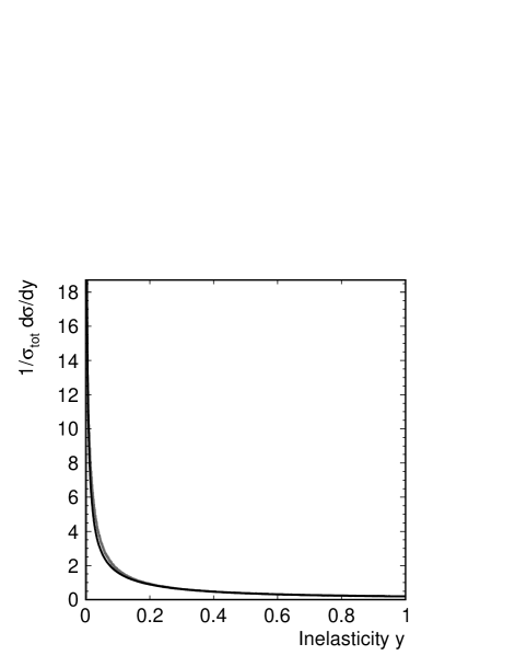
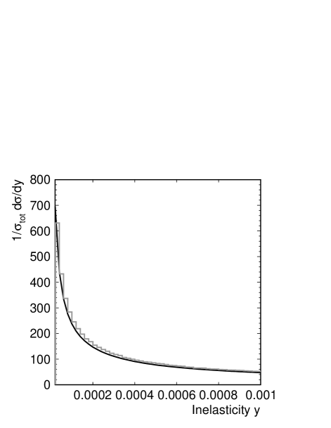
For all event types and energies in the range $7\leq\varepsilon\leq 12$, this procedure will give $y$ distributions whose mean value differs from the theoretical calculation by at most 3.7% in the energy range $E_{\nu}=10^{7}-10^{12}$ GeV. Recall that the inelasticity is the fraction of neutrino energy carried away by the hadronic shower and therefore these uncertainties on the mean hadronic energy imply less than 1% uncertainties on the mean energy of the final state lepton. The RMS of the distributions are 0.05-0.07 in the same energy range and the difference in RMS values between the model and the calculation is no more than 2.6% for all interaction types except the $\bar{\nu}N$ CC events, whose uncertainties on the RMS values do not exceed 8.3%. In Bulmahn and Reno (2010), the authors give a parametrization of the inelasticity distributions in the neutrino energy range 50 GeV$<E_{\nu}<10^{12}$ GeV which are within 15% agreement with calculations using the CTEQ6 parton distribution functions.

Sample code for generating energy dependent inelasticity distributions for all interaction types according to the prescription laid out in this paper can be found at:
http://www.physics.ohio-state.edu/$\mathtt{\sim}$connolly/crosssections/y.html.

Table 5: Coefficients that go into calculating $C_{1}$ and $C_{1}^{\prime}$ in Equation 16 for parametrizing the inelasticity distributions.

low $y$
	$A_{0}$	$A_{1}$	$A_{2}$	$A_{3}$
	0.0	0.0941	4.72	0.456
high $y$
	$A^{\prime}_{0}$	$A^{\prime}_{1}$	$A^{\prime}_{2}$	$A^{\prime}_{3}$
$\bar{\nu}N$ CC	-0.0026	0.085	4.1	1.7
$\nu N$ CC	-0.008	0.26	3.0
$\bar{\nu}N$ NC	-0.005	0.23	3.0	1.7
$\nu N$ NC

II.3.2 Bjorken-$x$

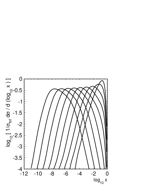
The fraction of momentum carried by a parton within a nucleon is called the Bjorken-$x$. UHE neutrino cross sections include contributions from PDFs in the region of $x$ that is lower than the region above $10^{-4}-10^{-5}$ accessible in the perturbative regime by HERA experiments Aaron et al. (2010). Fig. 6 shows the distributions of $\left(1/\sigma_{\rm{tot}}\right)d\sigma/d(\log_{10}x)$ for energies between $10^{4}$ and $10^{12}$ GeV. As one can see the cross section starts to become very sensitive to the $x$-range below the extent of the HERA data constraint at $E_{\nu}\sim 10^{9}$ GeV.

Figure 6: Normalized $x$ distribution for neutrino interactions for each decade in energy from $E_{\nu}=10^{4}$ to $10^{12}$ GeV. As neutrino energy increases, the mean value of $\log_{10}x$ decreases.

II.4 Correlations

Since we quote uncertainties on the $\nu N$ cross sections continuously across the energy range, we also include the correlations between the uncertainties at different energies using the prescription laid out in Nadolsky et al. (2008). For completeness we briefly summarize the procedure here.

Each cross section value calculated in this paper is the sum of contributions from $N$ different orthogonal eigenvectors which are the result of diagonalizing the parameters of the PDFs. Considering two different cross sections $X$ and $Y$, the correlation between their uncertainties is denoted $\cos{\varphi}$ and is given by:

$$\begin{array}[]{rcl}\cos{\varphi}&=&\frac{\vec{\Delta}X\cdot\vec{\Delta}Y}{\Delta X\Delta Y}\\ &&=\frac{1}{4\Delta X\Delta Y}\sum_{i=1}^{N}\left(X_{i}^{(+)}-X_{i}^{(-)}\right)\left(Y_{i}^{(+)}-Y_{i}^{(-)}\right)\end{array}$$ (19)

where

$$\Delta X=\left|\vec{\Delta}X\right|=\frac{1}{2}\sqrt{\sum_{i=1}^{N}\left(X_{i}^{(+)}-X_{i}^{(-)}\right)^{2}}.$$ (20)

Here, $X_{i}^{(+)}$ and $X_{i}^{(-)}$ are the upper and lower bounds on the contribution to $X$ from the $i^{\rm{th}}$ eigenvector. For a maximum correlation, $\cos{\varphi}=1$, for an anticorrelation, $\cos{\varphi}=-1$ and for two quantities that are uncorrelated, $\cos{\varphi}=0$.

Figure 7: Correlation factor $\cos{\varphi}$ between the charged current $\nu N$ cross sections at the energy on the abscissa and the energy on the ordinate.

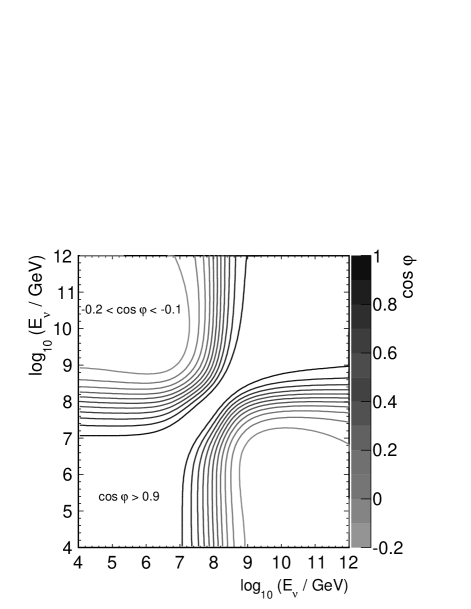
In Fig. 7, we plot $\cos{\varphi}$ for all energy pairs in the range $10^{4}-10^{12}$ GeV for charged current $\nu N$ cross sections. The analogous plots for $\bar{\nu}N$ and neutral current cross sections look similar. There are very strong correlations among cross sections at energies above $10^{9}$ GeV, and then again below $10^{7}$ GeV, with little correlation between energies in different regions. There are three reasons for this, all associated with the fact that in the lower energy region the cross section has a high proportion of its contribution from $x\sim 0.01$ or above, while in the higher energy region most of the contribution is from $x$ values lower than this. First, from sum rules in the PDFs, there is a crossing point where changes in PDFs become anticorrelated, i.e. for any change the PDFs, they tend to increase below this $x$ and decrease above this $x$ or vice versa. For high energy scales this is at $x\approx 0.01$. Second, this also happens to be the $x$ where there is a very large amount of accurate HERA data also tending to fix the PDFs. Thirdly, $x=0.01$ is a transition point at which for higher $x$ the dominant contributions are from valence quarks but for lower $x$ the sea quarks dominate, which are gluon driven.

III Cross Section Constraints

III.1 Motivation

The upper (lower) bounds on the Standard Model $\nu N$ cross sections differ from the central values by more than approximately 20% (15%) for neutrino energies above $10^{9}$ GeV. Above $10^{10}$ GeV, the uncertainties are more than approximately 50% (30%). We would like to constrain the cross sections at the highest energies because in that region neutrino experiments could be sensitive to new physics scenarios. Fortunately, there is a near guaranteed flux of neutrinos in the UHE energy regime from GZK interactions, but this so-called “cosmogenic” neutrino flux has large theoretical uncertainties associated with it.

Here we outline a technique Connolly (2006) to constrain the UHE $\nu N$ cross sections that is independent of the incident neutrino flux through the measured zenith angle distributions with a subterranean detector such as IceCube, ARA or ARIANNA Achterberg et al. (2006); Hoffman (2010); Gerhardt et al. (2010). The latter two experiments are currently in the first stages of deploying prototype detectors and will be focused on the UHE regime. Here, we focus on the ARA detector as an example, but our results are general to any subterranean neutrino detector with similar capabilities in energy measurement and reconstruction.

The sensitivity of neutrino detectors to $\nu N$ cross sections due to earth absorption has been addressed elsewhere in varying degrees Kusenko and Weiler (2002); Hooper (2002); Anchordoqui et al. (2010, 2006b, 2006c); Borriello et al. (2008); Romero and Sampayo (2010); Hussain et al. (2006, 2008). This is the only study that uses the full zenith angle distribution in the UHE regime to make hard predictions for the expected constraints on models with extra dimensions.

We note a few assumptions made for this study. First, we assume the incident flux is entirely neutrinos with no anti-neutrino component. Above $10^{8}$ GeV, the cross sections for neutrinos and anti-neutrinos differ by no more than about 6%. Second, we assume that all of the interactions occur at the same depth, $d=250$ m, and that it is precisely known. In an actual data analysis one would modify the $dn/d\cos{\theta_{z}}$ distributions so that $d$ is the measured depth, just as we use the measured energy for each event. The three-dimensional vertex resolution of the ARA detector is expected to be of order 10’s of meters. One can show that a depth uncertainty given by $\delta d$ changes $dP/d\cos{\theta_{z}}$ by a fraction of order $\delta d/L$. This only approaches of order 10% at the highest cross sections probed in this paper, approximately $10^{-28.5}$ cm². We also assume that the detector efficiency is flat in zenith angle $\theta_{z}$ and that the neutrino flux is isotropic. An analysis would fold in the measured detector efficiency, and neutrinos from any discovered sources could be removed from the sample. Finally, we assume that the energy resolution $\Delta\log_{10}E_{\nu}=0.4$, which is dominated by the uncertainty in inelasticity, is appropriate for both neutrino and black hole interactions.

III.2 ARA

The Askaryan Radio Array (ARA) is a nascent neutrino detector near the South Pole. It is an array of radio antennas deployed deep in the ice, designed to measure the radio Cerenkov pulse from UHE neutrinos Askaryan (1962, 1965); Alvarez-Muniz and Zas (1997); Saltzberg et al. (2001). If expanded to become a precision measurement, observatory class array of 300 to 1000 km² area, ARA will be capable of measuring hundreds of cosmogenic neutrinos per year. The first ARA testbed station was deployed in the 2010–2011 austral summer and the first ARA stations will be deployed in 2011-2012.

For the purpose of generating mock ARA data for this study, we use energy-dependent relative effective areas (the overall scale is not used) derived by inverting the projected flux limits for a 37-station array in Hoffman (2010). The stations are arranged on a triangular grid with the array forming a hexagon. Each station is made of three “strings” deployed vertically in the ice, each holding two pairs of vertically and horizontally polarized antennas that sit at 200 m depth, for a total of 12 antennas per station. The trigger requires 5 out of 12 stations measure a pulse that exceeds 3.5 times the expected noise level. We assume an energy resolution of $\Delta\log_{10}{E_{\nu}}=0.4$. The resolution on the neutrino $\theta_{z}$ is expected to be approximately $2^{\circ}$ for the events (approximately 80%) detected by one station only Gorham .

Our projected constraints will not depend on the exact size of the ARA detector. This is because the expected limits will be quoted for a specific number of neutrino events measured in the detector, whether that came from a weak flux measured with a large detector or a strong flux measured with a smaller detector. Nor do the projected constraints depend strongly on the energy threshold of the experiment, as long as there is at least a crude energy measurement capability. We will quantify these statements at the conclusion of Section III.5. In addition, our conclusions are not specific to the ARA experiment, and would be qualitatively similar for any subterranean detector with sensitivity to UHE neutrinos.

III.3 A Flux-Independent Technique for Measuring the UHE Neutrino-Nucleon Cross Section

Consider a neutrino (see Figure 8) that interacts in a subterranean detector such as ARA at depth $d$ and zenith angle $\theta_{z}$, the angle from vertical of the direction of origin of each incident neutrino. The neutrino travels a distance $D$ through the earth of radius $R$ before reaching its interaction point. From Figure 8 and using the law of sines,

$$\frac{\sin{\phi_{1}}}{R-d}=\frac{\sin(\pi-\theta_{z})}{R}.$$ (21)

which gives

$$\sin{\phi_{1}}=\frac{R-d}{R}\sin{\theta_{z}}.$$ (22)

Then since $\phi_{2}=\pi/2-\phi_{1}$,

$$\sin{\phi_{2}}=\cos{\phi_{1}}=\sqrt{1-\sin^{2}{\phi_{1}}}=\sqrt{1-\left(\frac{R-d}{R}\right)^{2}\sin^{2}{\theta_{z}}}$$ (23)

Then the distance traveled through the earth by the neutrino is:

$$D=(D-x)+x=R\sin{\phi_{2}}+(R-d)\sin\left({\theta_{z}-\frac{\pi}{2}}\right)$$ (24)

Inserting Eq. 23 into Eq. 24 we find:

$$D=R\sqrt{1-\left(\frac{R-d}{R}\right)^{2}\sin^{2}{\theta_{z}}}+(R-d)\sin\left({\theta_{z}-\frac{\pi}{2}}\right)$$ (25)

Then, taking $d<<R$ and replacing $\sin{\theta_{z}}$ with $\sqrt{1-\cos^{2}{\theta_{z}}}$, we find

$$D=\sqrt{(R^{2}-2Rd)\cos^{2}{\theta_{z}}+2Rd}-(R-d)\cos{\theta_{z}}.$$ (26)

If the detection efficiency is uniform in $\theta_{z}$, then for a neutrino with energy $E_{\nu}$, the probability distribution in $\theta_{z}$ for a detected interaction is given by Gonzalez-Garcia et al. (2008):

$$\frac{dP}{d\cos{\theta_{z}}}\left(E_{\nu}\right)=A\cdot\exp{\left(-\frac{D}{L\left(E_{\nu}\right)}\right)}=A\cdot\exp\left(-\frac{\sqrt{(R^{2}-2Rd)\cos^{2}{\theta_{z}}+2Rd}-(R-d)\cos{\theta_{z}}}{L\left(E_{\nu}\right)}\right)$$ (27)

where $R$ is the radius of the earth, $A$ is a constant that sets the total probability to unity, and $L\left(E_{\nu}\right)$ is the interaction length for a neutrino of energy $E_{\nu}$ along its path through the earth, given by:

$$L\left(E_{\nu}\right)=\frac{M_{N}}{\sigma(E_{\nu})\left<\rho\right>_{\theta_{z}}}$$ (28)

where $M_{N}$ is the nucleon mass, $\sigma(E_{\nu})$ is the $\nu N$ cross section at energy $E_{\nu}$ and $\left<\rho\right>_{\theta_{z}}$ is the mean density averaged over the distance travelled by the neutrino at the given $\theta_{z}$. The expected $\theta_{z}$ distribution from a sample of $n$ measured neutrino interactions with measured energies $\tilde{E}_{\nu}^{i}$ will be the sum of $n$ different $(dP/d\cos{\theta_{z}})_{i}$, so that the resulting expected $\theta_{z}$ distribution is then given by:

$$\frac{dn}{d\cos{\theta_{z}}}_{\rm{exp}}=\sum_{i=1}^{n}A_{i}\cdot\exp\left(-\frac{\sqrt{(R^{2}-2Rd)\cos^{2}{\theta_{z}}+2Rd}-(R-d)\cos{\theta_{z}}}{L\left(\tilde{E}_{\nu}^{i}\right)}\right).$$ (29)

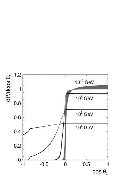
Note that due to the difference between measured neutrino energies $\tilde{E}_{\nu}^{i}$ and true energies $E_{\nu}^{i}$, the expected distribution will differ from the true one. In Fig. 9, we plot $dP/d\cos{\theta_{z}}$ for a few monoenergetic distributions. Notice the breaks in the distribution due to the neutrino trajectory intersecting the Earth’s core and mantle, derived using a simple three-layer model of the Earth’s interior. Due to this structure at lower energies, this technique could lead to a measurement of the Earth’s density profile with a km³ neutrino experiment such as IceCube that is independent of the traditional techniques used by geologists Gonzalez-Garcia et al. (2008).

Figure 8: Diagram showing neutrino incident on the earth used in derivation of Eq. 27.

Figure 9: Probability distributions in zenith angle for select neutrino energies. The width of each band is due to the cross section uncertainties reported in this paper. The kinks in the distributions at $\cos{\theta_{z}}=-0.1$ and $\cos{\theta_{z}}=-0.8$ are due to the neutrino paths reaching the earth’s mantle and core, respectively.

III.4 Models with Extra Space-Time Dimensions

There are a class of models for physics beyond the Standard Model that contain extra space-time dimensions Antoniadis et al. (1998); Arkani-Hamed et al. (1998); Anchordoqui et al. (2003); Alvarez-Muniz et al. (2002). These models are motivated by the need to resolve what is known as the Hierarchy Problem in particle physics, where the dramatically different energy scales for electroweak symmetry breaking and quantum gravity lead to a need for fine tuning of terms in the calculation of the Higgs mass.

In these extra-dimensional models (EDMs), the energy scale at which gravity dominates, $M_{D}$, is reduced to of order 1 TeV, just above the electroweak scale. The weakness of gravity in our 3+1 dimensional world is a consequence of its propagation in additional dimensions. The number of dimensions in the model beyond the four known space-time dimensions is denoted $N_{D}$.

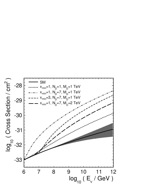
Interactions at energies at or above the reduced Planck mass lead to the production of micro-black holes, and this additional channel causes cross sections to be enhanced. The minimum black hole mass is given by $M_{\rm{BH}}^{\rm{min}}~{}=~{}x_{\rm{min}}M_{D}$, where $x_{\rm{min}}$ is a parameter in the model. Fig. 10 shows the predicted $\nu N$ cross sections for a few EDMs, from Alvarez-Muniz et al. (2002), compared to the SM cross sections calculated in this paper.

Tevatron experiments CDF and D0 have already set lower limits on $M_{\rm{D}}$ in the range of approximately 1-1.6 TeV with between 2 and 7 extra dimensions Aaltonen et al. (2008); Abazov et al. (2009). A recent paper by the CMS collaboration places constraints on black hole production at the LHC based on 35 pb^-1 of data at center-of-mass energy of 7 TeV Khachatryan et al. (2011). For $x_{\rm{min}}=1$, they exclude models with $n$ up to 6 for $1.5<M_{\rm{D}}<3.5$ TeV. They were not sensitive to models with $x_{\rm{min}}=3$ in the range of $M_{\rm{D}}$ considered. In addition, neutrino experiments have constrained UHE cross sections, but in a way that depends on a model for the neutrino flux Yoshida (2010). With the technique described here, neutrino experiments would be setting limits on EDMs that are competitive with collider experiments and independent of a flux model.

Figure 10: Cross sections for $\nu N$ interactions in models with extra space-time dimensions compared with the SM $\nu N$ cross sections. The gray band surrounding the SM cross sections are the uncertainties presented in this paper.

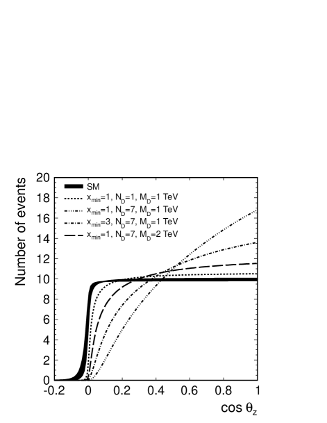
In Fig. 11, we plot the expected $\theta_{z}$ distribution for 100 events measured in ARA using cross sections from the SM compared to ones from a few select EDMs and a bin width of $\Delta\cos{\theta_{z}}=0.1$. The shape of the true energy spectrum of the 100 events is the product of an incident flux spectrum and an energy dependent effective area for the detector. Here we assume a neutrino flux from the GZK process as in Engel et al. (2001), and the ARA effective areas derived from Hoffman (2010) as described in Section III.2.

Figure 11: Predicted $\cos{\theta_{z}}$ distributions for 100 neutrino events observed by ARA for the SM and the four different EDMs shown in Figure 10.. The bin width is taken to be $\Delta\cos{\theta_{z}}=0.1$.

III.5 Projected Constraints

In order to assess the sensitivity of a future ARA detector to EDMs, we generate many pseudoexperiments, and compare the resulting pseudodata distributions to the predicted ones for the signal and null hypothesis respectively. For an expected number of events $N_{\rm{exp}}$, the number of events observed in a given pseudoexperiment is given by $n_{\rm{p}}$ and is Poisson distributed with mean $N_{\rm{exp}}$. The data in the $i^{\rm{th}}$ bin in $\cos{\theta_{z}}$ is denoted $n_{\rm{p},i}$. The mean number of events predicted in the $i^{th}$ bin centered on $\cos{\theta_{z}}=c_{0}$ is

$$\mu_{i}=\frac{dn_{\rm{p}}}{d\cos{\theta_{z}}}\left(c_{0}\right)\cdot\Delta\cos{\theta_{z}}$$ (30)

where $dn_{\rm{p}}/d\cos{\theta_{z}}$ is constructed for each pseudoexperiment using Equation 29. Note that through the $L(\tilde{E}_{\nu}^{i})$’s in Equation 29, $dn_{\rm{p}}/d\cos{\theta_{z}}$ depends on the model hypothesis, whether that be the SM or an EDM. Also note that we only use the measured energies, selected from the incident flux spectrum and then smeared according to detector resolution of $\Delta\log{E_{\nu}}=0.4$. The bin width is $\Delta\cos{\theta_{z}}=0.1$, or $\Delta\theta_{z}\approx 5.7^{\circ}$, which is greater than the expected resolution of the ARA array in $\theta_{z}$.

We use the following ratio of Poisson probabilities to discriminate between the two hypotheses Casal Larana :

$$Q=\frac{P_{\rm{poiss}}(\rm{data}~{}|~{}\rm{EDM~{}truth})}{P_{\rm{poiss}}(\rm{data}~{}|~{}\rm{SM~{}truth})}$$ (31)

where

$$P_{\rm{poiss}}(\rm{data}~{}|~{}\rm{EDM~{}truth})=\prod_{i=1}^{N}\frac{\mu_{\rm{EDM},i}^{n_{i}}e^{-\mu_{\rm{EDM},i}}}{n_{i}!}$$ (32)

and

$$P_{\rm{poiss}}(\rm{data}~{}|~{}\rm{SM~{}truth})=\prod_{i=1}^{N}\frac{\mu_{\rm{SM},i}^{n_{i}}e^{-\mu_{\rm{SM},i}}}{n_{i}!}.$$ (33)

Here, $N$ is the number of bins, and $n_{i}$ is the number of events measured in the $i^{th}$ bin. The number of events expected in a bin from an extra-dimensional model is $\mu_{\rm{EDM}}$ and the number expected in the Standard Model is $\mu_{\rm{SM}}$. Then, we find

$$-2\ln{Q}=-2\left[\sum_{i=1}^{N}n_{i}\ln\left({\frac{\mu_{\rm{EDM},i}}{\mu_{\rm{SM},i}}}\right)-\mu_{\rm{EDM},i}+\mu_{\rm{SM},i}\right]$$ (34)

The parameters for the EDM models are defined in Section III.4. Equation 34 is evaluated separately for pseudodata $\vec{n_{\rm{p}}}$ generated assuming SM and EDM truths, giving a different $-2\ln{Q}$ distribution for each. According to the Neyman-Pearson lemma, this likelihood ratio is the test statistic with the most discriminating power Neyman and Pearson (1933).

We estimate the constraints on EDMs expected to be set by the full scale ARA detector described in Section III.2 depending on the observed number of events $n_{\rm{p}}$. For the expected limit, we first consider the median value $-2\ln{Q}_{50}$ of the $-2\ln{Q}$ distribution from SM pseudoexperiments. The subscript denotes the percentage of SM pseudoexperiments with lower values of $-2\ln{Q}$. Then, for a given EDM model, the $p$ value is the fraction of EDM pseudoexperiments with $-2\ln{Q}<-2\ln{Q}_{50}$. Then, on average we can expect that a model can be excluded with percentage confidence level $CL=100\times(1-p)$.

The observed limit will differ from that expected due to fluctuations in the data, as reflected by the width of the $-2\ln{Q}$ distribution for SM pseudoexperiments. Therefore, we quote a range for the expected $CL$s by calculating $p$ values for $-2\ln{Q}_{16}$ and $-2\ln{Q}_{84}$, so that 68% of pseudoexperiments would give confidence levels in the range. Fig. 12 shows the distributions in $-2\ln{Q}$ for the SM and one EDM hypothesis, for 100 events observed in ARA. We mark the points along the abscissa $-2\ln{Q}_{16}$, $-2\ln{Q}_{50}$ and $-2\ln{Q}_{84}$.

Figure 12: Comparison of likelihood ratio $-2\ln{Q}$ from $N_{\rm{P}}$ pseudoexperiments generated assuming SM and EDM truth. The region between $-2\ln{Q}_{16}$ and $-2\ln{Q}_{84}$ contains 68% of the SM pseudoexperiments, with the median at $-2\ln{Q}_{50}$.

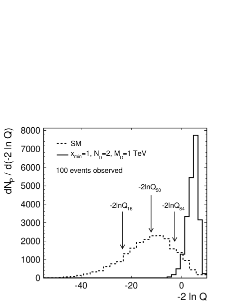
Fig. 13 shows the expected CLs for constraining EDMs as a function of the number of events observed with ARA. The black bands show the variation in the expected constraints brought about by the uncertainties on the SM cross sections presented here. The gray bands show the range of expected limits due to variations in the data; sixty-eight percent of the pseudoexperiments give constraints that lie in the gray region. The gray bands are centered on the curve corresponding to the central value standard model cross sections. Conservatively taking the SM upper bounds to be the true cross sections, for 100 events observed with ARA, the mean expectation is to exclude the following models: $x_{\rm{min}}~{}=~{}1,~{}M_{\rm{D}}=1,~{}N_{\rm{D}}\geq 2$; $x_{\rm{min}}~{}=~{}3,~{}M_{\rm{D}}=1,~{}N_{\rm{D}}\geq 3$; $x_{\rm{min}}~{}=~{}1,~{}M_{\rm{D}}~{}=~{}2,~{}N_{\rm{D}}\geq 3$. For $x_{\rm{min}}~{}=~{}3,~{}M_{\rm{D}}~{}=~{}2$, 110 events would be needed to be predicted to exclude $N_{\rm{D}}=7$.

Figure 13: Predicted confidence levels for excluding selected EDMs with an ARA experiment, depending on the number of events observed. The upper (lower) edges of the black bands in the figure show the range of expected limits taking the SM cross section to be their lower (upper) bounds as presented in this paper. The gray bands show the uncertainty due to pseudoexperiment statistics, with 68% of experiments expected to result in limits that lie within the gray region (using the central values for the SM cross section as the true cross sections).

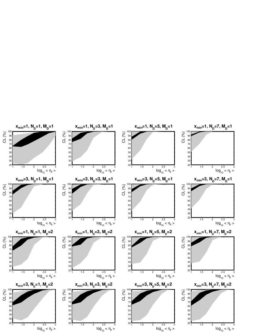
We have checked that these projected limits are robust to changes in the neutrino spectrum as well as details of the sensitivity of the experiment. We have calculated the expected constraints with an $E^{-3}$ neutrino spectrum, and also after shifting the ARA effective areas up and down in energy by a factor of 3. All of these changes have less of an effect on the expected constraints than the cross section uncertainties (the effect of which are depicted in the black bands of Fig. 13).

IV Conclusions

We have presented new calculations of the $\nu N$ and $\bar{\nu}N$, CC and NC cross sections in the neutrino energy range $10^{4}<E_{\nu}<10^{12}$ GeV using the MSTW 2008 PDFs, along with their PDF uncertainties. The cross section values are consistent with those reported in previous publications but the uncertainties presented here are significantly larger. This difference is due to a two-parameter model for the gluon parton distribution at very small $x$ used by MSTW 2008 arising from a fit to the global data, which leads to a wide range of allowed values for the gluon contribution at low-$x$. For ease of use in Monte Carlo simulations, we have provided parametrizations of the cross sections for each event type, the fraction of each type and the cross section uncertainty bounds in the energy range. In addition, we have outlined a procedure for generating $y$ values for a neutrino sample with $E_{\nu}\geq 10^{7}$ GeV using the Inverse Transform Method.

Finally, we present a technique for constraining UHE cross sections with a next-generation subterranean neutrino experiment. Using ARA as an example, we have shown that with 100 events observed, neutrino experiments set constraints on extra-dimensional models that are competitive with those set by collider experiments.