Band-phase-randomized Surrogates to assess nonlinearity in non-stationary time series

Abstract

Testing for nonlinearity is one of the most important preprocessing steps in nonlinear time series analysis. Typically, this is done by means of the linear surrogate data methods. But it is a known fact that the validity of the results heavily depends on the stationarity of the time series. Since most physiological signals are non-stationary, it is easy to falsely detect nonlinearity using the linear surrogate data methods. In this document, we propose a methodology to extend the procedure for generating constrained surrogate time series in order to assess nonlinearity in non-stationary data. The method is based on the band-phase-randomized surrogates, which consists (contrary to the linear surrogate data methods) in randomizing only a portion of the Fourier phases in the high frequency band. Analysis of simulated time series showed that in comparison to the linear surrogate data method, our method is able to discriminate between linear stationarity, linear non-stationary and nonlinear time series. When applying our methodology to heart rate variability (HRV) time series that present spikes and other kinds of nonstationarities, we where able to obtain surrogate time series that look like the data and preserves linear correlations, something that is not possible to do with the existing surrogate data methods.

I Introduction

The surrogate data method, initially introduced by J. Theiler et al. [1] is nowadays one of the most popular tests used in nonlinear time series analysis to investigate the existence of nonlinear dynamics underlying experimental data. The approach is to formulate a null hypothesis for a specific process class and compare the system output to this hypothesis. The surrogate data method can be undertaken in two different ways: Typical realizations are Monte Carlo generated surrogates from a linear model that provides a good fit to the data; constrained realizations are surrogates generated from the time series to fulfill the null hypothesis and to conform to certain properties of the data. The latter approach is suitable for hypothesis testing due to the fact that it does not requiere pivotal statistics [2]. In order to test a null hypothesis at a certain confidence level, one has to generate a given number of surrogates. Then, one evokes whatever statistic is of interest and compares the value of this statistic computed from the data to the distribution of values elicited from the surrogates. If the statistic value of the data deviates from that of the surrogates, then the null hypothesis may be rejected. Otherwise, it may not.
The linear methods for constrained realizations namely (i) Random shuffle (RS); (ii) Random phase (RP); and, (iii) Amplitude adjusted Fourier transform (AAFT) surrogates [1], were developed to test the null hypothesis that the data came from a (i) i.i.d gaussian random process, (ii) linear correlated stochastic process; and (iii) nonlinear static transformation of a linear stochastic process. Surrogates generated with the RS method are constrained to the amplitude distribution ($\mathcal{AD}$) or rank distribution of the original data, while the ones generated with the RP algorithm preserve the autocorrelation ($\mathcal{AC}(\tau)$) and surrogates generated with the AAFT algorithm preserve both the $\mathcal{AD}$ and $\mathcal{AC}(\tau)$ of the original data.
As the process that generates surrogate data is stationary [3], there could be some situations where surrogates fail to match the data, even though the $\mathcal{AD}$ and $\mathcal{AC}(\tau)$ are the same for the data and surrogates, so the null hypothesis could be trivially rejected. This is particulary true when data are non stationary. Because of this, when the statistical properties of data are time dependent it is not feasible to use the linear surrogate data methods for testing nonlinearity [4] (Timmer [5] showed that for some non-stationary processes the test is able to discriminate between linear and nonlinear data, but this is not a general result).
From the introduction of the linear surrogate data method, there has been a widespread interest in modifying it to assess nonlinearity in non-stationary time series. The first attempt (as we can tell) to apply the method to non-stationary time series was done by T. Schreiber [6]. He proposed that to deal with non-stationarity data, the null hypothesis should include it explicitly. Because otherwise, the rejection of a null hypothesis can be equally to nonlinearity or non-stationarity. e.g., given any process we can ask whether the data is compatible with the null hypothesis of a correlated linear stochastic process with time dependent local behavior. In order to answer this question in a statistical sense we have to create surrogate time series that show the same linear correlations and the same time dependency of the local behavior as the data and compare a nonlinear statistic between data and surrogates [4]. To generate surrogates constrained to data $\mathcal{AC}(\tau)$ and time dependence of local behavior, T. Schreiber [6] used an iterative procedure called simulated annealing. Unfortunately, this method requires a big amount of computational time and never became of popular usage.
In another study, A. Schmitz and T. Schreiber [7] proposed a different method to deal with non-stationarity. The proposed method involved dividing the signal into stationary segments, then applying the linear surrogate data method to each segment and finally joining the segments to form a surrogate time series of the same size as the original data. The major problem with this procedure is that there is not a straightforward way to find stationary segments in a non-stationary signal.
Recently, T. Nakamura and M. Small [8] proposed a new methodology to apply the surrogate data method to time series with trends, called Small Shuffle Surrogate (SSS) data method which is a modification of the RS algorithm. The main idea introduced in [8] is that in order to preserve the trend of the data in surrogates, the randomization should be applied only in a small scale, in this way all local correlations in the original time series are destroyed in surrogates; but the global behavior (i.e., the trend) is preserved.
Based on the idea of preserving the slow behavior of the signal in surrogates, T. Nakamura et al. [9] presented a modification of the RP algorithm which makes it suitable for data with trends. They called it the Truncated Fourier Transform Surrogate (TFTS) data method. TFTSs are constrained to conform to the $\mathcal{AC}(\tau)$ and with the correct parameter selection to the trend of data (the authors also apply the modification to the iAAFT method, thus preserving the $\mathcal{AD}$, $\mathcal{AC}(\tau)$ and the trend of data in surrogates). So, nonstationarities (in this case caused by the presence of a trend) are included in the null hypothesis, as suggested by A. Schmitz and T. Schreiber [6, 4]. The idea of the method is to preserve the slow behavior or trends while destroying all possible nonlinear correlations in the irregular fluctuations. To achieve this goal, the authors proposed to randomize phases only in the higher-frequency domain and not alter the low-frequency phases (the original idea of band-phase-randomized surrogates was briefly proposed by J. Theiler et al. [10] but it was not implemented until the work of T. Nakamura et al. [9]). This approach is in contrast to linear surrogate methods (RP and iAAFT), where all phases are randomized.
It is worth mentioning that other attempts have been made in order to assess nonlinearity in non-stationay data. L. Faes et al. [11] presented a method for calculating the parameters of an non-stationary AR model. Based on this method, they generated typical realizations of the non-stationary Heart Rate Variability (HRV) signals and tested for nonlinearity, but as the surrogates are typical realizations, one needs a pivotal statistic. Recently, C.J. Keylock [12] presented a modification of the iAAFT method based on the wavelet transform, with this method it is possible to generate surrogates constrained to preserve the $\mathcal{AC}(\tau)$ and the local mean and variance of the data, but according to our personal experience the method proposed by T. Nakamura et al. [9] is simpler to implement and achieves similar results. In a recent publication [13], we presented a modification of the TFTS through which we assessed nonlinearity in data with spikes, but this method is limited to data with gaussian $\mathcal{AD}$.
In this document we introduce the band-phase-randomized surrogate methods in a rather organized way, we also present the algorithms to facilitate and promote the application of the method. In regards to the method, we present a discussion on the parameter selection and introduce some modifications to the parameter selection criteria in order to make the method suitable for different types of nonstationarities (not only trends). To test the proposed methodology we applied the test to several simulated time series with different dynamical properties. We also applied the methods to HRV signals of healthy patients. Finally we conclude.

II Background

Prior to introducing the current technology in surrogate data methods, it is vital to make one observation: Hypothesis testing, such as the surrogate data method, cannot be used to determine what the data is, only what the data is not [2]. That is; if after our comparison we cannot distinguish between data and surrogates, this may be simply because our selected statistic is inadequate. Conversely, if the data and surrogates are different, then we can sate, that, with a certain probability the data is not consistent with the corresponding null hypothesis.

II-A Surrogate data methods

II-A1 Linear surrogate data methods

Linear surrogate data were introduced to preclude a linear filtered noise source as the possible origin of experimental data. The algorithms, as stated earlier, generate surrogate data that fulfill the null hypothesis of IID noise; linearly filtered noise; and, a monotonic nonlinear transformation of linearly filtered noise. Hence, these techniques produce flawless linear data. The algorithms to generate such surrogates can be stated as follows [1].

RS

A surrogate time series $\{s_{t}\}$ is generated from the scalar time series data $\{x_{t}\}$ by randomly shuffling $\{x_{t}\}$. This process destroys all temporal correlations (which are not expected in a IID process) but maintains the same $\mathcal{AD}$.

RP

The surrogate $\{s_{t}\}$ is generated by taking the Fourier transform of the data, randomising the phases (replacing it by the phases of a random IID process of the same length as $\{x_{t}\}$), and taking the inverse Fourier transform. The surrogate therefore maintains the linear correlations of data but any nonlinear structure is destroyed.

AAFT

One first re-scales the data original time series so that it is Gaussian, then generates an Algorithm 1 surrogate of the data $\{p_{t}\}$, and finally re-orders the original data so that it has the same rank distribution as $\{p_{t}\}$. This re-ordered time series constitutes the surrogate $\{s_{t}\}$. This process achieves two aims: first, just as with the Algorithm 1, the power spectra (and therefore linear correlations) of data is preserved in surrogates; second, the re-ordering process means that the $\mathcal{AD}$ of data and surrogates are also identical.

It should be noted that the AAFT algorithm does not deliver what it promises. The phase randomisation will preserve the linear correlation, but re-scaling the output of the inverse Fourier transform $\{p_{t}\}$ to have the same $\mathcal{AD}$ as the original data will alter the autocorrelation structure of the data. Although the data and surrogate will have identical rank distribution, the linear correlation will only be approximately the same. A solution to this problem has been proposed by T. Schreiber and A. Schimitz [14]. Essentially, the solution is to iterate the AAFT algorithm until convergence is achieved. However, there is no guarantee that this iteration will, in fact, converge. This algorithm is refereed to as improved AAFT (for a discussion on the convergence of the iAAFT algorithm see [15]).

II-A2 Surrogate data methods for data with trends

As stated earlier, when data are non-stationary, the hypothesis addressed by the linear surrogate data methods are trivially rejected. Two different surrogate data methods have been proposed to tackle data with trends, the SSS and the TFTS data methods. The hypothesis tested by SSS algorithm is that the data, while possibly exhibiting some trend, is otherwise just noise [8]; while the hypothesis tested by TFTS algorithm is that the data, while possibly exhibiting some trend, is generated by a stationary linear system [9]. These algorithms can be stated as follow [16].

SSS

Let $\{i_{t}\}$ be the index of $\{x_{t}\}$ (that is, $i_{t}=t$ and so $x_{i_{t}}=x_{t}$). Obtain $\{i^{\prime}_{t}\}=\{i_{t}+Ag_{t}\}$ where $\{g_{t}\}$ are Gaussian random numbers, and $A$ is an amplitude (note that $\{i_{t}\}$ will be a sequence of integres, whereas $\{i^{\prime}_{t}\}$ will not). Rank order $\{i_{t}\}$ to obtain $\{r_{t}\}$. The surrogates $\{s_{t}\}$ are obtained from $s_{t}=x_{r_{t}}$. If $A$ is an intermediate value (e.g. 1), surrogates generated by this algorithm will preserve the slow trend in the data, but any inter-point dynamics will be destroyed by the local shuffling of individual points.

TFTS

The surrogate $\{s_{t}\}$ is generated by taking the Fourier transform of the data $\{X_{\omega}\}_{\omega}$. Then generating random phases $\phi_{\omega}$, such that $\phi_{\omega}\sim U(0,2\pi)$ if $\omega>f_{c}$ and $0$ if $\omega\leq f_{c}$ ( $\phi_{\omega}$ have to be antisymmetric around $\phi_{0}$). Finally taking the inverse Fourier transform of the complex series $\{X_{\omega}e^{\imath\phi_{\omega}}\}_{\omega}$ (Fig. 1). As in the RP surrogates, all linear dependencies are preserved in surrogates. But, since some phases are untouched, TFTS data may still have nonlinear correlations. However, it is possible to discriminate between linear and nonlinear data because the superposition principle is only valid for linear data, so when data are nonlinear, even if the power spectrum is preserved completely, the inverse Fourier transform data using randomized phases will exhibit a different dynamical behavior

Figure 1: Flow chart of the Truncated Fourier Transform Surrogate method.

TFTSs are influenced primarily by the choice of frequency $f_{c}$. If $f_{c}$ is too high, surrogates are almost identical to the original data. In this case, even if there is nonlinearity in the data, one may fail to detect it. Conversely, if $f_{c}$ is too low, surrogates are almost the same as the linear surrogate and the local behavior is not preserved. In this case, even if there is no nonlinearity in the data, one may wrongly judge otherwise.
In general, the correct value of $f_{c}$ cannot be determined a priori. To select an adequate value of $f_{c}$, T. Nakamura et al. [9] proposed to start randomizing a portion of the higher frequency domain (e.g. a 1$\%$ of the higher frequency domain, i.e., $f_{c}\approx N/2$), decreasing $f_{c}$ until the data linearity is no longer preserved in the surrogates (i.e., $\mathcal{AC}(\tau=1$) of data falls outside the distribution of surrogates) and then perform the test with the last value of $f_{c}$ for which linearities of data are preserved in surrogates.

II-B Significance and power of the test

Applying a statistical hypothesis test to observed data can result in two outcomes: either the null hypothesis is rejected, or it is not. In the former case there is a probability $\alpha$ that the null hypothesis is rejected even though it is true (Type I Error), in the latter case there is a probability $\beta$ (Type II Error) that we will fail to reject the null when it is in fact false. The probability $\alpha$ is known as the significance level, its complement ($1-\alpha$) is the confidence level. For example, if one generates 19 surrogates using some algorithm, and these yield a larger (or smaller) value of some statistic than the data, then the probability that this result occurred by chance is $\alpha=\frac{1}{20}$, and hence we conclude at the 0.05 significance (0.95 confidence) level for a one-sided test that the selected statistic is different from the surrogates. Conversely, the power of a test ($1-\beta$) is the probability the null hypothesis is correctly rejected.
Clearly, the probability $\alpha$ is determined by the number of trials and the number of independent test statistics. Computing $\alpha$ is only a matter of computing probabilities. The problem is that the value of $\beta$ is not clear. The actual power $\beta$ will depend on the choice of test statistic. If the test statistic is independent of data and surrogates then the power is determined by the number of trials [16].

III Nonlinearity test for non-stationary time series: Physiological data approach

III-A Database

III-A1 Simulated time series

To test the proposed methodology we applied it to different simulated time series, two linear (stationary and non-stationary) and two nonlinear (stationary and non-stationary). The linear time series were generated by the following AR(2) process [5]

$$x(n)=a_{1}(n)x(n-1)+a_{2}x(n-2)+\eta.$$ (1)

Where

$$\begin{split}a_{1}(n)&=2cos(2\pi/T(n))e^{(-1/\tau)},\ a_{2}=e^{(-2/\tau)},\\ T(n)&=T_{e}+M_{T}sin(2\pi t/T_{mod}),\\ \eta&\sim\mathcal{N}(0,1).\end{split}$$ (2)

To generate a linear stationary signal we used $T_{e}=10$, $T_{mod}=250$, $\tau=50$ and $M_{T}=0$, for the linear non-stationary signal we used $M_{T}=6$.
The nonlinear time series were generated by the following nonlinear process [17]

$$x(n)=a_{1}(n)x(n-1)(1-x^{2}(n-1))e^{(-x^{2}(n-1))}+a_{2}x(n-2).$$ (3)

For the nonlinear stationary signal we used $a_{1}(n)=3.4$ and $a_{2}=0.8$. For the nonlinear non-stationary signal we used

$$a_{1}(n)=\begin{cases}3.0&\text{if $0<n\leq N/2$,}\\ 3.4&\text{if $N/2<n\leq N$.}\end{cases}$$

Figure 2: a) Linear stationary (LS) signal, b) linear non-stationary (LNS) signal, c) nonlinear stationary (NLS) signal and d) nonlinear non-stationary (NLNS) signal.

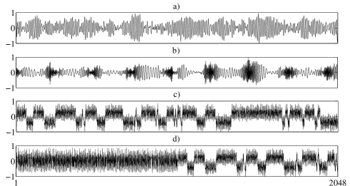
An example of each of these signals is shown in Fig. 2 with $N=2048$.

III-A2 Physiological time series

The HRV time series of healthy subjects were extracted from the MIT-BIH Normal Sinus Rhythm Database in Physionet [18, 19] according to annotations for only normal beats. Sample rate was 128 Hz in 24-hr Holter recordings.

III-B Proposed procedure

It is widely accepted that most biomedical systems are dynamic and produce nonstationary signals [20]; the presence of slow varying trends is only one type of nonstationarities present in physiological signals. So, the novelty of the present document is to propose a methodology based on the TFTS data method (which from now on will be called band-phase-randomized surrogate data method) that allows us to assess nonlinearity in data with different kinds of nonstationarities (e.g., spikes, abrupt changes in the dynamical behavior). The proposed procedure is depicted in Fig 3.

Figure 3: Proposed methodology to assess nonlinearity in non-stationary time series.

III-B1 Band-Phase-Randomized Surrogates

Band-phase-randomized surrogate data method is, as mentioned, a modification of the RP algorithm in which not all phases but a portion of the phases in the high-frequency band are randomized.
Unfortunately, as stated by [10] it is difficult to automate the procedure in order to make it applicable to all time series. The methodology proposed in [9] to find de correct value of $f_{c}$ (i.e., the correct portion in the frequency band in which the phases are to be randomized) is only useful when data have a slow varying trend, because when this statement is not true, the stoping criterium is never met (i.e., $\mathcal{AC}(\tau=1$) of data falls outside the distribution of surrogates ) and so one always ends up using the iAAFT algorithm even when data is not-stationary. In [13], we propose that the stoping criterium should be the similarity between data and surrogates, i.e., surrogates should preserve the local behavior of the data. But, when the data is in fact nonlinear this criterium fails. Next, we present a new method for selecting the correct parameter of the algorithm.

It should be noted that the use of the end-phase-randomized surrogate data method will not improve the type II error because if the method fails to reject the null when all phases are randomized (using some statistic) then it certainly will not be able to reject the null when just a portion of the phases are randomized. On the other hand, the type I error will be improved by means of this method.

Figure 4: a) FT magnitude (note the logarithmic scale) and b) FT phases as a function of $n$ for LS signal with $N=1940$ (continuos line) and one Band-Phase-Randomize surrogate $f_{c}=291$ (dotted line). $S(n)$ for data and surrogates are equal for all $n$, but $\phi(n)$ is equal only for $n\leq f_{c}$. In this case we are randomizing 70$\%$ of the higher frequency domain. In b) the difference between the FT phases of data and surrogates is displaced form cero for clarity.

III-B2 Parameter selection

To overcome the parameter selection problem we propose not to use just one value of $f_{c}$ but a set of values. The proposed methodology is as follows: First, we select two values $f_{c_{max}}\approx N/2$ and $f_{c_{min}}$. Within this range, we select a set of values for $f_{c}$ (e.g., 10 values), then we generate Band-Phase-Randomized Surrogates using all those values and finally we perform the nonlinearity test (one must ensure that linear correlations of the data are preserved in surrogates for those values of $f_{c}$).
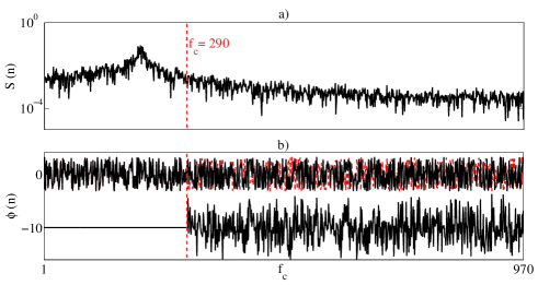
There are several ways to determine the value $f_{c_{min}}$; if the Fourier transform magnitude ($S(n)$) has a pronounced peak then, $f_{c_{min}}$ is selected above the peak (see Fig. 4 a)). If $S(n)$ does not have a pronounced peak (or has several) then $f_{c_{min}}$ should be selected as the lowest value for which the local mean of the data is preserved in the surrogates (see Fig. 5); when data have a pronounced peak, both criteria result in a similar value of $f_{c_{min}}$.

III-C Selection of the discriminant statistic

Dynamical measures are often used as discriminating statistics, the correlation being dimension one of the most popular choices [16]. To estimate these, we first need to reconstruct the underlying attractor. For this purpose, a time-delay embedding reconstruction is usually applied. But this method is not useful for data exhibiting nonstationarities because at the moment, there is no optimal method for embedding such data [21].
Therefore, as discriminant statistics we chose the Average Mutual Information ($\mathcal{I}(\tau)$) [21]. The $\mathcal{I}(\tau)$ is a nonlinear version of the $\mathcal{AC}(\tau)$. It can answer the following question: On average, how much does one learn about the future from the past? So, we expect that if our data is not just a realization of a linear non-stationary noisy process it would have a larger $\mathcal{I}(\tau)$ than that of the surrogates.

III-D Implementation

Prior to the application of the methodology, we normalize the data to zero mean and unit variance and find the largest sub-segment that minimizes the end-point mismatch (this step is extremely important and can be done automatically as suggested in [4]); if the data have a trend then one can apply the preprocessing methodology proposed in [9].
In order to reject a null hypothesis we generate $M=99$ surrogates using an improved Amplitude Adjusted version of the band-phase-randomized surrogate data method, because as the $\mathcal{I}(\tau)$ depends on the data $\mathcal{AD}$, we have to generate surrogates with equal $\mathcal{AD}$ as the data to avoid false rejections. Then we compute the $\mathcal{I}(\tau=1)$ for the ensemble of surrogates and for the original time series (in a previous study we showed that $\mathcal{I}(\tau)$ is sensible to the type of dynamics only for small lags [22]). If $\mathcal{I}(\tau=1)$ is greater than that of the surrogates we reject the null hypothesis at the 0.01 significance level; otherwise, we do not reject the null.

IV Results

IV-A Numerical results

Figure 5: Normalized rms difference between local mean (continuos line) and variance (dotted line) of data (a) LS signal, b) LNS signal, c) NLS signal and d) NLNS signal) and Band-Phase-Randomize surrogates as a function of $f_{c}$. The local mean and variance was calculated using windows of length 64 with 50$\%$ overlap.

Prior to testing for nonlinearity we normalized each time series to zero mean and unit variance, and selected a subsegment of the signals that minimized the end-point mismatch, we end up with N= 1940, 1954, 1996 and 2023 number of data points for each time series.
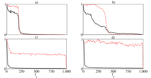
Fig 5 shows the normalized root mean square (rms) difference between data (a) LS signal, b) LNS signal, c) NLS signal and d) NLNS signal) and Band-Phase-Randomized surrogates as a function of $f_{c}$ (when $f_{c}=0$ Band-Phase-Randomized surrogates and the iAAFT surrogates are equivalent). It can be noted that for linear data it is possible to obtain surrogates with almost the same local behavior as the original time series while for nonlinear data the local variance of surrogates is never similar to the data (except for $f_{c}=N/2$). This result is expected because the variance is a nonlinear statistic and surrogates are only constrained to sample mean, sample variance $\mathcal{AD}$ and $\mathcal{AC}(\tau)$ of data.
From Fig. 5 we notice that $f_{c_{min}}\approx$ 280, 400, 50 and 50 for each time series. Anyhow, we use $f_{c_{min}}=0$ and $f_{c_{max}}=N/2-10$ for the following result.
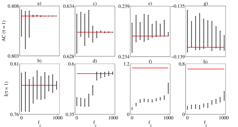
Fig. 6 shows the $\mathcal{AC}(\tau=1$) and $\mathcal{I}(\tau=1)$ from data and Band-Phase-Randomized surrogates. It can be noted that for linear stationary data (fig. 6 a) and b) ) the hypothesis tested by the iAAFT algorithm cannot be rejected ($f_{c}=0$) and as expected, randomizing only a portion of the higher frequency domain, does not affect this result. When data is nonlinear (stationary or not) the test rejects the null hypothesis of linearity for all values of $f_{c}$ within the selected range of values. As shown in fig. 6 g), $\mathcal{AC}(\tau=1)$ of data is not similar to that of surrogates for some values of $f_{c}$, this implies that linear correlations of the data are not well preserved in the surrogates and one should not perform the nonlinearity test for these values of $f_{c}$. In spite of this, the hypothesis is rejected.
The most interesting case (at least for the purpose of the present document) is the linear non-stationary case; in this situation nonlinearity is detected using the iAAFT algorithm (fig. 6 d), $f_{c}=0$), so a careless application of the linear surrogate data method would result in a false detection of nonlinearity (type I error). But, as shown in fig. 6 d), the nonlinearity is detected only for certain values of $f_{c}$, in this case when $f_{c}>500$ nonlinearity is no longer detected by the test (the same curve as fig. 6 d), is obtained when the value of $M_{T}$ in (2) is slightly modified, the range of values of $f_{c}$ for which the null is rejected vary with $M_{T}$).
Two other important aspects can be noticed in Fig. 6, first, it is remarkable that when local mean and variance of surrogates are similar to data, $\mathcal{AC}(\tau=1)$ of ensemble of surrogates is almost the same as data, this can be seen in Fig. 6 a) and c) for $f_{c}>300$ and $f_{c}>500$ respectively (compare this with the results shown in Fig. 5 a) and b)), but the same results are not observed when local variance of surrogates is not similar to data (although the local mean of surrogates is similar to data), this can be seen in Fig. 6 e) and g) respectively (compare this with the results shown in fig. 5 c) and d)). Second, besides differentiating between linear and nonlinear time series (stationary or not), this test can be used to discriminate between linear stationary and linear non-stationary data, in the former case the hypothesis of linearity will be accepted for all values of $f_{c}$, while in the latter this will occur only for certain values of $f_{c}$ (as shown in Fig. 6 d)).

Figure 6: (Color online) a), c), e) and g) $\mathcal{AC}(\tau=1$)of the original time series (a),b) LS signal, c),d) LNS signal, e),f) NLS signal and g),h) NLNS signal) (continuos vertical line) and $\mathcal{AC}(\tau=1$) of an ensemble Band-Phase-Randomize surrogates (5th, 50th and 95th percentiles) as a function of $f_{c}$ ($f_{c}=0$ is the result of using the iAAFT algorithm). b), d), f) and h) the same as above but using the $\mathcal{I}(\tau=1)$.

To test the robustness of the method we performed the same analysis presented here adding a 5$dB$ white noise to each time series and found similar results.

IV-B Application to HRV signals

Despite the fact that nonlinear dynamics are involved in the genesis of HRV as a result of the interactions among hemodynamic, electrophysiological, and humoral variables [23], there is no proof that the recorded HRV time series (usually derived from an ECG) reflects this nonlinearity, this must be proven in each case. In this section, we apply the proposed methodology to assess nonlinearity in HRV which are known to have spikes and nonstationarities due to variation of the patient activity (see Fig. 7 a).
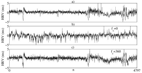
Fig. 7 a), shows a 1 hour record of the HRV of a healthy 32 year old male, the starting time is about midnight and the patient is at rest. Fig 7 b), depicted one surrogate time series generated using the classical method (iAAFT surrogates), while surrogates presented in Fig 7 c), where generated using the band-phase-randomized surrogate data method with $f_{c}=360$.
The original time series has much of its energy concentrated in the high frequency components, and as in the iAAFT surrogates the high frequency energy of the original time series is blurred in all the frequency spectrum, one gets surrogates that are not simular to the HRV signal, allowing a trivial rejection of the null hypothesis. Band-phase-randomized surrogates overcome this problem by preserving the phases in a portion of the frequency spectrum, in this way, high frequency and low frequency components of the original time series are preserved in surrogates, as can be seen in Fig. 7 a) and c).

Figure 7: a) Segment of a HRV time series of a 32 year old healthy male, b) surrogate generated using the iAAFT algorithm, c) band-phase-randomized surrogates using $f_{c}=360$.

Using the proposed methodology it was found that $f_{c_{min}}=200$ and $f_{c_{max}}=2300$, with this information, Fig. 8 was generated.

Figure 8: a) $\mathcal{AC}(\tau=1$), b)$\mathcal{I}(\tau=1)$ for the HRV signal and Band-Phase-Randomize surrogates as a function of $f_{c}$.

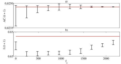
As expected, the null tested by the iAAFT surrogates is rejected ($f_{c}=0$), but as seen in Fig. 6 d), this is not an indicator of nonlinearity, but of nonlinearity or nonstationarity, and as in this case it is acknowledge that the tested signal is nonstatioanary, this test is not giving any new information about this signal. But the proposed methodology is; it can be noticed that when $f_{c}$ is within the selected range, the null hypothesis is always rejected (and the linear correlations of the original time series are always preserved in surrogates), and as was already noticed (Fig. 6 f) and h)), this is a clear indicator of the presence of nonlinear correlations. By this means, we confirm that there is a complex nonlinear physiological process underlying the HRV.

V Conclusion

In this document, we presented a methodology based on the TFTS data method and the iAAFT algorithm that allows us assess nonlinearity in non-stationary time series. Based on some simulated data we demonstrate that our methodology is able to differentiate between linear stationary, linear non-stationary (even when the linear data is transformed by a nonlinear monotonic static observation function) and nonlinear time series. This method is different from previously proposed nonlinearity tests because: i) we do not randomize the phases in all the frequency domain but in a portion of the frequency domain , and ii) we do not select a correct value of $f_{c}$ but a correct range $[f_{c_{min}},f_{c_{max}}]$, and within this range, a set of values for the parameter $f_{c}$.
Applying this test to physiological time series, we found that nonlinear correlations are present in HRV signals of a healthy male, this confirms that nonlinear dynamics are involved in the genesis of HRV, but as mentioned, every times series should be tested because there no a priori method to determine if a given signal represent the nonlinearity of the process.
It is worth mentioning that as pointed out by many authors ([9], [10]), the linear surrogate data methods are only suitable for stochastic like data, and as the present methodology is based on that, the same limitations apply.

References

- [1] J. Theiler, S. Eubank, A. Longtin, B. Galdrikian, and J. D. Farmer, “Testing for nonlinearity in time series: The method of surrogate data,” Physica D, vol. 58, p. 77 – 94, 1992.
- [2] J. Theiler and D. Prichard, “Constrained-realization monte-carlo method for hypothesis testing,” Physica D, vol. 94, no. 4, pp. 221 – 235, 1996.
- [3] D. T. Kaplan, Frontiers of blood pressure and heart rate analysis. Amsterdam: IOS Press, 1997, vol. 35, ch. Nonlinearity and Nonstationarity : The use of surrogate data in interpreting fluctuations, pp. 15 – 28.
- [4] T. Schreiber and A. Schmitz, “Surrogate time series,” Physica D, vol. 142, pp. 346–382, 2000.
- [5] J. Timmer, “Power of surrogate data testing with respect to nonstationarity,” Physical Review E, vol. 58, no. 4, pp. 5153 – 5156, 1998.
- [6] T. Schreiber, “Constrained randomization of time series data,” Physical Review Letters, vol. 80, no. 10, pp. 2015 – 2018, 1998.
- [7] A. Schmitz and T. Schreiber, “Surrogate data for non-stationary signals,” in Workshop on Chaos in Brain?, K. Lehnertz, J. Arnhold, P. Grassberger, and C. E. Elger, Eds. Singapore: World Scientific, 1999, p. 222–225.
- [8] T. Nakamura and M. Small, “Small-shuffle surrogate data: Testing for dynamics in fluctuating data with trends,” Physical Review E, vol. 72, pp. 056 216–1 – 056 216–6, 2005.
- [9] T. Nakamura, M. Small, and Y. Hirata, “Testing for nonlinearity in irregular fluctuations with long-term trends,” Physical Review E, vol. 74, pp. 026 205–1 – 026 205–8, 2006.
- [10] J. Theiler, P. S. Linsay, and D. M. Rubin, “Detecting nonlinearity in data with long coherence times,” in Predicting the future and understanding the past. Addison-Wesley, 1993, pp. 429–455.
- [11] L. Faes, H. Zhao, K. H. Chon, and G. Nollo, “Time-varying surrogate data to assess nonlinearity in nonstationary time series: Application to heart rate variability,” IEEE Trans. on Biomedical Engineering, vol. 56, no. 3, pp. 685 – 695, 2009.
- [12] C. J. Keylock, “A wavelet-based method for surrogate data generation,” Physica D, vol. 225, p. 219–228, 2007.
- [13] D. Guarín, A. Orozco, E. Delgado, and E. Guijarro, “On detecting determinism and nonlinearity in microelectrode recording signals: Approach based on non-stationary surrogate data methods,” in 32nd Annual International Conference of the IEEE EMBS, 2010, pp. 4032 – 4035.
- [14] T. Schreiber and A. Schmitz, “Improved surrogate data for nonlinearity tests,” Physical Review Letters, vol. 77, p. 635 – 638, 1996.
- [15] V. Venema, F. Ament, and C. Simmer, “A stochastic iterative amplitude adjusted fourier transform algorithm with improved accuracy,” Nonlinear Processes Geophysics, vol. 13, p. 321–328, 2006.
- [16] M. Small, T. Nakamura, and X. Luo, Nonlinear Phenomena Research Perspectives. Nova Science Publications, 2007, ch. Surrogate data methods for data that isn’t linear noise, pp. 55 – 81.
- [17] L. Faes, H. Zhao, K. H. Chon, and G. Nollo, “A method for the time-varying nonlinear prediction of complex nonstationary biomedical signals,” IEEE Trans. on Biomedical Engineering, vol. 56, no. 2, pp. 205 – 209, 2009.
- [18] L. Glass, “Introduction to controversial topics in nonlinear science: Is the normal heart rate chaotic?” Chaos, vol. 19, pp. 028 501–1 – 028 501–4, 2009.
- [19] A. L. Goldberger, L. A. N. Amaral, J. M. H. L. Glass, P. C. Ivanov, R. G. Mark, J. E. Mietus, G. B. Moody, C.-K. Peng, and H. E. Stanley, “Physiobank, physiotoolkit, and physionet : Components of a new research resource for complex physiologic signals,” Circulation, vol. 101, pp. 215 – 220, 2000.
- [20] R. M. Rangayyan, Biomedica Signal Analysis, M. Akay, Ed. IEEE Press, 2002.
- [21] M. Small, Applied Nonlinear Time Series Analysis - Applications in Physics, Physiology and Finance. World Scientific, 2005.
- [22] D. Guarín and A. Orozoco, “Pruebas de no linealidad para series temporales,” Submited, 2010.
- [23] T. F. of The European Society of Cardiology, T. N. A. S. of Pacing, and Electrophysiology, “Heart rate variability. standards of measurement, physiological interpretation, and clinical use,” European Heart Journal, vol. 17, pp. 354 – 381, 1996.