How does the first water shell fold proteins so fast ?

Abstract

First shells of hydration and bulk solvent plays a crucial role in the folding of proteins. Here, the role of water in the dynamics of proteins has been investigated using a theoretical protein-solvent model and a statistical physics approach. We formulate a hydration model where the hydrogen bonds between water molecules pertaining to the first shell of the protein conformation may be either mainly formed or broken. At thermal equilibrium, hydrogen bonds are formed at low temperature and are broken at high temperature. To explore the solvent effect, we follow the folding of a large sampling of protein chains, using a master-equation evolution. The dynamics shows a clear mechanism. Above the glass-transition temperature, a large ratio of chains fold very rapidly into the native structure irrespective of the temperature, following pathways of high transition rates through structures surrounded by the solvent with broken hydrogen bonds. Although these states have an infinitesimal probability, they act as strong dynamical attractors and fast folding proceeds along these routes rather than pathways with small transition rates between configurations of much higher equilibrium probabilities. At a given low temperature, a broad jump in the folding times is observed. Below this glass temperature, the pathways where hydrogen bonds are mainly formed become those of highest rates although with conformational changes of huge relaxation times. The present results reveal that folding obeys a double-funnel mechanism.

To this date, the three-stranded $\beta$ sheet is the faster folder finding its native structure in the amazingly short time of 140 nano-seconds Xu et al. (2006). The protein folding problem is still considered as one of the major unsolved problems of science Sci (2005) and the answer to the Levinthal question Levinthal (1968) ”how a protein can fold so fast ?” remains a ”grand challenge” Dill et al. (2007).

Protein folding is the process whereby a protein folds into its native structure. The slowest folding proteins may require a few minutes due among other factors to proline isomerization Kim and Baldwin (1990). They fold passing through many intermediate states. On the other hand, many small single-domain proteins fold very rapidly over time scales of a few microseconds Jackson (1998); Kubelka and Hofrichter (2004). For many of these proteins, the folding process is a single exponential function of time Jackson (1998); Kim and Baldwin (1990) and is modeled by a two-state mass action model and an Arrhenius diagram on which the free energy of some ensembles of chain conformations is plotted as a function of reaction coordinate, usually not known. This diagram exhibits a transition state between the unfolded and the native states Schonbrun and Dill (2003).

Moreover, some ultra fast folders exhibit more complex kinetics with non-Arrhenius behavior Ghosh et al. (2007) (i.e. non-linear dependence of the logarithm of the folding rate on the inverse of the temperature). Some results show that the activation energy is positive at room temperature, decreases as the temperature increases and may become negative at high temperature Zhu et al. (2003). It has been suggested that this could arise from the temperature dependence of the hydrophobic effect Chan and Dill (1998a); Akmal and Muñoz (2004).

An alternative to this transition-state view is the concept of folding funnel Leopold et al. (1992). This energy-landscape picture is based on the idea of minimal frustration Bryngelson et al. (1995), which states that the evolutionary mechanism has retained those protein sequences that have a funnel-like energy landscape. In that concept, the height of the funnel represents the conformational energy and its width represents the entropy of the subset of chain conformations of a given energy Onuchic et al. (1996); Wolynes (1997); Socci et al. (1998); Onuchic and G. (2004); Clark (2004). The top of the funnel is populated by the huge number of denaturated configurations with a large energy and entropy and the bottom with the unique native structure of very low energy and quasi-nil entropy. Each protein chains folds from the top of the funnel towards the bottom.

The transition-state theory and the folding-funnel picture are two different approaches. The first one describes well the two-state kinetics, but does not explain why folding is so fast. The second one explains well why folding is so fast, and the thermodynamic free energy barrier, that gives rise to two-state kinetics and makes transition-state theory applicable to the folding process, is essentially of entropic nature.

Lattice models of proteins are among the favorite tools for the theoretical study of folding. The microscopic representation of the proteins is simplified to allow large sampling of the configurational space. Proteins are modeled as self-avoiding-walk chains of beads, which are located on a two or three-dimensional square or cubic lattice. For small-length chains, a full enumeration of the conformations allows the exact calculation of the partition function, and, thus of statistical averages Lau and Dill (1989); Gõ (1983); Dinner et al. (1994); Collet (2001). The Hamiltonian of a given conformation of the chain results from the interaction of the first neighbors of the beads on the lattice, but not in the sequence. The more popular model of couplings between monomers are known as the GõGõ (1983), the HP Lau and Dill (1989); Chan and Dill (1991, 1994, 1998b) and the random-energy model(REM) Derrida (1981); Shakhnovich and Gutin (1990); Šali et al. (1994a, b); Gutin et al. (1995a, b). In the Gõ model, the interaction between the beads of a given compact structure, chosen as the native conformation, is set to -1 and all the other couplings to 0. In the HP model, the sequence of the protein is given in terms of a series of hydrophobic (H) or polar (P) residues and the coupling between two hydrophobic beads is set to -1 and that involving at least one polar monomers to 0. In the REM, a matrix of couplings between all pairs of residues is constructed by drawing random numbers from a Gaussian distribution.

Despite the numerous results obtained with such models, they fail to reproduce a fundamental feature of a protein : its cold denaturation. This mechanism is associated to the loss of stability of the native structure upon cooling down the system Privalov (1990); Nishi et al. (1994); Kumar et al. (2006). For half a century, it has been well known that water plays a crucial role in the mechanism of folding Kauzmann (1959); Warshel and Lifson (1970); Dill (1990) and an understanding of cold denaturation requires a finer model of the solvent than the temperature-independent attractive parameters used in Gõ, HP or REM. Some recent refinements of the models, including temperature dependence of the hydrophobic effect, have allowed to model the cold transition De Los Rios and Caldarelli (2000, 2001); Collet (2001, 2005) to be described.

As the physics of protein folding proceeds in water and the interactions of the protein chemical groups are solvent mediated, the representation of the solvent is of great importance Chan (2004). The hydrophobic effect is an active field of research by itself Garde et al. (1996); Hummer et al. (1998); Garde et al. (1999); Gomez et al. (1999); Lyndell-Bell and Rasaiah (1997). It represents the tendency of water to exclude nonpolar solutes. It results from a disruption of the network of hydrogen bonds between water molecules caused by the transfer of an nonpolar solute into water. The energy variation of this process is favorable at room temperature, whereas the entropy cost leads to a large positive free energy of transfer. In addition, the physics of the solvent-mediated interactions of the protein may be captured by studying the interaction of two nonpolar solutes immersed in water Chan (2004). This prototypical interaction can be handled by averaging e.g. the degrees of freedom of the solvent in the free-energy function of two methane solutes in explicit water Pratt and Chandler (1997); Shimizu and Chan (2000). The profile of the free energy as a function of the distance between the two methane solutes shows a deep minimum for the contact distance between the two molecules and another one, less pronounced when they are separated by a distance slightly smaller than one solvent molecule diameter. A maximum, higher than the free energy of the two isolated solutes arises between these two configurations. This maximum is known as the desolvation barrier. As the temperature increases, the contact between the nonpolar solutes becomes more favorable as the desolvation barrier is reduced. This barrier tends to favor a high thermodynamic cooperativity of the model in contrast with a model without desolvation barrier Kaya and Chan (2003); Kaya et al. (2005). It has also been shown that the physics behind this barrier is responsible for the large diversity in the folding rates, similar to what is observed experimentally Ferguson et al. (2009)

Moreover, recent experimental work has shown that structural fluctuations of the solvent may control structural fluctuations of the protein Fenimore et al. (2004); Frauenfelder et al. (2006); Lubchenko et al. (2005); Shenogina et al. (2008); Frauenfelder et al. (2009). It has also been observed that motion of hydration water drives protein dynamics Zanotti et al. (2008). This could be responsible for the protein-solvent dynamical transition connected with the liquid glass transition of hydration water Doster et al. (1989). These results show the importance of the degrees of freedom of the hydration first shell for the dynamics of the proteins. A theoretical model of the hydrophobic effect introduced by Muller Muller (1990) and extended by Lee and Graziano Lee and Graziano (1996) allows to separate the contribution of the hydrogen bonds of the first shell and that of the bulk water. The basic idea stems from the result that the hydration of nonpolar solutes presents a large entropy cost and a small favorable energy. The hydrogen bond breakage in the bulk is considered as a two-state equilibrium between the formed and the broken hydrogen bonds. The equilibrium constant between the two states is related to the fraction of formed hydrogen bonds and to the difference in enthalpy and the ratio of degeneracy resulting from the breaking of one hydrogen bond. A similar description is used for to the water molecules of the first shell. It considers that the thermodynamics of a broken hydrogen bond in the first shell is the same than that in the bulk and gives a picture of the hydrophobic effect based on the enthalpy gain and entropy cost arising from the creation of a bond in both situations. A little bit later, Lee and Graziano Lee and Graziano (1996) pointed out that the energy associated to a broken hydrogen bond is not the same for a water molecule of the first shell and for one of the bulk. The presence of an nonpolar solute induces the breakage of a hydrogen bond of the first shell, leading to a more unfavorable energy than the same event in the bulk. The two-state model of the hydrophobic effect has been applied Silverstein et al. (1999) to the two-dimensional Mercedes-Benz model of water Ben-Naïm (1970); Becker and Collet (2006). As a result, they give a spectrum where the non-degenerated ground state is for the formed hydrogen bond in the first shell and the highly degenerated states for the broken hydrogen bond in the first shell corresponds to the larger value of the spectrum. The energies and the degeneracies of the formed or broken bonds in the bulk are found between the two previously described.

In this paper, this picture has been reduced further by gathering together the two close energy levels associated to the broken and formed hydrogen bonds of bulk water De Los Rios and Caldarelli (2000) and has been applied to a lattice model of protein to study the effect of the first shell on the protein dynamics. Aside from the hydrophobic model itself, how the solvent is simulated has a significant impact on the energy landscape of the protein. Explicit solvent models are very computationally expensive Chipot et al. (1999). Implicit solvent models have been developed to take into account the solvent as a mean field effect Lee and Richards (1971); Eisenberg and McLachlan (1986); Wesson and Eisenberg (1992); Ooi et al. (1993); Collet and Premilat (1996); Premilat and Collet (1997); Collet (2008). Yet, results obtained from explicit simulations do not always agree with those from implicit models Collet et al. (1997); Liu and Chan (2005). Up until now, the strategy to follow the kinetics of the proteins consisted in averaging the degrees of freedom of the solvent by calculating the free energy of solvation of each protein structure and the transition rates between two protein conformations. The system evolves along effective routes made of conformations surrounded by an averaged solvent.

Here, as the solvent model allows it, we have calculated the rate between two protein-solvent microscopic configurations and grouped together some equivalent transitions. The physical pathways are microscopic routes in the protein and the solvent configurational space, not ”mean” routes in the conformational space of the protein surrounded by an effective solvent.

The dynamics of a large set of chains in the solvent is calculated using a master equation evolution. In the spirit of the concept of folding funnel Leopold et al. (1992); Onuchic et al. (1996); Wolynes (1997); Onuchic and G. (2004), a picture of the folding in terms of two surfaces, depending on the state of the hydrogen bonds of the first shell solvent, drawn in an entropy-energy plot, is given. The mechanisms responsible for the fast folding and the glass transition are detailed in the body of the paper. In the first part, the protein and the solvent models are described. In the second part, the equations of the evolution are established. In the third part, the mechanism, which occurs during the fast overcoming of kinetic barriers is explained, then the mechanism responsible for the glass transition is revealed.

I Model.

The microscopic Hamiltonian of the chain in conformation $m$, surrounded by a first shell of solvent molecules in configuration $\beta$ and bulk solvent molecules in structure $\alpha$ is denoted :

$${\cal H}^{\rm mic}_{m\alpha\beta}={\cal H}^{\rm ch}_{m}+{\cal H}^{\rm shell}_{m\beta}+{\cal H}^{\rm bulk}_{m\alpha}$$

The first term results from the intrachain interactions, the second one from the contribution of the molecules of the first shell solvent in interaction with the protein and the last one from that of the bulk water.

I.1 Protein Model

The proteins are represented as self-avoiding walk strings of $N$ monomer beads located on a two-dimensional lattice Lau and Dill (1989); Gutin et al. (1995b); Dinner et al. (1994) (here $N=12$). This length of the chain is short enough to allow analytical calculations for the dynamics and long enough to give interesting results. The compactness of a structure $m$ is the number of intrachain contacts of the chain conformation $m$ : $C_{m}=\sum_{i\geq j+3}\Delta_{ij}^{(m)}$ where $\Delta_{ij}^{(m)}=1$ if the monomers $i$ and $j$ are first neighbors on the lattice and 0 otherwise. The accessible surface area of the conformation $m$ to the solvent is defined as the number of links between the chain beads and the empty sites of the lattice : $A_{m}=2N+2-2C_{m}$. The intrachain Hamiltonian of the peptide structure $m$ is :

$${\cal H}^{\rm ch}_{m}=\sum_{i\geq j+3}B_{ij}\ \Delta_{ij}^{(m)}$$

To model the heterogeneity of the sequence of amino-acids of the chain, the couplings $B_{ij}$ between monomers $i$ and $j$ are drawn at random from a Gaussian distribution centered on $-2$ with standard deviation equal to 1 Shakhnovich and Gutin (1990). Such a way of designing the sequences leads to create a configurational space with small energy gaps between the structures of bottom of the energy spectrum. A particular compact (native) structure does not emerge as a stable conformation of the sequence with a large energy gap with other compact conformations. To increase the stability of the native conformation of the sequenceHardin et al. (2002a, b), we select a compact conformation for the native structure of the sequence and we rank the couplings such that the minimum ones are associated with the native contacts.

I.2 Solvent Model

For each chain conformation, the empty nodes of the lattice models the solvent effectCollet (2001); De Los Rios and Caldarelli (2000). We do not attempt to introduce a fine description of the structural properties of solvent around proteins itself, but we describe a realistic solvent effect on the weights of the chain conformations.

The bulk water contribution is simply modelled by an extensive negative free energy term which guides chains towards compact structures. The microscopic structures of the first shell solvent around any given chain conformation are separated into two groups depending on whether most of the hydrogen bonds are formed or not. Hence, each protein conformation has two possible values for its energy depending on the structure of the first shell: one for a ground state (GS) associated to a rather organized first shell and another one for an excited state (ES) with mainly broken hydrogen bonds.

Figure 1: The solvent around a chain conformation chosen at random. The unique solvent configuration where the hydrogen bonds between water molecules and between water and the chain are formed (shown in the left picture) is the non-degenerated ground state (GS) of the first shell and the other structures (one is shown in the right picture), where the hydrogen bonds are mostly broken, are grouped together in the highly degenerated excited state (ES). Only, the highly organized and highly disordered solvent configuration are taken into account. All the other cases are not considered in this two-state picture which only takes into account the lowest energy and largest entropy macro-states which are the most important contribution for the statistical physics approach.

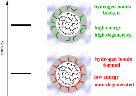
For each chain conformation $m$, the first shell interaction is extensive with respect to $A_{m}$. The links between a solvent node and the chain beads account for the first shell contribution. The non-degenerated ground state denoted by $\beta=0$ models the first shell water molecules with formed hydrogen bonds around the protein. It is taken as the energy reference which equals 0. The excited states, corresponding to $\beta\geq 1$, are for the $g_{\rm sh}^{A_{m}}$ first shell structures with broken hydrogen bonds. Their energy is $A_{m}\ \varepsilon_{\rm sh}$. The Hamiltonian of the first shell solvent for the chain structure $m$ is written :

$${\cal H}^{\rm shell}_{m\beta}=A_{m}\varepsilon_{\rm sh}\sigma(\beta)\ \ \ {\rm with}\ \left\{\begin{array}[]{l}\sigma(0)=0\\ \sigma(\beta)=1\ {\rm if}\ 1\leq\beta\leq g_{\rm sh}^{A_{m}}\end{array}\right.$$

When one intrachain contact is formed, two monomers-solvent bonds are broken. Then, after removing the constant term, the pure solvent contribution is a simple function of $2C_{m}$Collet (2001, 2005). The factor of 2 guarantees that the solvent volume does not depend on the chain structure. For each chain structure $m$, the $g_{\rm bk}^{2C_{m}}$-fold degenerated Hamiltonian of the pure solvent is independent of the bulk micro-state :

$${\cal H}^{\rm bulk}_{m\alpha}=2C_{m}\varepsilon_{\rm bk}\qquad{\rm for}\ 1\leq\alpha\leq g_{\rm bk}^{2C_{m}}$$

The results given in the paper hold while the parameters are ranked as follow : $0<\varepsilon_{\rm bk}<\varepsilon_{\rm sh}$ and $g_{\rm bk}<g_{\rm sh}$. In the spirit of the results obtained by Silverstein et alSilverstein et al. (1999), the values of the solvent parameters are ranked as follow $\varepsilon_{\rm bk}=0.2$, $\varepsilon_{\rm sh}=0.6$, $g_{\rm bk}=2$ and $g_{\rm sh}=3$. The reported results in this paper are quite robust with regards to change the parameters holding the above ranking equation. However, for some technical reasons (discussed below) if $g_{\rm bk}$ or/and $g_{\rm sh}$ are chosen too large, the computational times of the calculation becomes too prohibitive.

The energy and the degeneracy of the ground and excited macro-state of each peptide conformation are :

$$\left.\begin{array}[]{l}{\cal H}^{\rm mac}_{m\sigma}={\cal H}^{\rm ch}_{m}+2C_{m}\varepsilon_{\rm bk}+\sigma A_{m}\varepsilon_{\rm sh}\\ \displaystyle g_{m\sigma}=g_{\rm sh}^{\sigma A_{m}}\ g_{\rm bk}^{2C_{m}}\end{array}\right\}\ {\rm with}\ \sigma=0\ {\rm or}\ 1$$

I.3 Results for the chain in interaction with the solvent

The thermal equilibrium probability of each macro-state is given by : ${\cal P}_{m\sigma}^{\rm eq}=g_{m\sigma}\exp(-{\cal H}^{\rm mac}_{m\sigma}/T)/Z(T)$ and that of a chain structure is $P^{\rm eq}_{m}=\sum_{\sigma=0}^{1}{\cal P}_{m\sigma}^{\rm eq}$. Here the Boltzmann constant is set to 1 and the partition function is:

$$Z(T) = \displaystyle\sum_{m}\sum_{\alpha=1}^{g_{\rm bk}^{2C_{m}}}\sum_{\beta=0}^{g_{\rm sh}^{A_{m}}}\exp\left(-\frac{{\cal H}^{\rm mic}_{m\alpha\beta}}{T}\right)$$ (1)

$$= \displaystyle\sum_{m}g_{\rm bk}^{2C_{m}}\exp\left(-\frac{{\cal H}^{\rm ch}_{m}+{\cal H}^{\rm bulk}_{m\alpha}}{T}\right)$$

$$\displaystyle\left[1+g_{\rm sh}^{A_{m}}\ \exp\left(-\frac{A_{m}\varepsilon_{\rm sh}}{T}\right)\right]$$

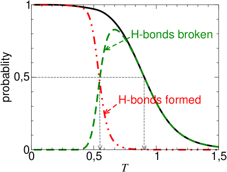
The native conformation is the structure of largest value of $P_{m}^{\rm eq}$ determined by a full enumeration of the conformational space of the chain at low temperature. For the set of couplings $B_{ij}$ and solvent parameters used here, the native conformation is a compact structure of intrachain energy -9.895. The folding transition temperature is defined as, the melting temperature $T_{m}$ of the experimental literaturePrivalov and Privalov (2000); Faisca and Plaxco (2006) at which the equilibrium probability of the native structure equals that of all the other denatured conformations One specific chain structure (the native conformation) has a larger equilibrium probability to occur than all the other conformations for $T<T_{m}$ or in others words $P^{\rm eq}_{\rm Nat}(T_{m})=0.5$ (here $T_{m}=0.90$). Figure 2 shows that the equilibrium probability of occurrence of this native structure (Nat) surrounded by water with formed hydrogen bonds reaches one at low temperature. Other solvent configurations around Nat become relevant for $T>T_{0}$ (here $T_{0}=0.45$). Last, the probability of occurence of the native structure with of the first shell solvent in ES equals that in GS at a specific temperature denoted $T^{*}$ (here $T^{*}=0.54$).

Figure 2: Equilibrium probabilities of occurrence of the native structure (black solid line) as functions of the temperature (given in arbitrary units) with the contribution of the ground state (red long dashed line) and of the excited state (green dashed line). At a temperature $T_{0}$, the probability that the hydrogen bonds are broken becomes significant and at $T^{*}$, the probability to observe hydrogen bonds around the native conformation is the same as that to observe water with broken hydrogen bonds. The probability of occurrence of the native structure equals 1/2 at $T_{m}$.

We note in passing, as the solvent parameter of the GS of the first shell is lower than that of the bulk, it could be possible to observe cold denaturation of the chains, if the GS of the extended chains would be the state of lowest energy among the whole configurational space Collet (2001, 2005). Here, however, the parameterization chosen avoids this possibility in order to study only the folding mechanism.

Figure 3 shows the conformational distribution as function of the number of native intrachain contacts calculated as follow :

$$F_{T}(Q)=-T\ln\sum_{m}\delta(Q-Q_{m})\sum_{\sigma}g_{m\sigma}\exp(-{\cal H}^{\rm mac}_{m\sigma}/T)$$

where $\delta(0=1$ and 0 otherwise and $Q_{m}$ is the number of native contact of the chain structure $m$.

Figure 3: Free energy profile for the lattice model at the three temperatures indicated. $P(Q)$ is the probability of occurrence over $Q$ at thermal equilibrium.

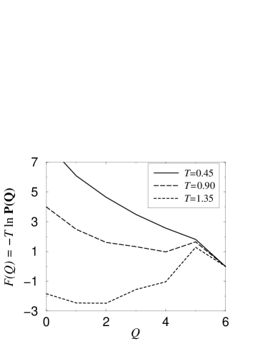
Under denatured conditions ($T>T_{m}$), the free energy profile show a barrier between the native and non-native conditions. The sets of conformation with one or two intrachain contacts, surrounded by solvent in ES (see fig. 4) have the largest probability of occurrence. At the melting temperature, the same barrier still separates the equiprobable native and non-native populations. Under strong native condition (low temperature), the shape of the free energy profile is similar to that observe for a downhill folding.

Indeed, as the temperature decreases, the more probable non-native population shifts from the sets with few native contacts to that with the maximal native contacts

I.4 Results for the solvent at equilibrium

At thermal equilibrium with a bath at temperature $T$, the probability of occurrence of the conformation $m$ with the solvent in micro-state $(\alpha\beta)$ tend towards : $p^{\rm eq}_{m\alpha\beta}=\exp\left(-{{\cal H}^{\rm mic}_{m\alpha\beta}}/{T}\right)/Z(T)$.

The mean energy of the first shell solvent around chain conformation $m$ is :

$$U_{m}^{\rm shell}(T)=\frac{\sum_{\alpha\beta}p^{\rm eq}_{m\alpha\beta}{\cal H}^{\rm shell}_{m\beta}}{\sum_{\alpha\beta}p^{\rm eq}_{m\alpha\beta}}=\frac{A_{m}\varepsilon_{\rm sh}g_{\rm sh}^{A_{m}}\exp(-A_{m}\varepsilon_{\rm sh}/T)}{1+g_{\rm sh}^{A_{m}}\exp(-A_{m}\varepsilon_{\rm sh}/T)}$$

and the heat capacity is :

$$c_{m}^{\rm shell}(T)=\frac{{\rm d}U_{m}^{\rm shell}}{{\rm d}T}=\frac{{A_{m}}^{2}\varepsilon_{\rm sh}^{2}g_{\rm sh}^{A_{m}}\exp(-A_{m}\varepsilon_{\rm sh}/T)}{T^{2}[1+g_{\rm sh}^{A_{m}}\exp(-A_{m}\varepsilon_{\rm sh}/T)]^{2}}$$

These curves as function of the temperature only depends on the chain exposure to the solvent, i.e. on the compactness (fig.4).

Figure 4: The heat capacity of the solvent around the chain structures depends on the compactness of the conformation. At low temperature, the chain are surrounded by rigid cages of water molecules. The higher the compactness, the higher is the temperature of occurrence of the chain with broken hydrogen bonds of the solvent.

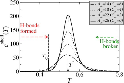
They exhibit a maximum at the same temperature: $T^{*}=0.54$. It is the temperature of equiprobability of occurrence of the two phases: broken and formed hydrogen bonds of the first shell around the peptide. For $T_{0}<T<T^{*}$, the solvent configurations with a water cage around the peptides is preferred to the broken hydrogen bonds. For $T<T_{0}$, it is the only relevant state. Above $T^{*}$, the solvent occurs in the excited macro-state. This is in good agreement with the result obtained for the thermodynamics of the chains presented above.

II Time evolution.

To explore all the possible routes from the non-native structures to the native conformation, the probabilities of each micro-state, composed of one protein structure in interaction with one solvent configuration, evolve using a continuous time Markov process applied to a large sampling of peptides.

Master equation approach to protein folding has already be used in lattice model with an effective solvent Cieplak et al. (1999). It is shown in appendix A, that a master equation of the macro-states may be deduced from the master equation of the micro-states. In a finite time approach, the probabilities of the macro-states evolve following the Euler algorithmCieplak et al. (1998) :

$${\cal P}^{\rm mac}_{m\sigma}(t+\delta t)={\cal P}^{\rm mac}_{m\sigma}(t)+\delta t\sum_{m^{\prime}}\sum_{\sigma^{\prime}}Y_{m\sigma,m^{\prime}\sigma^{\prime}}{\cal P}^{\rm mac}_{m^{\prime}\sigma^{\prime}}(t)$$

where

$$Y_{m\sigma,m^{\prime}\sigma^{\prime}}=g_{m\sigma}\ \frac{V^{(0)}_{mm^{\prime}}}{\tau^{\rm mic}_{m,m^{\prime}}}(1+\exp(({\cal H}^{\rm mac}_{m\sigma}-{\cal H}^{\rm mac}_{m^{\prime}\sigma^{\prime}})/T)^{-1}$$

for $m\neq m^{\prime}$ or $\sigma\neq\sigma^{\prime}$ and

$$Y_{m\sigma,m\sigma}=-\sum_{m^{\prime}\sigma^{\prime}\neq m\sigma}Y_{m^{\prime}\sigma^{\prime},m\sigma}$$

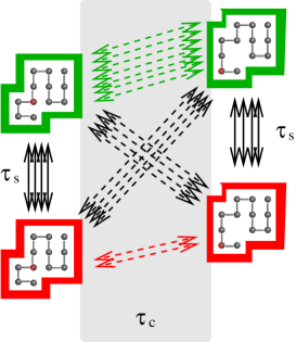
As explained in appendix A, $V^{(0)}_{mm^{\prime}}=1$ if structures $m$ and $m^{\prime}$ are connected by a one monomer move (either a corner flip or a tail move) or if $m=m^{\prime}$. The characteristic time associated to a chain move ($\tau^{\rm mic}_{m,m^{\prime}}=\tau_{c}$ if $m\neq m^{\prime}$) and to a solvent move ($\tau^{\rm mic}_{m,m^{\prime}}=\tau_{s}$ if $m=m^{\prime}$) are set to $\tau_{c}=1$ and $\tau_{s}=0.001\ll\tau_{c}$.

      

Figure 5: Logarithm of the waiting time $t_{p}$ to observe the native structure with a probability equal to $p$ plotted as a function of the inverse of the temperature for $p=0.02$ to $p=0.20$ by steps of 0.02.

A sufficient condition to conserve the norm of the probability vector (i.e. $\sum_{m\sigma}{\cal P}^{\rm mac}_{m\sigma}(t)=1$) is satisfied by fixing $\delta t=1/\max_{m\sigma}\{Y_{m\sigma,m\sigma}\}$. As the values of $g_{m}\sigma$ and then those of $Y_{m\sigma,m^{\prime}\sigma^{\prime}}$ may be huge, the value of $\delta t$ is tiny. Then, the evolution of the probability vector is very slow.

The simulations of folding start with the initial condition : ${\cal P}^{\rm mac}_{m\sigma}(0)=1/2N_{\rm conf}$ where $N_{\rm conf}=15019$ is the number of chain structures. The probability of occurrence of conformation $m$ after time $t$ is $P_{m}(t)={\cal P}^{\rm mac}_{m;0}(t)+{\cal P}^{\rm mac}_{m;1}(t)$. The waiting time to observe the native structure with a probability $p$ is noted $t_{p}$. The main results of the calculation are summarized in fig.5 and 6. They exhibit some findings on the out of equilibrium folding of a large sampling of chains at different temperatures.

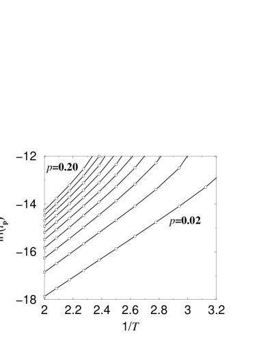
Figure 5 shows a non-Arrhenius behavior of the model. Because of the tiny value of $\delta t$, the early events of the folding are shown, here. The remaining part of this plot will be deduced from the results given below. It will be shown that even if the curves may be well fitted by a Vogel-Fulcher-Tamman function ($t_{p}(T)\propto\exp(-E_{a}/(T-T_{0}))$), which is the signature of an $\alpha$-relaxation with a dynamical temperature $T_{0}=T_{0}(p)$, the remaining part of the curves exhibits a more complex shape which can not be capture by effective solvent models.

      

Figure 6: Evolution of the probabilities of occurrence of native structure (back solid line), the contribution of excited state (green dashed line) and of the ground state (red long dashed line) as functions of the time at different temperatures. For temperature of 0.10 and 0.20, some chains topologically close to the native structure reach it very fast because no activation barrier occurs in their pathway. Then, the probability of the ES decreases monotonically to zero and that of the native structure reach a plateau and the kinetics is frozen. As the number of chain structures of the basin do not depend on the temperature, the plots have very similar shapes and the values of the probabilities are very close to each other showing that a local phenomenon is taking place. For temperature of 0.30 and 0.40, the ES of the native conformation (which have a null equilibrium probability) acts as an attractor, in the early events, and reach very rapidly a maximum of its probability of occurrence, much larger than its equilibrium probability. A fast transition takes place towards the GS of the native structure. Then, a slower dynamic regime guides the other chains towards the native structure. Now, the values of the probabilities depend on the temperatures showing that a global mechanism dominates.

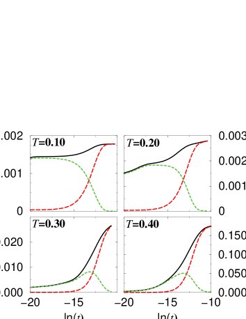
Figure 6 shows that, even if its equilibrium probability is infinitesimal, the excited state of the solvent acts as a strong dynamical attractor above a particular temperature to be discussed later. Below this temperature the kinetics is the same whatever the temperature.

III Relaxation times of the moves.

Only two connected macro-states $(m\sigma)$ and $(m^{\prime}\sigma^{\prime})$ are considered for a while. The equations 6 and 7 show that the rate of the transition $(m^{\prime}\sigma^{\prime})\rightarrow(m\sigma)$ depends on the degeneracy of the macro-state $(m\sigma)$ and not of that of $(m^{\prime}\sigma^{\prime})$. In other words, the increase of the probability of $(m\sigma)$ and the decrease of that of $(m^{\prime}\sigma^{\prime})$ is due to the degeneracy of $(m\sigma)$ and to the difference of energy between the states with $(m^{\prime}\sigma^{\prime})$. After thermal equilibration, the probability of $(m\sigma)$ would go towards ${\cal P}^{(\infty)}_{m\sigma}={{\cal P}^{\rm eq}_{m\sigma}}/({{\cal P}^{\rm eq}_{m\sigma}+{\cal P}^{\rm eq}_{m^{\prime}\sigma^{\prime}}})$ The solution of the system of equations 6, for only two states is :

$${\cal P}^{\rm mic}_{m\sigma}(t)={\cal P}^{(\infty)}_{m\sigma}+[{\cal P}_{m\sigma}(0)-{\cal P}^{(\infty)}_{m\sigma}]\ \exp(-t/\overline{\tau}_{m\sigma,m^{\prime}\sigma^{\prime}})]$$

with a very small relaxation time :

$$\overline{\tau}_{m\sigma,m^{\prime}\sigma^{\prime}}=(Y_{m\sigma,m^{\prime}\sigma^{\prime}}+Y_{m\sigma,m^{\prime}\sigma^{\prime}})^{-1}\ll\tau^{\rm mic}_{m,m^{\prime}}$$ (2)

which now depends on the energies and degeneracies of the macro-states. While numerous chains initially in state $(m\sigma)$ move into state $(m^{\prime}\sigma^{\prime})$, some of them may go back to $(m\sigma)$. As a consequence, the relaxation times depend on forward and backward rates of a move. As an aside, if the move from $(m\sigma)$ to $(m^{\prime}\sigma^{\prime})$ were allowed and not the backward transition, then the relaxation time would simplify to $1/Y_{m\sigma,m^{\prime}\sigma^{\prime}}$.

As the degeneracy of the excited state is always larger than that of the ground state, the value of the rates between two excited states of the chain is larger than that between two ground states (if the energy difference is of the same order) As a consequence, the relaxation times of the former transitions are always very small at not too low temperature. They are supposed to simulate peptide evolving in a fluid solvent. In contrast, the relaxation times of the latter transitions are larger. This models chains evolving in a viscous medium. Thus, the dynamics of the chains surrounded by water with broken hydrogen bonds is faster than that of low degenerated structures in interaction with solvent with formed hydrogen bonds.

In addition, the more extended the structure, the larger the degeneracy of the excited states and the smaller is the relaxation time. This is because a more extended chain has a larger exposure to the solvent and thus a lot of hydrogen bonds are broken in the first shell and as a consequence the dynamics is faster.

Last the connexion between the excited and ground states of the same chain conformation ($m\equiv m^{\prime}$) have a small relaxation time because $\tau_{s}\ll\tau_{c}$. The difference between that case and the fluid connexion depends on the ratio $\tau_{c}/\tau_{s}$.

IV Fast folding mechanism

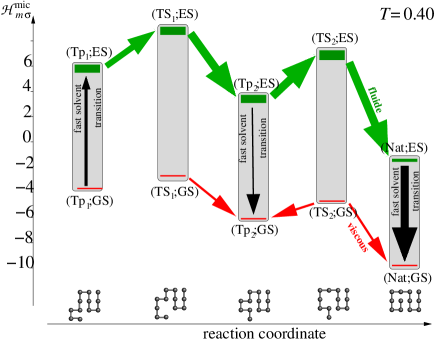
To understand the mechanism underlying the fast folding, a possible pathway leading to the native structure, shown in fig.7, is considered as a first approach of the problem.

Figure 7: Top: A possible pathway with five chain structures connected by one monomer moves ending in Nat taken as an example to capture the role play by the solvent in the folding kinetics. The energy of the GS is given above of each conformation. A single route from Tp₁ to Nat is considered, to simplify the study of this first approach, and the reaction coordinate is simply a function (not given) of the number of conformational changes necessary to reach Nat. Bottom: the waiting times to observe a ratio $p$ of proteins in Nat, starting from an equiprobability of all the states, show a glass transition at temperatures depending on $p$ (shown in the inset).

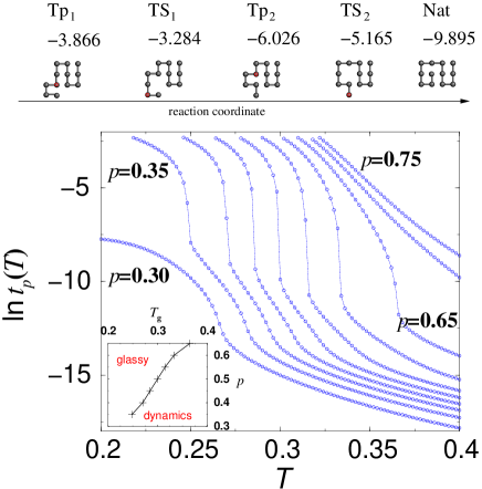
This pathway consists in five chain structures connected by one monomer moves. In contrast with the whole conformational space where there exist a great number of routes from a given conformation to the native structure, in this section we first consider a simplified trajectory where there is a unique pathway (via TS₁, Tp₂ and TS₂) from Tp₁ to Nat. Structures Tp₁ and Tp₂ have five intrachain contacts and thus, smaller energy than TS₁ and TS₂ which have three intrachain contacts. Then, the GS of the structures Tp₁ and Tp₂ should act as kinetics traps and that of TS₁ and TS₂ as transition states towards the native conformation. At $t=0$, the initial probability of each macro-state is set to $P(t=0)=0.1$. An Euler algorithm is applied to simulate the evolution of the probabilities of the ten macro-states of this subsystem composed by the ES and the GS of this five chain structures. The waiting time $t_{p}$ to observe the native structure with a probability equal to $p$ is plotted for $p=0.30$ to $p=0.65$ by steps of 0.05 as function of the temperature. At $t=0$, the probability of occurrence of Nat is already 0.20 and for $p<0.30$, the waiting time is tiny since a many chains in the TS₂ states fold instantaneously in Nat. For $T<0.20$, the waiting time to reach a ratio $p=0.30$ becomes constant, but that to observe a larger ratio become huge.

For $p>0.30$, the waiting times increase continuously as the temperature is decreased until a temperature, depending on $p$ and denoted by $T_{g}(p)$, where a broad dynamical transition occurs. The kinetics is fluid above $T_{g}$ and glassy below.

Figure 8 shows the very early events of the folding of this small system. The ES of Nat relax into the GS via a, very fast, solvent transition. At a temperature independent time, $t_{0}$, the probability of the ES of Nat becomes very small.

Figure 8: . Evolution of the probabilities of the native structure (black solid lines) and the ES (green dashed lines) and the GS (red long dashed lines) contributions as functions of the time for different temperatures.

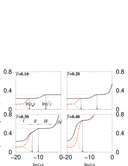
At low temperature ($T=0.10$ or $T=0.20$), half of the chains in conformation TS₂ fold in Nat and the other half goes to Tp₂ between the time $t_{0}$ and a temperature dependent time, $t^{*}$ after which the probability of occurrence of the native structure becomes constant for a while. Then, a long plateau with $p\approx 0.3$ occurs where the dynamics is glassy.

At higher temperature, the probability of occurrence of Nat at $t_{0}$ becomes higher and the length of the plateau smaller. Many chains in the Tp₁, TS₁ or Tp₂ jump to Nat. At $T=0.40$, the probability of the ES becomes very high ($\approx 0.3$) at a time denoted by $t_{M}$ in the early events and the probability of Nat equals 0.8 very fast. Between $t_{M}$ and $t^{*}$, the solvent of the chains in ES relax in GS. Here, the ES of Nat acts as a strong dynamical attractor.

The instantaneous flux from $(m^{\prime}\sigma^{\prime})$ to $(m\sigma)$, given by $k_{m^{\prime}\sigma^{\prime}\rightarrow m\sigma}=Y_{m\sigma,m^{\prime}\sigma^{\prime}}{\cal P}_{m^{\prime}\sigma^{\prime}}(t)-Y_{m^{\prime}\sigma^{\prime},m\sigma}{\cal P}_{m\sigma}(t)$ can also be calculated. Figure 9 shows that, at $T=0.10$, the kinetics is only guided by the difference of energy of the micro-states.

Figure 9: The direction and magnitudes of the flux of the connexion of the pathway shown in fig.7 at $t_{0}$ and $T=0.10$. The larger the flux, the wider is the line. Connections with tiny flux are not drawn.

Figure 10: Same than fig.9 at $T=0.40$. Flux in the GS pathway is the same for both simulations.

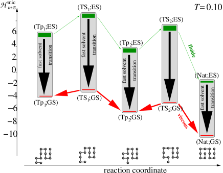
The solvated chains have a very large probability to move towards a micro-state of lower energy. Between the initial time and $t_{0}$, the ES of Nat relax very fast to the GS of Nat. During this period, the ES of all structures relax to the GS. Between the times $t_{0}$ and $t^{*}$, TS₁ and TS₂ relax to Tp₁, Tp₂ and Nat. The probabilities of GS of Tp₁, Tp₂ and Nat increase until all other state have a infinitesimal probability and the probability of the Nat increases to one half of that of TS₂. Then, all the fluxes become tiny and the dynamics is frozen.

At $T=0.40$, the equilibrium probabilities of the ES are infinitesimal. Then, we could also expect a kinetic which would only pass through the ground states, as for $T=0.10$. Instead of this, the sampling of chains finds another strategy to overcome the barrier very fast. At time $t_{0}$, the probability of the GS of Nat is already of 0.6. The flux between the pairs of states, drawn in fig.10, show that the chains in GS of Tp₁ do not fold via the GS of the other structures of the pathway. First, they reach the ES of Tp₁ and then they pass through the ES of the other structures and lastly they relax to the GS of Nat. This is a consequence of the larger transition rates between the ES than between the GS. In addition, the probabilities of the ES remain very small.

The chains follow a pathway with large transition rates between improbable states for which the in going flux equals the out going keeping their probabilities small.

At time $t_{0}$, the probability of Nat is around 0.7. The probabilities of the ES are quasi-null. The flux via the ES pathway is the same as via the GS pathway. The kinetics become very slow and then a plateau occurs in the curves of the probability of Nat as a function of the time shown previously.

V How water lubricates or freezes the folding. A physical picture.

Curves of figs. 6 and 8 are not exactly the same but are similar. The basic mechanisms found for the direct fold in the case of the five-chain conformations pathway may be extended to the whole configurational space of the protein. Put together, the results of this paper allow us to give the picture of the folding given in fig.11.

Figure 11: Top: At $T=0.10$, the chains in any energy level of the ES-funnel relax very fast in the GS-barrel. Then, they move down slowly in the barrel, they reach the trap zone and the dynamics is frozen. Only a tiny fraction of the chains, synthesized in chain structures very close to Nat, reach it in a reasonable time. Bottom: The picture of the folding at higher temperature but below $T_{0}$ where the ES of the chains still has an infinitesimal equilibrium probability, depicts a different mechanism. At $T=0.40$, the chains in the GS-barrel move to the ES-funnel. Then, most of them fold very fast towards the bottom of the ES-funnel (in the ES of the native structure) and they relax in the bottom of the GS barrel (in the GS of the native structure). They get round the trap zone by passing in the ES-funnel where the transition rates are very high. A few chains relax in the GS-barrel during their descent in the ES-funnel and then they have slow dynamics. The temperature where the folding mechanism switches from one scenario to the other one is the glass temperature of the system.

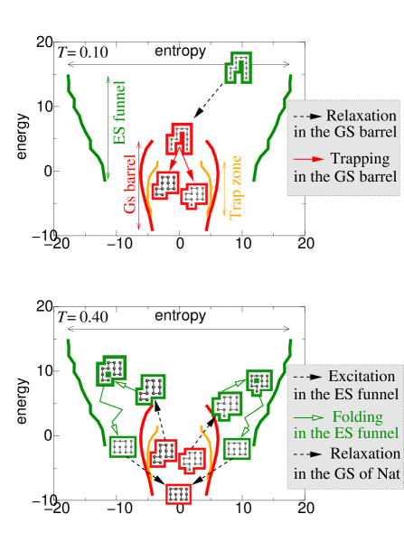
To draw one of the envelop in the energy-entropy plot, the entropy, noted $S_{\sigma}(E)$ for $\sigma=0$, associated to a given microscopic energy, is calculated from the number of chain and solvent configurations, with formed hydrogen bonds. The same calculation, of the entropy noted $S_{\sigma}(E)$ for $\sigma=1$, is done for the solvent without hydrogen bonds. The two functions $S_{\sigma}(E)$ are related to the total number of protein-solvent configurations whose total energy matches the energy values $E$:

$$S_{\sigma}(E)=\ln[\sum_{m}\sum_{\alpha,\beta}\delta(\sigma-\sigma(\beta))\ \ \delta^{(\varepsilon)}(E-{\cal H}^{\rm mic}_{m\alpha\beta})]$$

where $\delta^{(\varepsilon)}(x)=1$ if $-\varepsilon/2<x<\varepsilon/2$ and 0 otherwise. They may be written as functions of the degeneracy of the macro-states:

$$S_{\sigma}(E)=\ln[\sum_{m}g_{m\sigma}\ \delta^{(\varepsilon)}(E-{\cal H}^{\rm mac}_{m\sigma})]$$

Moreover a parameter $\theta_{m}$ allows one to distinguish between the structures of the bottom of the configurational valleys, which may be kinetics traps in the folding. One defines $\theta_{m}=1$ for the macro-states, only connected to macro-states of higher energies and 0 otherwise. Although the native conformation satisfies to this definition, it can not be considered as a trap and the value of $\theta_{\rm Nat}$ is set to 0. Considering the five structures of fig. 7, 9 and 10 as an example, one has $\theta_{\rm Tp_{1}}=\theta_{\rm Tp_{2}}=1$ and $\theta_{\rm TS_{1}}=\theta_{\rm TS_{2}}=\theta_{\rm Nat}=0$. Thus, the envelop of the trap region in the energy-entropy plot is a subset of the GS barrel, given by :

$$S_{\rm{Tp}}(E)=\ln[\sum_{m}\ \theta_{m}g_{m;0}\ \delta^{(\varepsilon)}(E-{\cal H}^{\rm mac}_{m;0})]$$

where $g_{m;0}$ and ${\cal H}^{\rm mac}_{m;0}$ are for the degeneracy and energy of the GS of the structure $m$.

Figure 11 shows the three surfaces drawn on the same plot. The GS-barrel (respectively ES-funnel) is associated to the GS (respectively ES) of the chain structures. A part of the surface of the GS-barrel is populated with the trap conformations We have already shown, in this paper, that the connections between two chain structures in the ES-funnel have small relaxation times and that in the GS-barrel long relaxation times. This results from the following mechanism. A single protein and its solvent is in a given configuration, at a given time, which belongs to a corresponding macro-state, and not in all the configurations of a the macro-state. As a consequence, the transition rates between one protein-solvent configuration of the macro-state $(m\sigma)$ and those of a macro-state $(m^{\prime}\sigma^{\prime})$ depends on the energy difference between these states and also on the degeneracy of $(m^{\prime}\sigma^{\prime})$ but not on the degeneracy of $(m\sigma)$.

In particular, the connexion from a given configuration of the GS to those of the ES of the same chain conformation involves a huge number of routes which increase the energy On the opposite, a few connexions allow the backward transition which decreases the energy.

At ”very low” temperature, the proteins and solvent follow pathways which minimize the microscopic energy. Then, they very slowly evolve, along the few routes of the GS barrel and fall rapidly in some trap conformations.

At ”not too low” temperature, proteins and solvent follow pathways where the number of routes is maximized. Then, they quickly evolve along the vast possibilities of routes of the ES funnel without traps and reach very fast the native structure.

As it has previously been shown, the temperature of glass transition which separates the two mechanisms is not clearly defined because it depends on the ratio of folding proteins

In addition, we mention that, the calculation of the partition function is independent on the informations concerning the network of connexions. As a consequence, the glass temperature is not related to the temperatures ($T_{0}$, $T^{*}$ and $T_{m}$) defined above. This explains why the excited states of the first shell lubricate the folding under conditions where only the ground states have non-nil equilibrium probabilities and why the folding is frozen at lower temperature.

VI Conclusion.

We have shown that a model of protein-solvent which takes into account the difference of degeneracies of the bulk solvent and the first shell solvent with mainly formed or mainly broken hydrogen bonds permits an understanding of the mechanism which may lead to quasi-instantaneous folding of a sufficiently significant ratio of the proteins in solution. Figure 11, shows that two distinct folding mechanisms exist. In the first one, the folding times are very large and in the second one very short.

Appendix A.

The probability of occurrence of the conformation $m$ and the solvent in micro-state $(\alpha,\ \beta)$ at time $t$ is denoted by $p^{\rm mic}_{m\alpha\beta}(t)$. The master equation of the system is written  :

$$\frac{{\rm d}p^{\rm mic}_{m\alpha\beta}}{{\rm d}t}=\sum_{m^{\prime}\alpha^{\prime}\beta^{\prime}}\displaystyle X_{m\alpha\beta;m^{\prime}\alpha^{\prime}\beta^{\prime}}\ p^{\rm mic}_{m^{\prime}\alpha^{\prime}\beta^{\prime}}$$ (3)

where $X_{m\alpha\beta;m^{\prime}\alpha^{\prime}\beta^{\prime}}=X(m^{\prime}\alpha^{\prime}\beta^{\prime}\rightarrow m\alpha\beta)$ is the transition rate from configuration $(m^{\prime}\alpha^{\prime}\beta^{\prime})$ to $(m\alpha\beta)$. The diagonal terms which take into account of the transition from $(m\alpha\beta)$ to the other configurations, are :

$$X_{m\alpha\beta;m\alpha\beta}=-\sum_{(m^{\prime}\alpha^{\prime}\beta^{\prime})\neq(m\alpha\beta)}X_{m^{\prime}\alpha^{\prime}\beta^{\prime};m\alpha\beta}$$

The detailed balance conditions,

$$X_{m\alpha\beta;m^{\prime}\alpha^{\prime}\beta^{\prime}}p^{\rm eq}_{m^{\prime}\alpha^{\prime}\beta^{\prime}}=X_{m^{\prime}\alpha^{\prime}\beta^{\prime};m\alpha\beta}p^{\rm eq}_{m\alpha\beta}$$ (4)

allow to write the rate of transition as :

$$X_{m\alpha\beta;m^{\prime}\alpha^{\prime}\beta^{\prime}}=\frac{V^{(0)}_{mm^{\prime}}}{\tau^{\rm mic}_{m,m^{\prime}}}\ a_{T}({\cal H}^{\rm mic}_{m\alpha\beta};{\cal H}^{\rm mic}_{m^{\prime}\alpha^{\prime}\beta^{\prime}})$$ (5)

where $V^{(0)}_{mm^{\prime}}=V^{(0)}_{m^{\prime}m}=1$ if the two structures are connected by a corner flip and tail movesCollet (2003) (see fig.12)whatever the solvent configurations and $0$ otherwise. The acceptance function is $a_{T}(x;x^{\prime})=[1+\exp((x-x^{\prime})/T)]^{-1}$ and $\tau^{\rm mic}_{m,m^{\prime}}$ is a symmetric function : $\tau^{\rm mic}_{m,m^{\prime}}=\tau_{c}$ if $m\neq m^{\prime}$ and $\tau^{\rm mic}_{m,m^{\prime}}=\tau_{s}$ if $m=m^{\prime}$.

Figure 12: Two types of moves, with different characteristic times, are considered in the dynamics: the protein monomer move (dashed arrows) or the solvent configuration transition (other arrows). For this last event, the connection between solvent configurations of the same macroscopic level do not affect the kinetics. The solvent transition is supposed to have smaller relaxation time than the monomer move. The relaxation times of the connection are defined as follows: we solve eqs.3 and 5 for an isolated connexion between two states $(m\sigma)$ and $(m^{\prime}\sigma^{\prime})$ leading to: $p^{\rm mic}_{m\alpha\beta}(t)=p^{(\infty)}_{m\alpha\beta}+[p_{m\alpha\beta}(0)-p^{(\infty)}_{m\alpha\beta}]\exp(-t/\tau^{\rm mic}_{m,m^{\prime}})$. $\tau^{\rm mic}_{m,m^{\prime}}$ is chosen as $\tau_{c}$ if the connexion is between two different protein structures and is chosen as $\tau_{s}$ if only water moves ($\tau_{s}\ll\tau_{c}$). The set of one monomer moves considered here, is the corner flip (shown in this figure) and the tail move (not shown).

The probability of occurrence of the macro-state $(m\sigma)$ at time $t$ denoted

$${\cal P}^{\rm mac}_{m\sigma}(t)=\sum_{\alpha,\beta}p^{\rm mic}_{m\alpha\beta}(t)\ \delta(\sigma-\sigma(\beta))$$

where $\delta(0)=1$ and $\delta(n)=0$ if $n\neq 0$ and the following relations :

$$\begin{array}[]{ll}\displaystyle\sum_{\alpha^{\prime}\beta^{\prime}}p^{\rm mic}_{m^{\prime}\alpha^{\prime}\beta^{\prime}}&\displaystyle=\sum_{\sigma^{\prime}}\sum_{\alpha^{\prime}\beta^{\prime}}p^{\rm mic}_{m^{\prime}\alpha^{\prime}\beta^{\prime}}\delta(\sigma^{\prime}-\sigma(\beta^{\prime}))\\ &\displaystyle=\sum_{\sigma^{\prime}}{\cal P}^{\rm mac}_{m\sigma^{\prime}}\end{array}$$

$$\sum_{\alpha\beta}\delta(\sigma-\sigma(\beta))=g_{m\sigma}$$

will be used below.

Now, we rewrite the master equation 3 as :

$$\begin{array}[]{l}\displaystyle\sum_{\alpha\beta}\frac{{\rm d}p^{\rm mic}_{m\alpha\beta}}{{\rm d}t}\displaystyle\delta(\sigma-\sigma(\beta))=\\ \displaystyle\sum_{\alpha\beta}\sum_{m^{\prime}\alpha^{\prime}\beta^{\prime}}\delta(\sigma-\sigma(\beta))X_{m\alpha\beta m^{\prime}\alpha^{\prime}\beta^{\prime}}\ p^{\rm mic}_{m^{\prime}\alpha^{\prime}\beta^{\prime}}\end{array}$$

yields :

$$\begin{array}[]{lll}\displaystyle\sum_{\alpha\beta}\frac{{\rm d}p^{\rm mic}_{m\alpha\beta}}{{\rm d}t}&\hskip-8.5359pt\delta(\sigma-\sigma(\beta))=\displaystyle\sum_{m^{\prime}}\sum_{\alpha\beta}\delta(\sigma-\sigma(\beta))\sum_{\sigma^{\prime}}\sum_{\alpha^{\prime}\beta^{\prime}}\ \cdot\\ &\displaystyle\delta(\sigma^{\prime}-\sigma(\beta^{\prime}))\frac{V^{(0)}_{mm^{\prime}}}{\tau^{\rm mic}_{m,m^{\prime}}}a_{T}({\cal H}^{\rm mic}_{m\alpha\beta};{\cal H}^{\rm mic}_{m^{\prime}\alpha^{\prime}\beta^{\prime}})\ p^{\rm mic}_{m^{\prime}\alpha^{\prime}\beta^{\prime}}\end{array}$$

The evolution equation is rewritten :

$$\frac{{\rm d}{\cal P}^{\rm mac}_{m\sigma}(t)}{{\rm d}t}=\sum_{m^{\prime}}\sum_{\sigma^{\prime}}Y_{m\sigma,m^{\prime}\sigma^{\prime}}\ {\cal P}^{\rm mac}_{m^{\prime}\sigma^{\prime}}$$ (6)

with

$$Y_{m\sigma,m^{\prime}\sigma^{\prime}}=g_{m\sigma}\ \frac{V^{(0)}_{mm^{\prime}}}{\tau^{\rm mic}_{m,m^{\prime}}}\ a_{T}({\cal H}^{\rm mac}_{m\sigma};{\cal H}^{\rm mac}_{m^{\prime}\sigma^{\prime}})$$ (7)

In addition, we mention that this result also satisfies the following balance equation: $Y_{m\sigma,m^{\prime}\sigma^{\prime}}{\cal P}^{\rm eq}_{m^{\prime}\sigma^{\prime}}=Y_{m^{\prime}\sigma^{\prime},m\sigma}{\cal P}^{\rm eq}_{m\sigma}$.

References

- Xu et al. (2006) Y. Xu, P. Purkayastha, and F. Gai, J. Am. Chem. Soc. 128, 15836 (2006).
- Sci (2005) Science 309, 86 (2005).
- Levinthal (1968) C. Levinthal, J. Chim. Phys. 65, 44 (1968).
- Dill et al. (2007) K. A. Dill, S. B. Ozkan, T. R. Weikl, J. D. Chodera, and V. A. Voelz, Current Opinion in Structural Biology 17, 342 (2007).
- Kim and Baldwin (1990) P. Kim and R. Baldwin, Ann. Rev. Biochem. 59, 631 (1990).
- Jackson (1998) S. Jackson, Folding Design 3, 81 (1998).
- Kubelka and Hofrichter (2004) J. Kubelka and W. A. Hofrichter, J. andEaton, Curr. Opin. Struct. Biol. 14, 76 (2004).
- Schonbrun and Dill (2003) J. Schonbrun and K. Dill, Proc. Natl. Acad. Sci. USA 100, 12678 (2003).
- Matouschek et al. (1989) A. Matouschek, K. Jr., J.T., L. Serrano, and A. Fersht, Nature 340, 122 (1989).
- Ghosh et al. (2007) K. Ghosh, S. Ozkan, and K. Dill, J.A.C.S. 129, 11920 (2007).
- Zhu et al. (2003) Y. Zhu, D. Alonso, K. Maki, C.-Y. Huang, S. Lahr, V. Daggett, H. Roder, W. Delgado, and F. Gai, Proc. Natl. Acad. Sci. USA 100, 15486 (2003).
- Chan and Dill (1998a) H. Chan and K. Dill, Proteins: Struct. Funct. and Genet. 30, 2 (1998a).
- Akmal and Muñoz (2004) A. Akmal and V. Muñoz, Proteins: Struct. Funct. and Genet. 57, 142 (2004).
- Leopold et al. (1992) P. E. Leopold, M. Montal, and J. N. Onuchic, Proc. Natl. Acad. Sci. USA 89, 8721 (1992).
- Bryngelson et al. (1995) J. D. Bryngelson, J. N. Onuchic, N. D. Socci, and P. G. Wolynes, Proteins Struct. Funct. Genet. 21, 167 (1995).
- Onuchic et al. (1996) J. N. Onuchic, N. D. Socci, Z. Luthey-Schulten, and P. G. Wolynes, Folding & Design 1, 441 (1996).
- Wolynes (1997) P. Wolynes, Proc. Natl. Acad. Sci. 94, 6170 (1997).
- Socci et al. (1998) N. D. Socci, J. N. Onuchic, and P. G. Wolynes, Proteins Struct. Funct. Genet. 32, 1136 (1998).
- Onuchic and G. (2004) J. N. Onuchic and W. P. G., Current Opinion in Structural Biology 14, 70 (2004).
- Clark (2004) P. Clark, Trends in Biochemical Sciences 29, 527 (2004).
- Lau and Dill (1989) K. F. Lau and K. A. Dill, Macromolecules 22, 3986 (1989).
- Gõ (1983) N. Gõ, Annu. Rev. Biophys. Bioeng. 12, 183 (1983).
- Dinner et al. (1994) A. Dinner, A. Šali, M. Karplus, and E. Shakhnovich, J. Chem. Phys. 101, 1444 (1994).
- Collet (2001) O. Collet, Europhys. Letters 53, 93 (2001).
- Chan and Dill (1991) H. S. Chan and K. A. Dill, Annu. Rev. Biophys. Chem. 20, 447 (1991).
- Chan and Dill (1994) H. S. Chan and K. A. Dill, J. Chem. Phys. 100, 9238 (1994).
- Chan and Dill (1998b) H. S. Chan and K. A. Dill, Proteins Struct. Funct. Genet. 30, 2 (1998b).
- Derrida (1981) B. Derrida, Phys. Rev. B 24, 2613 (1981).
- Shakhnovich and Gutin (1990) E. I. Shakhnovich and A. M. Gutin, Nature 346, 773 (1990).
- Šali et al. (1994a) A. Šali, E. Shakhnovich, and M. Karplus, J. Mol. Biol. 235, 1614 (1994a).
- Šali et al. (1994b) A. Šali, E. Shakhnovich, and M. Karplus, Nature 369, 248 (1994b).
- Gutin et al. (1995a) A. M. Gutin, V. I. Abkevich, and E. I. Shakhnovich, Proc. Natl. Acad. Sci. USA 92, 1282 (1995a).
- Gutin et al. (1995b) A. M. Gutin, V. I. Abkevich, and E. I. Shakhnovich, Biochemistry 34, 3066 (1995b).
- Privalov (1990) P. L. Privalov, Crit. Rev. Biochem. Mol. Biol. 25, 281 (1990).
- Nishi et al. (1994) I. Nishi, N. Kataoka, F. Tokunaga, and Y. Goto, Biochemistry 33, 4903 (1994).
- Kumar et al. (2006) R. Kumar, A. Prabhu, D. Rao, and A. Bhuyan, J. Mol. Biol. 364, 483 (2006).
- Kauzmann (1959) W. Kauzmann, Adv. Protein Chem. 14, 1 (1959).
- Warshel and Lifson (1970) A. Warshel and S. Lifson, J. Chem. Phys. 53, 582 (1970).
- Dill (1990) K. Dill, Biochemistry 29, 7133 (1990).
- De Los Rios and Caldarelli (2000) P. De Los Rios and G. Caldarelli, Phys. Rev. E 62, 8449 (2000).
- De Los Rios and Caldarelli (2001) P. De Los Rios and G. Caldarelli, Journal of Biological Physics 27, 229 (2001).
- Collet (2005) O. Collet, Europhys. Letters 72, 301 (2005).
- Chan (2004) H. Chan, La Physique au Canada 60, 195 (2004).
- Garde et al. (1996) S. Garde, G. Hummer, A. E. Garcia, M. E. Paulaitis, and L. R. Pratt, Phys. Rev. Lett. 77, 4966 (1996).
- Hummer et al. (1998) G. Hummer, S. Garde, A. E. Garcia, M. E. Paulaitis, and L. R. Pratt, J. Phys. Chem. B 102, 10469 (1998).
- Garde et al. (1999) S. Garde, A. E. Garcia, L. R. Pratt, and H. Hummer, Biophysical Chemistry 78, 21 (1999).
- Gomez et al. (1999) M. A. Gomez, L. R. Pratt, G. Hummer, and S. Garde, J. Phys. Chem. B 103, 3520 (1999).
- Lyndell-Bell and Rasaiah (1997) R. M. Lyndell-Bell and J. C. Rasaiah, J. Chem. Phys. 107, 1981 (1997).
- Pratt and Chandler (1997) L. Pratt and D. Chandler, J. Chem. Phys. 67, 3683 (1997).
- Shimizu and Chan (2000) S. Shimizu and H. Chan, J. Chem. Phys. 113, 4683 (2000).
- Kaya and Chan (2003) H. Kaya and H. Chan, J. Mol. Biol. 326, 911 (2003).
- Kaya et al. (2005) H. Kaya, Z. Liu, and H. Chan, Biophysical Journal 89, 520 (2005).
- Ferguson et al. (2009) A. Ferguson, Z. Liu, and H. Chan, J. Mol. Biol. 389, 619 (2009).
- Fenimore et al. (2004) P. Fenimore, H. Frauenfelder, B. McMahon, and R. Young, Proc. Natl. Acad. Sci. USA 101, 14408 (2004).
- Frauenfelder et al. (2006) H. Frauenfelder, P. Fenimore, G. Chen, and B. McMahon, Proc., Natl., Acad., Sci., USA 103, 15469 (2006).
- Lubchenko et al. (2005) V. Lubchenko, P. Wolynes, and H. Frauenfelder, J. Phys. Chem. 109, 7488 (2005).
- Shenogina et al. (2008) N. Shenogina, P. Keblinski, and S. Garde, J. Chem. Phys. 129, 155105 (2008).
- Frauenfelder et al. (2009) H. Frauenfelder, G. Chen, J. Berendzen, P. W. Fenimore, H. Jansson, B. H. MacMahon, I. R. Stroe, J. Swenson, and R. D. Young, PNAS 106, 5129 (2009).
- Zanotti et al. (2008) J. M. Zanotti, G. Gibrat, and M. C. Bellisent-Funel, Phys. Chem. Chem. Phys. 10, 4865 (2008).
- Doster et al. (1989) W. Doster, S. Cusack, and W. Petry, Nature 337, 754 (1989).
- Muller (1990) N. Muller, Acc. Chem. Res. 23, 23 (1990).
- Lee and Graziano (1996) B. Lee and G. Graziano, J. Am. Chem. Soc. 118, 5163 (1996).
- Silverstein et al. (1999) K. A. T. Silverstein, A. D. J. Haymet, and K. A. Dill, J. Chem. Phys. 111, 8000 (1999).
- Ben-Naïm (1970) A. Ben-Naïm, J. Chem. Phys. 54, 3682 (1970).
- Becker and Collet (2006) J.-P. Becker and O. Collet, Journal of Molecular Structure. Theochem 774, 23 (2006).
- Chipot et al. (1999) C. Chipot, B. Maigret, and A. Pohorille, Proteins Struct. Funct. Genet 36, 383 (1999).
- Lee and Richards (1971) B. Lee and F. M. Richards, J. Mol. Biol. 55, 379 (1971).
- Eisenberg and McLachlan (1986) D. Eisenberg and A. McLachlan, Nature 319, 199 (1986).
- Wesson and Eisenberg (1992) L. Wesson and D. Eisenberg, Protein Science 1, 227 (1992).
- Ooi et al. (1993) T. Ooi, M. Ootabake, G. Nemethy, and H. Scheraga, P.N.A.S. 84, 3086 (1993).
- Collet and Premilat (1996) O. Collet and S. Premilat, International Journal of Peptide and Protein Research 47, 239 (1996).
- Premilat and Collet (1997) S. Premilat and O. Collet, Europhysics Letters 39, 575 (1997).
- Collet (2008) O. Collet, J. Chem. Phys. 129, 155101 (2008).
- Collet et al. (1997) O. Collet, S. Premilat, B. Maigret, and H. A. Scheraga, Biopolymers 42, 363 (1997).
- Liu and Chan (2005) Z. Liu and H. Chan, Physical Biology 2, S75 (2005).
- Hardin et al. (2002a) C. Hardin, M. P. Eastwood, M. Prentiss, Z. Luthey-Schulten, and P. G. Wolynes, J. Comp. Chem. 23, 138 (2002a).
- Hardin et al. (2002b) C. Hardin, T. V. Pogorelov, and Z. Luthey-Schulten, Current Opinion in Structural Biology 12, 176 (2002b).
- Privalov and Privalov (2000) G. Privalov and P. Privalov, Methods Enzymol. 323, 31 (2000).
- Faisca and Plaxco (2006) P. Faisca and K. Plaxco, Protein Sci. 15, 1608 (2006).
- Cieplak et al. (1999) M. Cieplak, M. Henkel, and J. Banavar, cond-mat/9806313 (1999).
- Cieplak et al. (1998) M. Cieplak, M. Henkel, J. Karbowski, and J. Banavar, Phys. Rev. Lett. 80, 3654 (1998).
- Collet (2003) O. Collet, Phys. Rev. E 67, 061912 (2003).