Computation of Finite Time Lyapunov Exponents using the Perron-Frobenius operator
Abstract
The problem of phase space transport which is of interest both theoretically and from the point of view of applications has been investigated extensively using geometric and probabilistic methods. Two of the important tools for this that emerged in the last decade are the Finite time Lyapunov exponents (FTLE) and the Perron-Frobenius operator. The relationship between these approaches has not been clearly understood so far. In this paper a methodology is presented to compute the FTLE from the Perron-Frobenius operator, thus providing a step towards combining both the methods into a common framework.
Transport on finite time scales in dynamical systems has been studied intensively in the last two decades. A significant motiviation for this study has been transport in fluid systems varying from micro fluidics to geophysical flows. These studies received a significant boost with the development of the concepts of finite time Lyapunov exponents (FTLE) and Lagrangian coherent structures (LCS), [1], [2], [3], which act as transport barriers. A probablistic approach to transport in dynamical systems developed in the last decade, which uses the Perron-Frobenius (PF) operator, [4], to identify the so called almost invariant sets, [5], [6]. The relationship between the two methods has not been well understood though both methods often yield roughly the same results, [7]. In this paper a method to compute the FTLE from the PF operator is given by using an alternative definition of the FTLE based on the covariance of probability density functions. This method of computing the FTLE from the PF operator eliminates the need for long time integrations of trajectories, often a source of errors. The method is illustrated with two simple examples of two dimensional fluid systems. The redefinition of the FTLE along with its computation from the PF operator are a step towards combining the geometric and probabilistic methods into a common framework.
1 Introduction
The problem of phase space transport has important applications such as in mixing and separation problems in fluid flows that vary in scale from the micro to the geophysical, interplanetary transport and instability of mechanical systems, to name a few. A variety of dynamical systems methods have been studied over the past three decades to explain transport mechanisms, to detect barriers to transport, and to quantify transport rates, see eg [1], [2], [3], [5], [6], [8], [9], [10], [11], [12], [13]. These methods fall into two main categories, the geometric and the probabilistic. Under the umbrella of geometric methods are the techniques of invariant manifolds (of fixed points) , lobe dynamics and Finite time Lyapunov exponents (FTLE) and Lagrangian coherent structures (LCS). The method of FTLE and LCS has proven to be particularly useful in studying transport in time dependent systems and has found a variety of applications, for e.g., [14], [15], [16], [17], [18] and [19]. The probabilistic approach studies the transport of densities and the so called almost invariant sets and coherent sets. These methods too have been successfully applied in the study of various geophysical flow problems, [12] and mixing in micro channels [20].
The method of LCS studies stretching and contraction around reference trajectories. The LCS method is therefore local in nature; it provides information about invariant manifolds that determine transport in phase space. The current method of LCS relies on computing the FTLE field using long time computations, since LCS usually can be identified only after a significant time of integration. The disadvantage of this is that, excessive stretching of line elements can introduce computational errors. Moreover specific checks on whether the stretching of line elements is within the linearized regime can be difficult to incorporate in the current algorithms on computing the FTLE. The probabilistic method on the other hand ignores the local transport structures, but using the transfer operator divides the phase space into maximally invariant sets. There have been a few attempts to explore the relationship between the geometric and probabilistic descriptions of phase space transport, such as [7] and [21]. The aim of this short paper is to present a technique of computing the FTLE using the Perron-Frobenius operator that is a step towards combining the geometric and probabilistic methods, by making the Perron-Frobenius operator the common tool to both. By utilizing the Perron-Frobenius operator to compute the FTLE, this method also strengthens the probabilistic interpretation of the FTLE, identified in [21] and [22]. This approach has the added benefits of eliminating the issue of linearization around a reference trajectory in the existing formulation of the FTLE and reduces the time to compute the FTLE field for time-dependent and periodic flows.
2 Review of FTLE and LCS
The formulation of FTLE and the Perron-Frobenius operator is reviewed in this section. This review is intended to provide an intuitive background and set the context for the computation of the FTLE using the Perron-Frobenius operator. For the rigorous definitions and details on these methods, the reader is referred to [5], [6], [2], [3], [1].
2.1 Finite Time Lyapunov exponents
Let be compact and be a smooth flow on . Let the associated vector field be for . Consider a reference trajectory passing through the point and a perturbed trajectory passing through the point at time . The flow maps these points to and at time and the perturbation grows to .
Expanding in a Taylor series about the point we get
| (1) |
The norm or magnitude of can be found using the standard inner product on .
| (2) |
where denotes the transpose and the gradient is evaluated at . The maximum growth of a perturbation is therefore given by the maximum principal stretch, i.e., by the maximum eigenvalue of .
| (3) |
where is the Cauchy-Green tensor. The growth in the perturbation depends on the initial point , initial time and the evolution or integration time .
The leading FTLE gives the time averaged rate of linearized stretching in a neighborhood around a reference trajectory. It is intuitively clear that regions of the phase space with locally high values of FTLE will stretch and separate. The sets with high FTLE act as repelling barriers in the flow. This intuitive idea of barriers is formalized by the concept of Lagrangian coherent structures (LCS), defined as ridges in scalar FTLE field, [2], [3]. Ridges can be defined precisely by appealing to differential geometric quantities as in [23], [2] and [3].
2.2 Perron-Frobenius operator
Let denote the Lebesgue measure and let be a measurable set and be a probability density function, being the space of Lebesgue measurable functions. The unique operator defined by
| (5) |
is called the Perron-Frobenius operator for the flow , [4]. Equation 5 which holds for all measurable sets follows from the Radon-Nykodym theorem.
In practice it is usually necessary to numerically approximate the operator . This is done by discretizing the domain, , into a finite number of sets, say which is essentially a grid of boxes. A projection defined by , where is the characteristic function of the set and gives a finite dimensional approximation of . Since is a probability density function . Similarly is projected on . The operator is a linear operator between finite dimensional vector spaces. Further taking the box measures for all , becomes a stochastic transition matrix. The entries of the matrix are determined by a Monte-Carlo simulation [5] and [6]. Each box in the domain contains a fixed number of points (initial conditions), which are integrated from a time to . The final position of the points gives the matrix as -
| (6) |
A time reversible operator is required to apply the above definition for flows in forward time, [6]. This is achieved by creating a reversible Markov operator given by
| (7) |
where is the time reversed analogue of . Its elements are given by
| (8) |
where and are components of the first left eigenvector, , of . For a volume preserving flow in which the domain is uniformly discretized, , the transpose of . Henceforth for convenience the time reversible operator is referred to simply as unless there is an ambiguity about the initial and final times and . The Markov operator has the semigroup property of , where . This property is used to simplify the computations of the FTLE.
3 Computation of FTLE using the Perron-Frobenius operator
3.1 Definition of set oriented FTLE
The concepts of FTLE and LCS reviewed previously have been used fruitfully in many areas as has been pointed out earlier. However the standard computational implementation of FTLE, using finite differences, suffers from some drawbacks, stemming from the integration time and the linearization around reference trajectories. In equation 1, it is assumed that the second (and higher ) order terms are negligible. However the magnitude of the higher order terms depends on the evolution time . If the evolution time is too high then the higher order terms may be comparable to the first order terms in equation 1. If the evolution time is too low, then one cannot detect any interesting structure in the FTLE field. Often, the evolution time is selected in a subjective fashion without checking the validity of equation 1. The problem with this is illustrated with the example of the double gyre flow, a prototype in the LCS literature, [2, 7]. The double gyre flow is defined by the stream function , with , where we use the parameters , and . The time period of the flow is . Now consider the equation 1 with the second order terms explicitly written,
| (9) |
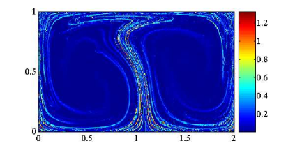
In this equation it can be shown that the second and first order terms are comparable in magnitude. The max-norm for matrices is used for this comparison. Figure 1 shows the plot of and . The magnitude of the second order terms is more than half that of the first order terms in equation 9. This is true for a smaller evolution time as well. The ridges in FTLE field for the double gyre flow are generated by moving instantaneous stagnations points (ISPs) . Material line elements close to the ISPs stretch in a shorter time as compared to material line elements farther away. Therefore ineresting structures such as ridges in the FTLE field require a long period of integration during which the nonlinear deformation of line elements close to the ISPs occurs.
 |
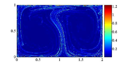 |
| (a) Magnitude of first-order terms in eq. (9) | (b) Magnitude of second-order terms in eq. (9) |
To study the linearized flow in equation 9, numerics have to be carefully planned to ensure that the approximation of linearization is valid. Usually this is accomplished by selecting a very small and either by keeping the time of integration small enough or rescaling the perturbation as it grows very large. If perturbations around a specific trajectory grow too large and need to rescaled, then additional reference points have to be introduced in that region to obtain the FTLE field at a fine enough resolution. Alternatively the computations could start with a crude mesh of initial points and refined iteratively by introducing new initial points based on the finite time stretching, requiring adaptive meshing of initial conditions, which was explored in [17]. However such techniques of mesh refinement are not based on the magnitude of the second order terms in equation 9. Beyond the fact that numerical algorithms for the calculation of FTLE do not check the validity of the linearization of the flow, there is the additional fact that interesting structures in the FTLE field develop for longer eveolution times during which material lines stretch nonlinearly and even fold as shown in figure 2 which was discussed earlier in [17].
The difficulties in the computation of the FTLE can be overcome with a set oriented definition of the FTLE. Instead of tracking only a reference trajectory and the adjacent nodes of the finite difference mesh, one tracks the movement of the whole set (shown in gray) in figure 2 and consider the distribution of points in the set, then folding and nonlinear deformation can be accounted for. A new definition of the FTLE was proposed in [21] which computed the deformation of sets instead of the stretching of line elements and partially addressed the concerns of second order terms, integration time and folding of material lines. We review the new definition here.
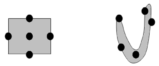
For illustrating the concept we assume the flow is is two dimensional with . The method of computing FTLE using the SVD of the Cauchy-Green tensor essentially computes the linearized stretching of a neighborhood, a set , under the action of the flow as shown in figure 3. The FTLE for the reference trajectory in this case is where is the time of evolution of the trajectory.

In the standard FTLE method the evolution of the set is assumed to be determined by the evolution of two vectors, the directions of principal stretches. For the set oriented definition the deformation of the set is tracked by the evolution of a random vector defined by a probability density function which is initially a uniform probability density function supported on given by, , where is characteristic function of . The covariance matrix of is , with and where is the mean value of the random vector and denotes the expectation with . Under the action of the flow , is mapped to where is the associated Perron-Frobenius operator. In matrix notation the covariance is
| (12) |
Definition 3.1
Let be the covariance of and the covariance of and let denote the maximum eigenvalue of . Then the FTLE of denoted by is defined as -
| (13) |
It can be shown that by direct calculation that the covariance FTLE obtained from Definition 3.1 and the standard FTLE have the same value if the second and higher order terms in equation (9) are negligible when compared to the first order terms. In this case an initial circular blob deforms into an ellipse as shown in figure 3. The eigenvalues of the are and . The standard FTLE is . The covariance matrix for the deformed ellipse is
| (16) |
giving . The covariance matrix is a diagonal matrix with giving . This gives the covariance FTLE, . For volume preserving flows, . This gives the covariance FTLE, , the same value as the standard FTLE. The standard FTLE is obtained by the stretching of the value of the covariance based FTLE is the same as that obtained from traditional FTLE calculation using line stretching.
Since is the covariance of , it provides a probabilistic interpretation of the FTLE. Simultaneously can also be interpreted as the moment of inertia of the set and provides a geometric description of the deformation or distortion of the set. The definition of avoids the linearization of the flow and the computation of the stretching of line elements. Further it is a set-oriented method and directly computes the deformation of a set instead of inferring it from the deformation of line elements. If the linearized flow is valid the covariance FTLE and the standard FTLE are equal. However the covariance FTLE is a better measure of finite deformation of sets. The covariance based method of FTLE is a bridge between the geometric approach of measuring line stretching and the probabilistic approach of almost invariant sets.
In practice any set and a density function supported on has to be approximated by discrete points. If the function is a uniform density function, then can be approximated by points, with coordinates , ranging from 1 to . Each of these points has discrete measure . Similarly is also approximated by the images of the points, , each with measure . For volume preserving flows this is the same as . The covariance for the function , , is approximated by
| (19) |
where is the mean or expected value of the discrete approximation of . The initial covariance matrix can also be obtained similarly. The maximum eigenvalues of and can be plugged into equation (3.1) to give the covariance FTLE.
3.2 Computation of covariance FTLE using Perron-Frobenius operator
The covariance FTLE is a set oriented redefinition of the FTLE. Therefore is natural to expect the Perron-Frobenius operator play a role in the computation of the covariance FTLE. This will be particularly useful since only short time integrations are necessary to calculate the Perron-Frobenius operator . The operator can be found using a suitable set of short time intervals, ; . Let be a uniform density function supported on a set . Then as before maps under the action of the flow to , . For time independent flows or periodic flows with period , this becomes particularly easy, with where for . This avoids long time integration of trajectories.
For two dimensional flows, , the operator is numerically approximated by using the box discretization method described in section 2.2. Each box contains a fixed number of uniformly distributed points. The entries of the matrix are calculated or a suitably chosen and the time reversible operator is found from equations (6), (7) and (8). To compute the FTLE over the entire domain, we take the projection of a uniform density function such that , with the column being equal to the inverse of the measure of . The vector evolves to at , given by,
| (20) |
Similarly the evolution of at time is given by
| (21) |
Equation 21 defines how a set of points uniformly distributed over the set at is disperese at time . The the covariance of this set can be found from the row of as follows
| (24) |
where are the centers (mean values) of each of the boxes, and .
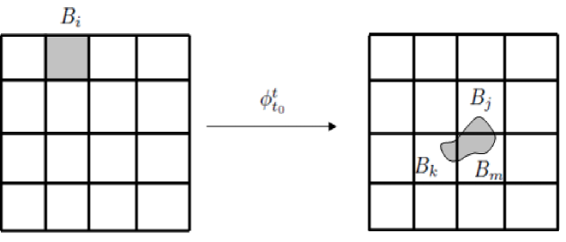
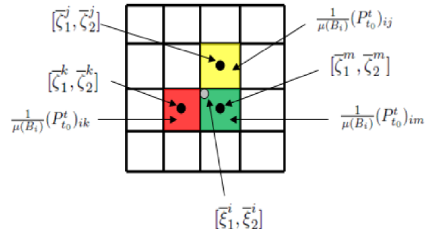
Intuitively the uniformly distributed points in box are mapped into some of the boxes by the flow map , say boxes , and as shown in figure 4. If the number of points that are mapped into each of the three boxes are , and , then each of the three sets , and are approximated by , and uniformly distributed points in the boxes , and . The mean or average of these dispersed points is . The vector with the nonzero values in columns , and . The mean or center of this set is given by . Proceeding thus, the covariance FTLE for each of the boxes in the domain can be found from equation (24).
It should be emphasized that the computation of the FTLE using the Perron-Frobenius operator requires a set oriented definition of the FTLE. One cannot use the operator to track the evolution of sets of zero measure, since the integral on the right hand side of equation 5 is zero for this case. The standard method of FTLE which requires the evolution of individual trajectories passing through the nodal points of a mesh at the initial instant of time, does not make any direct reference to sets of positive measure around these nodal points. Hence a set oriented definition of FTLE is necessary to take advantage of the Perron-Frobenius operator. In practice the computational approach for this new definition too has to make use of discrete initial conditions and trajectories , but sets of positive measure are explicitly modeled by these discrete initial conditions.
4 Examples
In this section we illustrate the computation of the FTLE using the Perron-Frobenius operator for two flows. The first is the lid-driven cavity flow studied for its mixing properties in [20] and the double gyre flow that has been a prototype flow in the LCS and almost invariant sets literature, [2], [17], [7].
4.1 Lid driven cavity flow
The problem of transport in the model of the lid driven cavity flow has been investigated in [20] and is considered here as the first example because of its simple piecewise steady velocity field. The flow is described by the stream function
| (25) |
defined on the domain for time . where
and
For time , the sign of the velocity term is changed. This reflects the streamlines about after a time .
Using symmetry arguments given in [24] and [25], a specific ratio of the magnitudes of the terms along with a fixed value of the period of the flow is found such that it generates three period-3 fixed points in the domain . The specific values of the constants that we borrowed from [24] and [25] are and and for the domain .
A perturbation of the time period of the flow from the critical value of destroys the fixed points. The method of almost invariant sets was used in [26] and [20] to study mixing for different values of the perturbed time period. Since our main interest here is to illustrate the FTLE computed from the Perron-Frobenius operator, we choose a single case, a specific value of half time period for our study.
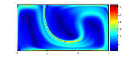
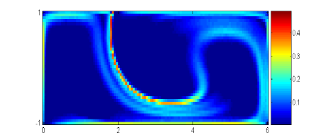
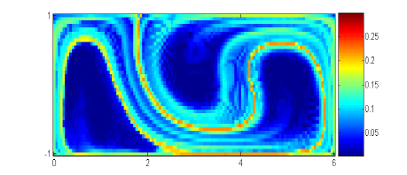
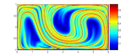
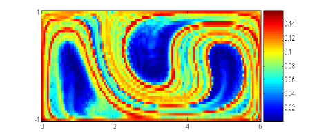
The standard FTLE computation was done for the system for different integration times; , and , the results of which are shown in figure 6(a)-(c) by integrating points initially spaced at a distance of . The domain is then divided into 4800 boxes each box containing a 100 points and the time reversible Perron-Frobenius matrix is found by integrating a total of 480,000 initial points for a period equal to . The vector space has dimensions which are the discretized finite approximation of the infinite dimensional space of Lebesgue integrable functions. Uniform density functions each supported on a box are the bases vectors for the finite dimensional vector space. The covariance based FTLE computation was performed using the Perron-Frobenius operator . Figure 6 (d) is obtained by computing the covariance of the bases functions from the rows , while figure 6 (e) and (f) are obtained by computing the covariance of the basis functions from the rows of and respectively.
 |
 |
| (a) | (d) |
 |
 |
| (b) | (e) |
 |
 |
| (c) | (f) |
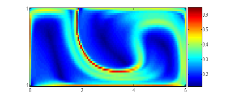
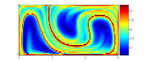
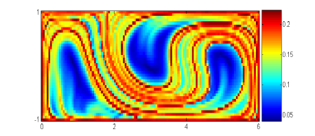
It is evident from the figure 6 that the FTLE field has the same ridge structure when computed by the line stretching approach or the covariance approach using the Perron-Frobenius operator. Computing the covariance based FTLE field directly by integrating all the initial conditions to , while more accurate is computationally more intensive. In fact the time taken for this method increases almost linearly with the integration time. The FTLE field computed from the Perron-Frobenius operator has the same features as the covariance FTLE field by integrating the points in each of the boxes for and computing the covariance of the bases functions which is shown in figure 7.
 |
 |
| (a) | (b) |
(c)
While the FTLE field computed directly by integration and that computed by the Perron-Frobenius operator have the same ridge features, they differ in the magnitude of the FTLE field. This discrepancy in the magnitude is due to two reasons. The Ulam method of approximating the Perron-Frobenius operator by a matrix introduces approximations.The measure of each of the boxes is approximated by a finite number of discrete points introducing further errors. Lastly the calculation of the covariance matrix using equation as explained in figure 4 introduces another level of approximation. As the box size in the computation is reduced and/or the number of points per box is increased, it is natural to expect that the matrix approximation of and the covariance computation become more accurate, though no rigorous proof is offered here.
4.2 Double gyre flow
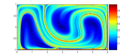
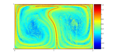
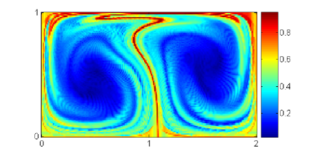
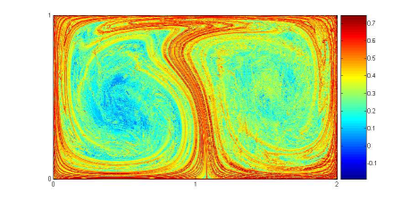
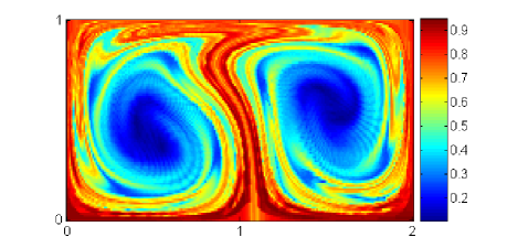
The double gyre flow which is time dependent but periodic, has been one of the prototype flows in the LCS literature, [2], [7]. The double gyre flow is defined by the stream function , with the parameters , and . The time period of the flow is . The domain is discretized into 50000 square boxes of size each containing 625 points. The FTLE field computed using the stretching of line elements and the FTLE field computed from the Perron-Frobenius operator is shown in figure 8.
 |
 |
| (a) | (b) |
 |
 |
| (c) | (d) |
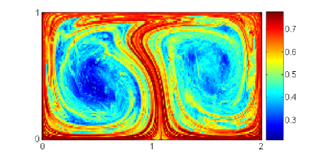
As observed in the discussion on the lid driven cavity flow, the FTLE field has the same ridge features, when the covariance of the sets are computed directly by integrating all the points in each box to , as shown in figure 9 and when computed using the Perron-Frobenius operator. Moreover because of the more accurate approximation of the domain by a higher number of boxes, the covariance FTLE field computed by a direct integration and that computed by the Perron-Frobenius operator are closer to each other in magnitude.
5 Conclusion and Discussion
A method to compute the FTLE field using the Perron Frobenius operator has been introduced in this paper. To do this a modified definition of the FTLE was used which identifies deformation of sets of positive measure instead of the stretching of line elements. This methodology is general enough to be used in time-dependent flows and is particularly useful in the case of time-independent and periodic flows, where it offers a significant computational advantage by eliminating long time integrations. The method of computing the covariance FTLE from Perron-Frobenius operator using equation (24) was illustrated by two examples; the lid driven cavity flow and the double gyre flow. In both cases it was shown that the FTLE field computed by the new method has the same topological features as the FTLE field computed using the standard approach of line stretching and the direct computation of the covariance FTLE from the dispersion of points as in equation (19). The computational time required for the calculation of the covariance FTLE directly from the dispersion of points scales linearly with time in the most ideal case. So the time taken to calculate , for an integration time , is times that of the time taken for calculating . Using the PF operator approach the time necessary to calculate the FTLE is almost independent of the multiple . Thus the method proposed in this paper is times computationally efficient.
Comparing the method proposed in the paper, with that of the standard FTLE, the computation of the standard FTLE is faster. This is because the standard FTLE computations were done a very coarse grid in both the examples presented. Even though the time of integration is shortes, fewer initial conditions have to be integrated and thus the method is faster. However as has been pointed in the paper in section 3.1 this is achieved at the cost of erroneously ignoring the higher order terms in equation (1). The covariance based method of computing the FTLE does not use the linearized equations of a flow making it more general in scope of application.
Moreover the covariance FTLE gives the deformation of sets a probabilistic interpretation. The new method of computing the covariance FTLE introduced in this paper is based on the Perron-Frobenius operator; a common tool in probabilistic methods of phase space transport. This puts the Perron-Frobenius operator at the center of study of phase space transport. This is perhaps intuitively obvious since the Perron-Frobenius operator contains all the information of global transport of sets. The method of computing the covariance FTLE using the Perron-Frobenius operator is a step towards combining the probabilistic and geometric methods of phase space transport, into a common unified framework.
References
- [1] G. Haller. Lagrangian coherent structures and the rate of strain in a partition of two-dimensional turbulence. Physics of Fluids A, 13:3368–3385, 2001.
- [2] S. C. Shadden, F. Lekien, and J. Marsden. Definition and properties of lagrangian coherent structures from finite-time lyapunov exponents in two-dimensional aperiodic flows. Physica D, 212:271–304, 2005.
- [3] F. Lekien, S. C. Shadden, and J. Marsden. Lagrangian coherent structures in n-dimensional systems. Journal of Mathematical Physics, 48, 2007.
- [4] A. Lasota and M. C. Mackey. Chaos, Fractals and Noise. Stochastic Aspects of Dynamics. Springer-Verlag, second edition, 1994.
- [5] M. Dellnitz and O. Junge. On the approximation of complicated dynamical behavior. SIAM Journal on Numerical Analysis, 36:491–515, 1998.
- [6] G. Froyland and M. Dellnitz. Detecting and locating near optimal almost invariant sets and cycles. SIAM Journal on Scientific Computing, 24:1507–1523, 2003.
- [7] G. Froyland and K. Padberg. Almost-invariant sets and invariant manifolds - connecting probabilistic and geometric descriptions of coherent structures in flows. Physica D, 236 (16):1839–1863, 2009.
- [8] S. Wiggins. Chaotic transport in dynamical systems, Interdisciplinary Applied Mathematics. Springer, first edition, 1993.
- [9] K. Ide, D. Small, and S. Wiggins. Distinguished hyperbolic trajectories in time dependent fluid flows: Analytical and computational approach for velocity fields as data sets. Nonlinear Processes in Geophysics, 9:237–263, 2002.
- [10] S. Wiggins. The dynamical systems approach to lagrangian transport in oceanic flows. Annual Review of Fluid Mechanics, 37:295 – 328, 2005.
- [11] G. Froyland, S. Lloyd, and N. Santitissadeekorn. Coherent sets for nonautonomous dynamical systems. Physica D, 239:1527–1541, 2010.
- [12] G. Froyland, N. Santitissadeekorn, and A. Monahan. Transport in time-dependent dynamical systems : Finite time coherent sets. Chaos, 20:043116, 2010.
- [13] P. C. Du Toit. Transport and separatrices in time dependent flows. PhD thesis, California Institute of Technology, 2010.
- [14] C. Coulliette, F. Lekien, J. D. Paduan, G. Haller, and J. Marsden. Optimal pollution mitigation in monterey bay based on coastal radar data and nonlinear dynamics. Environmental Science and Technology, 41:6562–6572, 2007.
- [15] P. Tallapragada and S. D. Ross. Particle segregation by stokes number for small neutrally buoyant spheres in a fluid. Physical Review E, 78, 2008.
- [16] G. Haller and T. Sapsis. Instabilities in the dynamics of neutrally buoyant particles. Physics of fluids, 20, 2008.
- [17] F. Lekien and S. D. Ross. The computation of finite-time lyapunov exponents on unstructured meshes and for non-euclidean manifolds. Chaos: An Interdisciplinary Journal of Nonlinear Science, 2, 20‘0.
- [18] W. Tang, M. Mathur, G. Haller, D. C. Hahn, and F. H. Ruggiero. Lagrangian coherent structures near a subtropical jet stream. Journal Atmospheric Science, 67:2307–2319, 2010.
- [19] M. Wilson, J. Peng, J. O. Dabiri, and J. D. Eldredge. Lagrangian coherent structures in low reynolds number swimming. Journal of Physics: Condensed Matter, 21:204105, 2009.
- [20] M. Stremler, S. Ross, P. Grover, and P. Kumar. Almost invariant sets as ghost rods for fluid stirring. Physical Review Letters, 106, 114101, 2011.
- [21] P. Tallapragada and S. D. Ross. A geometric and probabilistic description of coherent sets. Preprint, Submitted to SIAM Journal of Dynamical Systems, 2011.
- [22] P. Tallapragada. Identifying dynamical boundaries and phase space transport using Lagrangian coherent structures. PhD thesis, Virginia Polytechnic Institute and State University, 2010.
- [23] D. Eeberly. Ridges in Image and Data Analysis. Kluwer Academic Publishers, second edition edition, 1996.
- [24] M. A. Stremler and J. Chen. Generating topological chaos in lid-driven cavity flow. Physics of Fluids, 19:103602, 2007.
- [25] J. Chen and M. A. Stremler. Topological chaos and mixing in a three-dimensional channel flow. Physics of Fluids, 21:021701, 2009.
- [26] P. Grover. Finding and exploiting structure in complex systems via geometric and statistical methods. PhD thesis, Virginia Polytechnic Institute and State University, 2010.