A Partitioning Deletion/Substitution/Addition Algorithm for Creating Survival Risk Groups

Abstract

Accurately assessing a patient’s risk of a given event is essential in making informed treatment decisions. One approach is to stratify patients into two or more distinct risk groups with respect to a specific outcome using both clinical and demographic variables. Outcomes may be categorical or continuous in nature; important examples in cancer studies might include level of toxicity or time to recurrence. Recursive partitioning methods are ideal for building such risk groups. Two such methods are Classification and Regression Trees (CART) and a more recent competitor known as the partitioning Deletion/Substitution/Addition (partDSA) algorithm, both which also utilize loss functions (e.g. squared error for a continuous outcome) as the basis for building, selecting and assessing predictors but differ in the manner by which regression trees are constructed.

Recently, we have shown that partDSA often outperforms CART in so-called “full data” (e.g., uncensored) settings. However, when confronted with censored outcome data, the loss functions used by both procedures must be modified. There have been several attempts to adapt CART for right-censored data. This article describes two such extensions for partDSA that make use of observed data (i.e. possibly censored) loss functions. These observed data loss functions, constructed using inverse probability of censoring weights, are consistent estimates of their uncensored counterparts provided that the corresponding censoring model is correctly specified. The relative performance of these new methods is evaluated via simulation studies and illustrated through an analysis of clinical trial data on brain cancer patients. The implementation of partDSA for uncensored and right censored outcomes is publicly available in the R package, partDSA.

1 Introduction

Clinicians carefully weigh a patient’s prognosis when deciding on the aggressiveness of treatment. In determining a patient’s prognosis, clinicians may consider a patient’s age, gender, clinical information and, more recently, biological variables such as gene or protein expression. Objective guidelines for predicting a patient’s prognosis (i.e., risk) from clinical and biological information can be obtained from risk indices estimated from data collected on an independent sample of patients with known covariates and outcome. Frequently, the outcome of interest is the time to occurrence of a specified event; common examples in cancer include death and recurrence or progression of disease. The use of time-to-event outcomes frequently results in the presence of right-censored outcome data on several patients.

There are many statistical learning methods that might be used in building predictors of risk for a given outcome using covariate information. An attractive class of methods for building clinically interpretable risk indices is recursive partitioning methods. The Classification and Regression Tree algorithm (CART; Breiman et al., 1984) is perhaps the most well-known recursive partitioning method. Left unchecked, CART has the capability of placing each subject in his own terminal node. An important consideration therefore lies in the selection of an appropriate number of splits (i.e., nodes). This “pruning” problem involves an inherent but familiar trade-off: construct an accurate estimator that also avoids overfitting the model to the data. CART uses cross-validation in combination with a specified loss function in order to determine where to stop partitioning the covariate space. In the resulting pruned tree, a single predicted value is assigned to each terminal node. For example, with a continuous outcome and an $L_{2}$ (i.e., squared-error) loss function, the predicted value for each terminal node is the mean outcome for all observations falling into that node.

Molinaro et al. (2010) recently developed partDSA, a new loss-based recursive partitioning method. Like CART, partDSA divides the covariate space into mutually exclusive and disjoint regions on the basis of a chosen loss function. The resulting regression models continue to take the form of a decision tree; hence, partDSA also provides an excellent foundation for developing a clinician-friendly tool for accurate risk prediction and stratification. However, this algorithm differs from CART in that the decision tree may be constructed from both ‘and’ and ‘or’ conjunctions of predictors. The advantage of this representation is two-fold: (i) in cases where only ’and’ conjunctions of predictors are required to build a parsimonious model, the partDSA and CART representations coincide; and, (ii) in cases where CART requires two or more terminal nodes to represent distinct subpopulations (i.e., defined by covariates) having the same outcome distribution, partDSA can represent these same structures using a single partition. Molinaro et al. (2010) showed that this increased flexibility improves prediction accuracy and predictor stability for uncensored continuous outcomes using a $L_{2}$ loss function in comparison to the best adaptive algorithms in the statistical literature, including CART and Logic Regression (Ruczinski et al., 2003).

In both CART and partDSA, the choice of loss function plays a key role in each step of the model building process. The default choice for continuous outcomes (i.e., $L_{2}$ loss) requires modification if these outcomes are censored. Numerous adaptations of CART have been suggested in the literature for handling right-censored outcomes; see, for example, Gordon and Olshen (1985), Ciampi et al. (1986), Segal (1988) Therneau et al. (1990), LeBlanc and Crowley (1992), and LeBlanc and Crowley (1993). With one exception, each of the aforementioned adaptations of CART replaces the usual $L_{2}$ loss function with a criterion function that relies on more traditional estimators and measures of fit used with right censored outcome data. In the absence of censoring, such adaptations typically yield answers that differ from those provided by the default implementation of CART. Adaptations that replace the $L_{2}$ loss function with other criteria also do not allow one to easily quantify the prediction error of the final model using the same loss function. Molinaro et al. (2004) proposed $CART_{IPCW}$, a direct adaptation of CART that replaces the $L_{2}$ loss function with an Inverse Probability Censoring Weighted estimator (IPCW; Robins and Rotnitzky, 1992) of the desired “full data” $L_{2}$ loss function (i.e., that which would be used in the absence of censoring). This allows for an otherwise unaltered implementation of CART to be used for splitting, pruning, and estimation. The IPCW-$L_{2}$ loss function, computable for observed data, is under standard assumptions a consistent estimator of the full data $L_{2}$ loss function. Molinaro et al. (2004) demonstrate that $CART_{IPCW}$ generally has lower prediction error, measured as $L_{1}$ loss using the Kaplan Meier median as the predicted value within a given node, when compared to the one-step deviance method of LeBlanc and Crowley (1992).

In this paper, we similarly extend partDSA to the setting of right-censored data using a IPCW-$L_{2}$ loss function. The resulting methodology builds a decision tree based on the (time-restricted) mean response in each node. We also extend partDSA to the problem of predicting a binary outcome of the form $Z(t)=I(T\geq t),$ where $T$ is the event time of interest and $t$ is some specified time point. This extension involves a weighted modification of the $L_{2}$ loss function that uses the Brier Score (Graf et al., 1999). Graf et al. (1999) introduces this measure as a way to compare the predictive accuracy of various estimators of survival experience. Two novel contributions of this paper are to (i) demonstrate that this score has a simple but interesting representation as an IPCW-weighted $L_{2}$ function; and, (ii) make use of this loss function as the basis for constructing a partDSA regression tree.

The remainder of this paper proceeds as follows. First, we describe the relevant “full data” and “observed data” structures, giving a brief overview of loss-based estimation in each setting. We then discuss how these ideas may be used to extend the partDSA algorithm to right-censored outcomes. The performance of these extensions of partDSA are evaluated via simulations and in an analysis of clinical trial data on brain cancer patients. Finally, we close the paper with a discussion and comments on further, useful extensions.

2 Methods

2.1 Relevant Data Structures

2.1.1 Full Data

In the ideal setting, one observes $n$ i.i.d. observations $X_{1},\ldots,X_{n}$, of a “full data” structure, say $X=(T,W)$, where $T$ denotes a response variable and $W\in\mathcal{S}$ denotes a (possibly high-dimensional) vector of covariates. Denote the corresponding (unknown) distribution of $X$ by $F_{X,0}$. With time-to-event data, our focus hereafter, $T>0$ is a continuous random variable that denotes the event time of interest and $W$ represents a set of baseline covariates. In this case, we may equivalently define the full data as $X=(Z,W)$, where $Z=\log T$. In the setting of cancer risk prediction, $W$ may include age as well as various genomic, epidemiologic and histologic measurements that are continuous or categorical in nature. More generally, the available information may include both time-dependent and time-independent covariates; we focus on the setting of time-independent $W$ only.

2.1.2 Observed Data

In practice, information may be missing on one or more of the $X_{i}s$; that is, one instead observes $n$ i.i.d. observations $O_{1},\ldots,O_{n}$ of an observed data structure $O$ having distribution $F_{Obs}$. With time-to-event outcomes, the most common form of missing data is right-censoring of event times due to drop out or end of follow-up. Here, $O=\{\widetilde{T}=\min(T,C),\Delta=I(T\leq C),W\},$ where $\widetilde{T}=\min(T,C)$ and $\Delta=I(T\leq C)$; equivalently, $O=(\widetilde{Z},\Delta,X)$, where $\widetilde{Z}=\log\widetilde{T}$. The distribution $F_{Obs}$ of $O$ then depends on $F_{X,0}$ and the conditional distribution of the censoring variable $C$ given $X$, say $G_{0}(\cdot|X)$.

We assume that the censoring variable $C$ is conditionally independent of $T$ given $W$; that is, $\bar{G}_{0}(\cdot|X)=\bar{G}_{0}(\cdot|W),$ where $\bar{G}_{0}(c\mid X)=Pr(C\geq c\mid X)$ and $\bar{G}_{0}(c\mid W)$ is defined analogously. Since $X$ includes only time-independent covariates, it therefore satisfies a coarsening at random condition (CAR) (Gill et al., 1997). In the absence of CAR, fully-specified parametric models for the dependence of $\bar{G}_{0}(\cdot|X)$ on $T$ (or $Z$) are needed and may be used in combination with sensitivity analysis (e.g., Scharfstein and Robins, 2002).

2.2 Loss-Based Estimation

2.2.1 Estimation with Full Data

Let $\psi:{\cal S}\rightarrow\mathbb{R}$ be a real-valued function of $W$, where $\psi\in\Psi$. Let $L(X,\psi)$ denote a full data loss function and define $E_{F_{X,0}}\{L(X,\psi)\}=\int L(x,\psi)dF_{X,0}(x)$ as the corresponding risk of $\psi$. The parameter of interest, $\psi_{0},$ is then defined as a minimizer of the risk $E_{F_{X,0}}\{L(X,\psi_{0})\}=\min\limits_{\psi\in\Psi}E_{F_{X,0}}\{L(X,\psi)\}.$ In practice, and on the basis of the fully observed data $X_{1},\ldots,X_{n}$, $\psi_{0}$ can be estimated by minimizing the empirical risk (i.e., average loss) $n^{-1}\sum_{i=1}^{n}L(X_{i},\psi)$. Generally speaking, feasible estimation procedures require $\psi(\cdot)$ to be modeled in some fashion, in which case estimation of $\psi_{0}$ reduces to estimating the corresponding model parameter(s). We reserve further discussion of this issue until Section 2.4, where piecewise constant regression estimators will be of primary interest in connection with partDSA.

The purpose of the loss function is to quantify a specific measure of performance and, depending on the parameter of interest, there could be numerous loss functions from which to choose. In the case of the continuous outcome $Z=\log T$, the conditional mean $\psi_{0}(W)=E(Z\mid W)$ is frequently of interest. Under mild conditions, $\psi_{0}(W)$ is the unique minimizer of the risk under the squared error loss $L(X,\psi)=\{Z-\psi(W)\}^{2}$. However, it also minimizes the risk under the much larger class of Bregman loss functions (e.g., Banerjee et al., 2005), with the corresponding optimal risk measuring other aspects of performance.

In the case of time-to-event data, median survival and estimated survivorship probabilities are often of interest. It is easily shown that the conditional median survival time $\psi_{0}(W)=Med(T\mid W)$ minimizes the risk under the absolute error loss $L(X,\psi)=\mid T-\psi(W)\mid$. Survivorship estimation can also be viewed as a loss minimization problem. For example, let $Z(t)=I(T>t)$ denote survival status at a given time $t$. Then, the predictor $\psi_{t}(W)$ minimizing the risk under $L(X,\widetilde{\psi}_{t})=\{Z(t)-\widetilde{\psi}_{t}(W)\}^{2}$ is $\psi_{0t}(W)=P(T>t|W)$ (e.g. Graf et al., 1999). Minimizing the corresponding average loss yields an estimator for $\psi_{0t}(W).$

2.2.2 Estimation with Observed Data

In the presence of right-censored outcome data, the goal remains to find an estimator for a parameter $\psi_{0}$ that is defined in terms of the risk for a full data loss function $L(X,\psi)$, e.g., a predictor of the log survival time $Z$ based on covariates $W$. An immediate problem is that $L(X,\psi)$ cannot be evaluated for any observation $O$ having a censored survival time ($\Delta=0$); for example, $L(X,\psi)=\{Z-\psi(W)\}^{2}$ cannot be evaluated if $Z=\log T$ is not observed. Risk estimators based on only uncensored observations, such as $n^{-1}\sum_{i}L(X_{i},\psi)\Delta_{i}$, are biased estimators for $E_{F_{X,0}}\{L(X,\psi)\}$. Replacing the full (uncensored) data loss function by an observed (censored) data loss function having the same risk provides one possible solution to this problem.

IPCW estimators with right-censored outcomes were introduced in Robins and Rotnitzky (1992). Though most frequently used in the development of unbiased observed data estimating equations, the IPCW principle is valid in great generality and can be used to solve the desired risk estimation problem. Assume $E_{F_{Obs}}(\Delta|X)=\bar{G}_{0}(T|W)>0,$ where $\bar{G}_{0}(c\mid W)=Pr(C\geq c\mid W)$; see Section 2.1.2. Then, $E_{F_{Obs}}\{\Delta L(X,\psi)/\bar{G}_{0}(T\mid W)\}=E_{F_{X,0}}\{L(X,\psi)\},$ implying that $n^{-1}\sum_{i=1}^{n}\Delta_{i}L(X_{i},\psi)/\bar{G}_{0}(T_{i}\mid W_{i})$ is an unbiased estimator of the desired full data risk $E_{F_{X,0}}\{L(X,\psi)\}$. A simple but important example is the IPCW version of the $L_{2}$ loss function, given by the previous formula with $L(X_{i},\psi)=\{Z_{i}-\psi(W_{i})\}^{2}$.

In general, the censoring probability function $\bar{G}_{0}(\cdot|W)$ is unknown and must be estimated from the data. For any consistent estimator $\bar{G}_{n}(\cdot|W)$ of $\bar{G}_{0}(\cdot|W),$

$$\frac{1}{n}\sum^{n}_{i=1}L(X_{i},\psi)\frac{\Delta_{i}}{\bar{G}_{n}(T_{i}|W_{i})}$$ (1)

is under mild conditions a consistent estimator for the full data risk $E_{F_{X,0}}\{L(X,\psi)\}.$ Moreover, in the absence of censoring, (1) reduces to the desired empirical risk. As such, it is reasonable to estimate $\psi(W)$ by minimizing (1). One can also estimate $\bar{G}_{0}(\cdot|\cdot)$ using covariates other than those used for estimating $\psi(W)$, allowing for certain forms of informative censoring. An important drawback of (1) is the need for $\bar{G}_{n}(\cdot|W)$ to be consistently estimated.

2.3 The Brier Score

As suggested in Section 2.2.1, the prediction of survival status at a given time $t$ may be viewed as a loss minimization problem: estimate $\psi_{t}(W)$ by minimizing the average full data loss function $n^{-1}\sum_{i=1}^{n}L(X_{i},\psi),$ where $L(X_{i},\psi)=\{Z_{i}(t)-\psi(W_{i})\}^{2}$ and $Z_{i}(t)=I(T_{i}>t)$. In Graf et al. (1999), this empirical loss function is referred to as the Brier score, and is proposed as a measure of prediction inaccuracy that permits comparisons between competing models for $\psi_{0t}(W)=P(T>t|W)$. Graf et al. (1999) also extend the definition of the Brier score to accommodate censored survival data. In particular, given a time $t$, they propose to divide the observations into three groups. Group 1 contains subjects censored before $t$; here, $\Delta_{i}=0,$ $\widetilde{T}_{i}\leq t$ and $Z_{i}(t)$ cannot be determined. Group 2 contains subjects experiencing an event before $t$; here, $\Delta_{i}=1$, $\widetilde{T}_{i}\leq t$, and $Z_{i}(t)=0$. Group 3 contains subjects that remain at risk for an event at time $t$; here, the value of $\Delta_{i}$ is irrelevant, for $\widetilde{T}_{i}>t$ and thus $Z_{i}(t)=1$. The corresponding average observed data loss function, generalized here to allow for covariate-dependent censoring and assuming $t\neq\tilde{T}_{i}$ for any $i$, is computed as follows:

$$\begin{split}BS^{c}(t)=\frac{1}{n}\sum_{i=1}^{n}\left[\{0-\hat{\psi}_{t}(W_{i})\}^{2}\times\frac{I(\widetilde{T_{i}}\leq t,\Delta_{i}=1)}{\bar{G}_{n}(\widetilde{T}_{i}|W_{i})}+\{1-\hat{\psi}_{t}(W_{i})\}^{2}\times\frac{I(\widetilde{T}_{i}>t)}{\bar{G}_{n}(t|W_{i})}\right]\end{split}$$ (2)

where $I(\widetilde{T_{i}}\leq t,\Delta_{i}=1)$ is the indicator function for Group 2, $I(T_{i}>t)$ is the indicator function for Group 3, and $\bar{G}_{n}(\cdot|W)$ estimates the censoring survival function $\bar{G}_{0}(\cdot|W)=P(C\geq\cdot|W)$. Observe that subjects in Group 1 do not contribute to this loss function except through estimation of $\bar{G}_{0}(\cdot|W).$

We now demonstrate that $BS^{c}(t)$ has an interesting IPCW representation. Proceeding similarly to Strawderman (2000), define $\tilde{T}_{i}(t)=\min(T_{i}(t),C_{i})$ and $\Delta_{i}(t)=I\{T_{i}(t)\leq C_{i}\},$ where $T_{i}(t)=\min(T_{i},t)$. Clearly, $\Delta_{i}(t)\rightarrow\Delta_{i}$ as $t\rightarrow\infty$ and it is evident that any subject with $\Delta_{i}=1$ must also have $\Delta_{i}(t)=1$ for every $t$. Thus, the importance of $\Delta_{i}(t)$ only becomes apparent when $\Delta_{i}=0$; in particular, for a given $t<\infty$, it is possible for $\Delta_{i}=0$ and $\Delta_{i}(t)=1$. Specifically, for a subject in Group 1, since $\Delta_{i}=0$ and $\widetilde{T}_{i}\leq t$, we have $C_{i}\leq t$ and $C_{i}<T_{i}$. It follows that $\tilde{T}_{i}(t)=C_{i}$ and $\Delta_{i}(t)=0$ (i.e., except if $t=C_{i}$, which is impossible if $t\neq\tilde{T}_{i}$ for any $i$). For a subject in Group 2, since $\Delta_{i}=1$ and $\widetilde{T}_{i}\leq t$, we have $T_{i}\leq C_{i}$ and $T_{i}\leq t$. It follows that $I(\widetilde{T_{i}}\leq t,\Delta_{i}=1)=\Delta_{i}(t)=1$ and that $\widetilde{T}_{i}(t)=T_{i}$. For a subject in Group 3, we have $\widetilde{T}_{i}>t$ regardless of $\Delta_{i}$ and therefore that $T_{i}>t$ and $C_{i}>t$. It follows that $I(\widetilde{T_{i}}>t)=\Delta_{i}(t)=1$ and that $\widetilde{T}_{i}(t)=t$. It is then easy to show that (2) may be written as:

$$BS^{c}(t) = \frac{1}{n}\sum_{i=1}^{n}\frac{\Delta_{i}(t)}{\bar{G}_{n}\{T_{i}(t)|W_{i}\}}\times\left\{Z_{i}(t)-\hat{\psi}_{t}(W_{i})\right\}^{2}.$$ (3)

The IPCW-like risk estimator $BS^{c}(t)$ uses a modified event time and censoring indicator and will be consistent for the expected (full data) Brier score under mild regularity conditions. Such a loss function is also easily extended to the setting of multiple time points; for example, estimators for $\psi_{0}(W)$ might be obtained by minimizing loss functions of the form $\sum_{r=1}^{p}BS^{c}(t_{r}),$ $\int_{0}^{\tau}BS^{c}(t)w(t)dt,$ or even $\max\{BS^{c}(t_{1}),BS^{c}(t_{2}),\ldots,BS^{c}(t_{p})\}.$ In comparison with estimators derived from the $L_{2}$ loss function, loss functions derived from the Brier score have a nice invariance property, being unaffected by monotone transformations of the time-to-event variable (i.e., whether or not censoring is present).

2.4 partDSA: recursive partitioning for full data structures and extensions

partDSA (Molinaro et al., 2010) is a statistical methodology for predicting outcomes from a complex covariate space with fully observed data. Similarly to CART, this novel algorithm generates a piecewise constant estimation list of increasingly complex candidate predictors based on an intensive and comprehensive search over the entire covariate space. A brief description is below; see Molinaro et al. (2010) for further details.

The strategy for estimator construction, selection, and performance assessment in partDSA is entirely driven by the specification of a loss function and involves three main steps. Step 1 involves defining the parameter of interest as the minimizer of an expected loss function (i.e. risk), where the given loss function represents a desired measure of performance. In Step 2, candidate estimators are constructed by minimizing the corresponding empirical risk (i.e. average loss) function. For this reason, the regression function $\psi(W)$ should ideally be parameterized in a way that generates a simple estimator. partDSA relies on piecewise constant regression models to approximate the desired parameter space and uses three types of operations to build these models (illustrated in Web Appendix A). Finally, in Step 3, cross-validation is used to estimate risk and to select an optimal estimator among the candidate estimators obtained in Step 2 (e.g., van der Laan and Dudoit, 2003). The partDSA software, currently implemented for problems without missing data for select loss functions (e.g., $L_{2}$) is available on CRAN as an R package (Molinaro et al., 2009).

The results summarized in Section 2.2.2 demonstrate how the problem of estimating a parameter that minimizes the full data risk under a given loss function can be generalized to right-censored outcome data: replace the desired average full data loss with the corresponding average observed data IPCW-weighted loss. Hence, the $L_{2}$-loss-based estimation capabilities of partDSA may be extended to right-censored outcomes in the following two ways: (i) $\emph{partDSA}_{IPCW},$ that is, partDSA implemented using the average loss function (1) with $L(X_{i},\psi)=\{Z_{i}-\psi(W_{i})\}^{2}.$ and, (ii) $\emph{partDSA}_{Brier}$, that is, partDSA implemented using the weighted $L_{2}$ loss function (3) for the binary outcome $Z_{i}(t)$. Notably, the first extension generalizes the Koul-Susarla-van Ryzin estimator for the accelerated failure time model (Koul et al., 1981) allowing for covariate-dependent censoring and a tree-based regression function.

3 Simulation Studies

We ran four simulation studies to evaluate the performance of $\emph{partDSA}_{IPCW}$ and several variations on the Brier score loss function. In addition to these adaptations of partDSA, we include for the sake of comparison the methods of LeBlanc and Crowley (1993, $L\&C_{NLL}$) and the IPCW-based extension of CART developed in Molinaro et al. (2004, $CART_{IPCW}$). The variations on the Brier score loss function include $BS^{c}(t)$ ($1Fixed$, with $t$ set equal to a fixed time point) and two aggregate loss functions, one based on five evenly spaced time points ($5Even$) and the other using five percentiles derived from the Kaplan-Meier estimate of the marginal survival distribution ($5KM$). Further details on these loss function specifications and algorithm tuning parameters may be found in Web Appendix B.

The structure of each simulation study is the same. First, a training set of 250 observations was generated with a nominal censoring level ($0\%$, $30\%$ or $50\%$); a model size (i.e., number of terminal partitions) is then determined using the first minimum of the 5-fold cross-validated risk. The performance of this model is then assessed with an independent test set of 5000 observations generated from the full data distribution described in Section 3.1 (i.e. no censoring). This process was repeated for 1000 independent (training, test) set combinations.

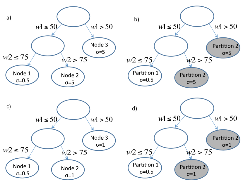
Each simulation study involves five covariates $W_{1}\ldots W_{5}$, each of which is a discrete uniform variable on the integers 1-100. Only $W_{1}$ and $W_{2}$ influence survival times; these are generated from an exponential distribution with a covariate-dependent mean parameter $\sigma$. We consider both a “high” and ‘low” signal setting. In the high signal scenario, $\sigma$ is set equal to 5 if $W_{1}>50$ or $W_{2}>75$ and 0.5 otherwise; in the low signal scenario, the values for $\sigma$ are 1 and 0.5 respectively.

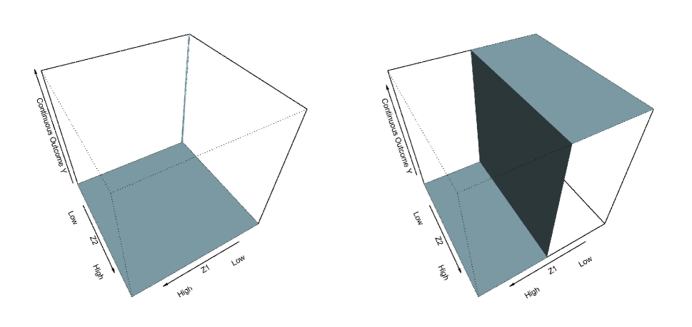
Importantly, there is a single true regression model in each study having two correct regression tree representations. The true CART tree structure has three terminal nodes; however, two of these nodes represent distinct subpopulations of subjects having the same survival distribution. In contrast, the true partDSA tree has two terminal partitions, combining these two terminal nodes into a single partition (i.e., a more parsimonious representation). Figure 1 summarizes these representations for both the high and low signal settings.

In each study, censoring times are independently generated from uniform distributions. For each signal level, two censoring settings are considered. In the first setting, censoring is allowed to depend on covariate information, such that an (approximately) equal level of censoring exists in both risk groups that is close to the specified nominal level. In the second setting, censoring is generated independently of all covariate information, such that overall censoring levels approximately match the specified nominal level. Censoring probabilities used in the calculation of censoring weights are respectively estimated using survival curves derived from an incorrectly specified Cox regression model (i.e., the correct variables are included, but not modeled correctly) and a properly specified nonparametric product-limit estimate of survival. To ensure these estimated censoring probabilities remain bounded away from zero, observed survival times are truncated using a sample-dependent truncation time, as described in Web Appendix B. The actual censoring level decreases slightly after truncation; therefore, both nominal and empirical levels are reported.

Below, we only report results for the setting of covariate-dependent censoring in Section 3.2, where censoring probabilities are estimated using Cox regression. Important performance differences in the setting of covariate-independent censoring are highlighted; figures and tables referenced but not found in the main document may be found in Web Appendix C. Notably, since $CART_{IPCW}$ and $\emph{partDSA}_{IPCW}$ use the same loss function, a direct comparison of these results illustrates the difference between the partDSA and CART algorithms, controlling for both censoring type and level. However, before giving these results, we first describe the metrics that will be used to evaluate prediction performance in the test set.

Figure 1: True Models for Multivariate Simulations of Section 3.2. Panel (a): High Signal: CART representation. Panel (b): High Signal: partDSA representation. Panel (c): Low Signal: CART representation. Panel (d): Low Signal: partDSA representation.

3.1 Test Set Evaluation Criteria

Performance evaluations are based on four criteria: prediction concordance, prediction error, proper risk stratification, and pairwise predictive similarity. In each case, we intend to evaluate how well a model built using censored data performs on an independent, fully observed test set (i.e., no censoring). For brevity, we use “tree” and “terminal node” to describe the structure and output for both partDSA and CART in this section, with the understanding that the true meanings do differ somewhat for partDSA. Below, a brief description of each measure is given; a detailed description of each measure may be found in Web Appendix C.

Prediction Concordance ($C_{p},~{}\bar{C}_{p}$): To ensure comparability across the different methods of tree construction, we define prediction concordance using the terminal-node-specific IPCW-estimated average survival time derived from the training set data as the predicted outcome. Observed and predicted outcomes for subjects in the test set are then compared using the concordance index $C_{p}$ (Harrell et al., 1982) and a modification $\bar{C}_{p}$ suggested in Yan and Greene (2008) that typically exhibits less bias in settings where ties between predicted values are possible. Values near 1.0 (0.5) indicate excellent (poor) concordance.

Prediction Error ($L_{p}$): In this method of evaluation, we compare for each method the predictions for each test set subject obtained using the true tree structure (cf. Figure 1) and the corresponding estimated tree structure. The average squared error of the difference in these predictions, $L_{p},$ equals zero if and only if both trees classify all test set subjects into the same risk groups, and increases away from zero as the heterogeneity in risk group assignment, hence predicted risk, increases.

Pairwise Prediction Similarity ($D_{p}$): This criterion, motivated by work in Chipman et al. (2001), targets the ability of each method to identify groups of subjects having a similar level of risk. In particular, considering all possible pairings of subjects, this measure looks at the extent to which each true tree and corresponding set of estimated trees classify pairs of subjects into the same risk groups. With perfect agreement, $D_{p}=1$; with perfect disagreement, $D_{p}=0$. An advantage of this metric is its independence from both tree topology and the actual predictions associated with each terminal node.

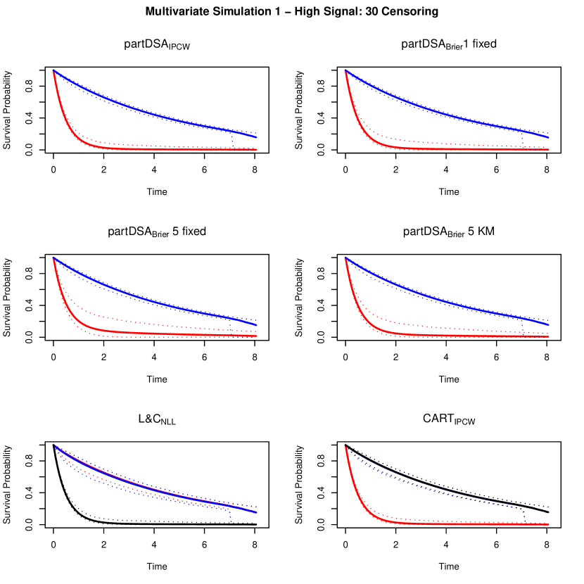
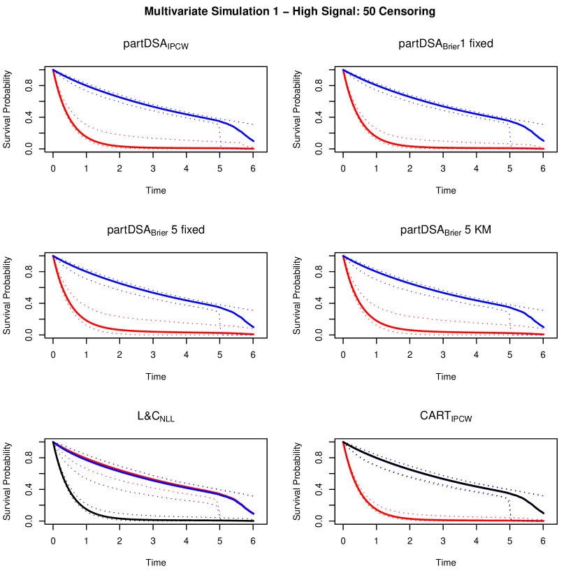
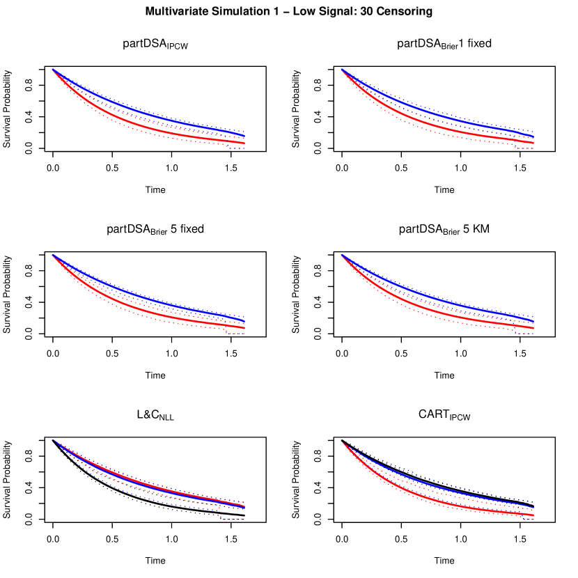
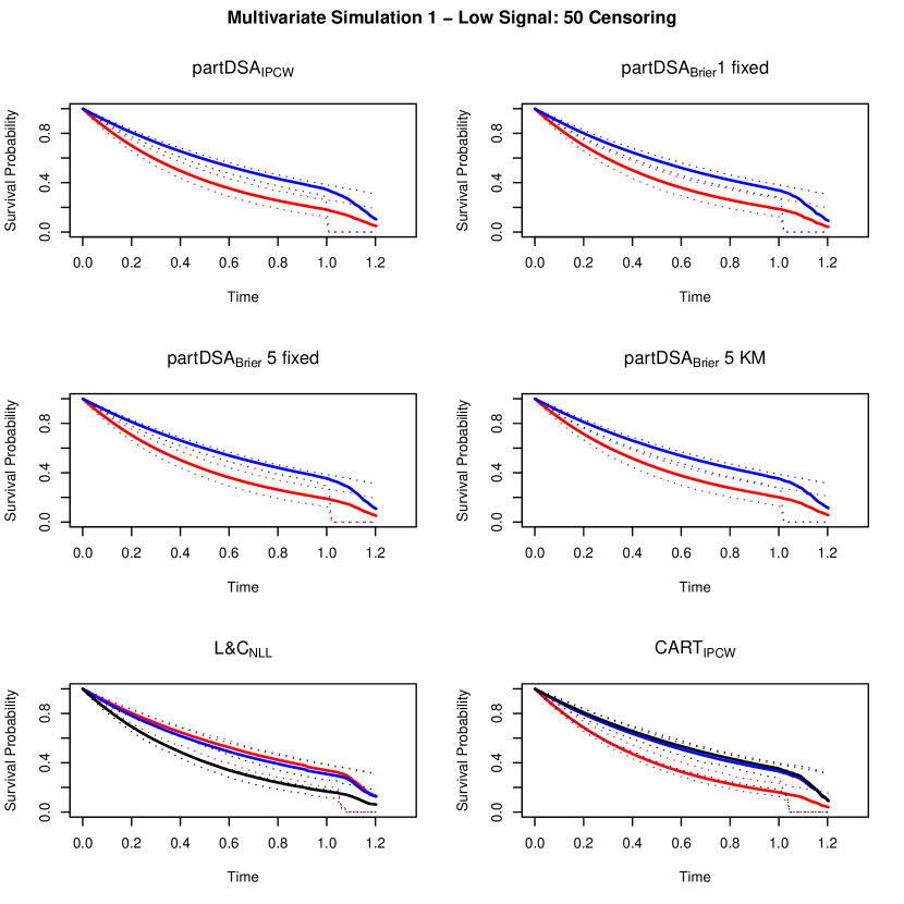
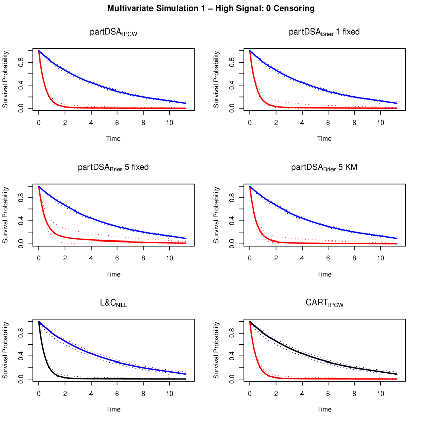
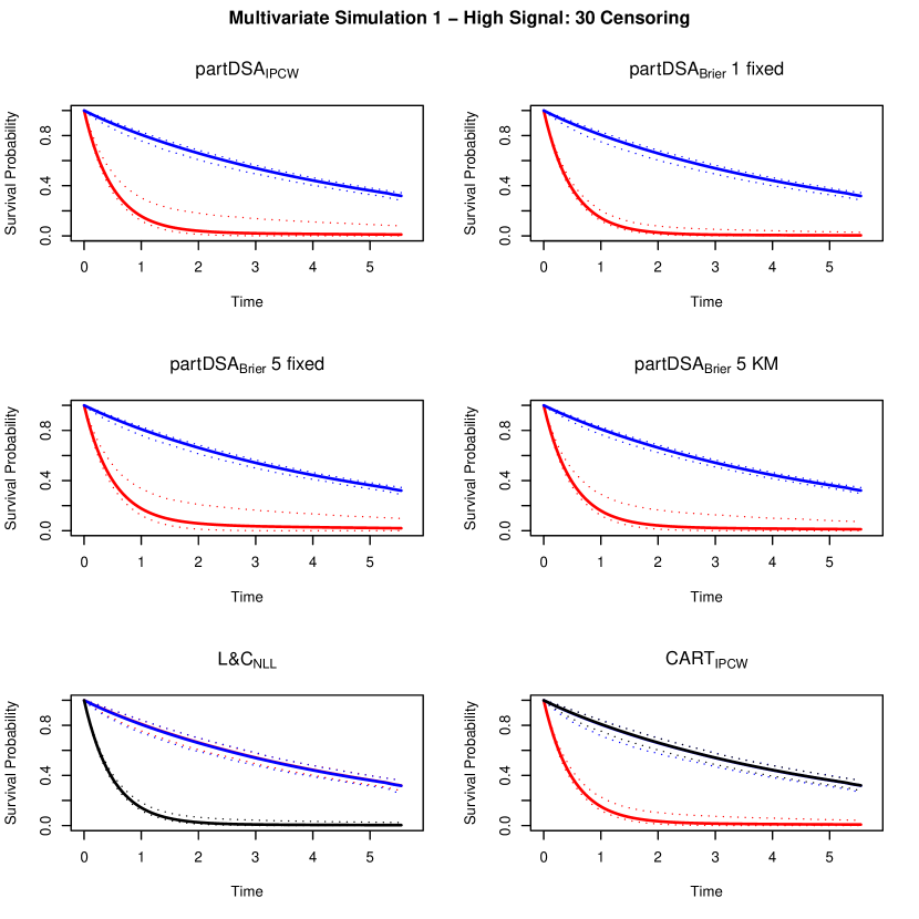
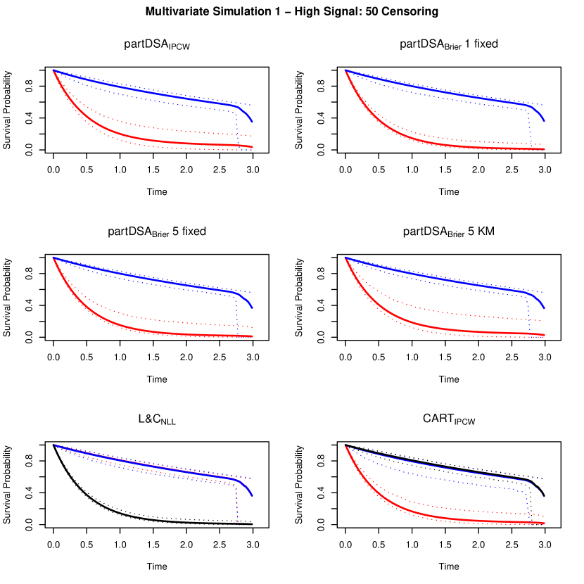
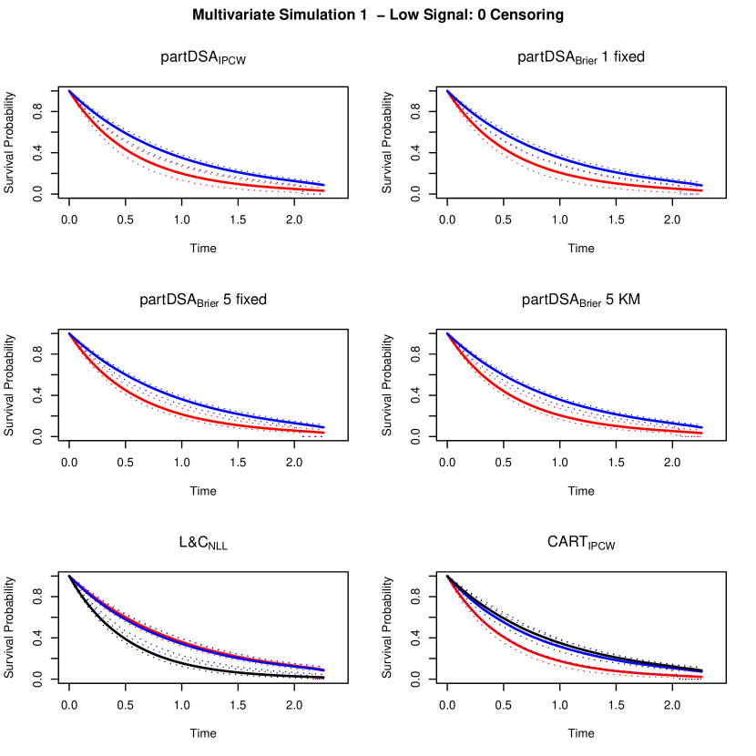
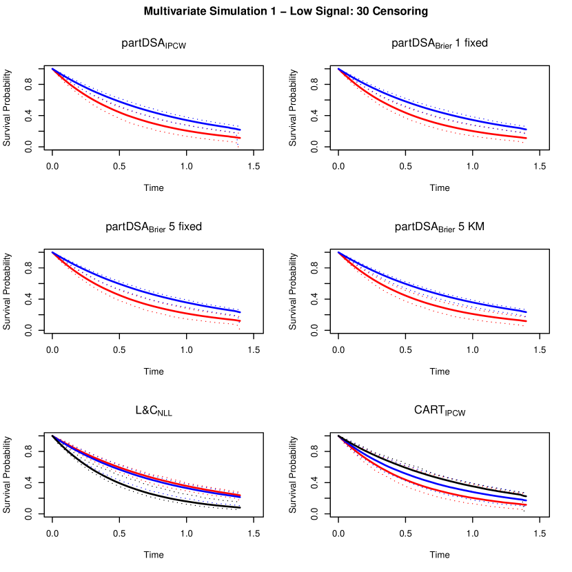
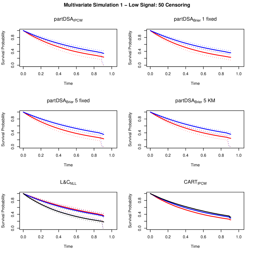
Risk Stratification: This criterion also focuses on the ability to properly separate patients into groups of differing risk. In particular, for each of the 1000 independent test sets, node-specific empirical survivor functions are computed. Then, for each estimation method, and for the subset of the 1000 estimated trees that consist of either two or three terminal nodes, we compute the corresponding empirical survivorship and 0.025 and 0.975 percentiles on a fine grid of time points. A graphical summary of the results is provided for each simulation study. As suggested by Figure 1, we expect to see a high proportion of cases for partDSA (CART) with only two (three) survival curves and smaller (larger) standard errors.

3.2 Results

As seen in Table 1, all methods build slightly larger models than necessary while selecting the two signal variables consistently. Overall, $\emph{partDSA}_{Brier}(5even)$ and $\emph{partDSA}_{IPCW}$ exhibit the best performance on the evaluation metrics introduced in Section 3.1, with $\emph{partDSA}_{IPCW}$ also consistently outperforming $\emph{CART}_{IPCW}.$

In general, c-indices are comparable, with the partDSA methods doing as well, and usually better, than the CART-based methods. The relative improvement in performance based on the mean c-index ranges up to 6%, with the greatest improvement being seen at the highest censoring level. In addition, $\emph{partDSA}_{IPCW}$ and $\emph{partDSA}_{Brier}(5KM)$ have the lowest prediction error in the presence of censoring, with $\emph{partDSA}_{IPCW}$ having the lowest prediction error for $0\%$ and $30\%$ censoring and $\emph{partDSA}_{Brier}(5KM)$ having the lowest error in the case of $50\%$ censoring. In comparison with the CART-based methods, the relative decrease in prediction error ranges up to $53\%.$ In comparison with CART-based methods, the partDSA methods also perform approximately $15\%$ better on the pairwise prediction similarity measure. Web Figures  4-6 depict the average empirical survival curves for the four methods, where the partDSA and CART methods routinely identify two and three distinct groups of patients, respectively; see Web Table 1). However, in the case of CART, the clinical utility of these three risk groups is not as apparent, for two of these groups are estimated to have nearly identical survival experiences, each having wider standard errors.

In general, some variation in performance is observed across the different choices of Brier score loss function, with $\emph{partDSA}_{Brier}(5KM)$ consistently performing well on all four metrics, followed by $\emph{partDSA}_{Brier}(1Fixed)$ and then $\emph{partDSA}_{Brier}(5even).$ The difference in performance between $\emph{partDSA}_{Brier}(5KM)$ and $\emph{partDSA}_{Brier}(5even)$ is noticeable and cannot be explained by the introduction of censoring, for the performance of both is reasonably stable for each metric across censoring levels. This is less true for $\emph{partDSA}_{Brier}(1Fixed),$ where more substantial changes in prediction error and pairwise predictive similarity are observed with increasing levels of censoring.

Table 1: Simulation Results: High Signal, Covariate-Dependent Censoring. Reported are true and average fitted model sizes, number of predictors in the fitted model, number of correct (incorrect) predictors selected, c-index ratios ($C_{p}$, $\bar{C}_{p}$; larger values indicate better performance), prediction error ($L_{p}$; smaller values indicate less error), and pairwise prediction similarity error ($D_{p}$; larger values indicate less error) for the four methods over three censoring levels for the simulation. The $1Fixed$ method refers to $\emph{partDSA}_{Brier}$ using a single fixed time point; the $5even$ method refers to $\emph{partDSA}_{Brier}$ using 5 evenly spaced time points; and, the $5KM$ method refers to $\emph{partDSA}_{Brier}$ using 5 time points determined using percentiles of the Kaplan-Meier estimate of the marginal survivor function.

		$\emph{partDSA}_{Brier}$			IPCW
Censoring	Criteria	$1Fixed$	$5Even$	$5KM$	partDSA	$CART$	$L\&C_{NLL}$
	True Model Size	2.00	2.00	2.00	2.00	3.00	3.00
$0\%$/$0\%$	Fitted Size	2.198	2.450	2.228	2.170	3.106	3.192
	# Predictors	2.135	2.095	2.195	2.111	2.047	2.076
	# W1-W2	1.998	1.809	2.000	1.999	1.962	1.996
	# W3-W5	0.137	0.286	0.195	0.112	0.085	0.080
	$C_{p}$	0.879	0.828	0.880	0.891	0.812	0.809
	$\bar{C}_{p}$	0.782	0.748	0.783	0.789	0.748	0.747
	$L_{p}$	0.082	0.270	0.076	0.061	0.076	0.072
	$D_{p}$	0.944	0.838	0.946	0.964	0.845	0.842
$30\%$/$26.4\%$	True Size	2.000	2.000	2.000	2.000	3.000	3.000
	Fitted Size	2.249	2.391	2.227	2.230	3.058	3.222
	# Predictors	2.190	2.160	2.206	2.146	1.988	2.090
	# W1-W2	1.993	1.894	2.000	1.999	1.904	1.988
	# W3-W5	0.197	0.266	0.206	0.147	0.084	0.102
	$C_{p}$	0.867	0.839	0.878	0.881	0.810	0.802
	$\bar{C}_{p}$	0.775	0.756	0.783	0.784	0.744	0.742
	$L_{p}$	0.125	0.225	0.084	0.082	0.126	0.118
	$D_{p}$	0.918	0.857	0.940	0.944	0.828	0.825
$50\%$/$45.7\%$	True Size	2.000	2.000	2.000	2.000	3.000	3.000
	Fitted Size	2.396	2.361	2.251	2.359	2.937	3.093
	# Predictors	2.137	2.136	2.200	2.191	1.875	1.983
	# W1-W2	1.908	1.888	1.997	1.974	1.802	1.881
	# W3-W5	0.229	0.248	0.203	0.217	0.073	0.102
	$C_{p}$	0.845	0.844	0.874	0.864	0.810	0.794
	$\bar{C}_{p}$	0.761	0.759	0.781	0.775	0.740	0.732
	$L_{p}$	0.199	0.216	0.102	0.125	0.188	0.215
	$D_{p}$	0.862	0.855	0.926	0.906	0.805	0.792

There is greater heterogeneity in the performance comparison for the case of covariate-independent censoring; see Web Table  3. Noteworthy observations include (i) a consistent dominance of the CART-based method $L\&C_{NLL}$ on the prediction error metric in the presence of censoring; (ii) the consistent and generally high level of performance of $\emph{partDSA}_{Brier}(5KM)$ on all metrics; and, (iii) the continued dominance of $\emph{partDSA}_{IPCW}$ over $\emph{CART}_{IPCW}$ on all metrics regardless of censoring level, despite a more noticeable degradation in performance on the prediction error and pairwise predictive similarity indices as censoring increases in comparison with Table 1.

The results of the low signal simulation are summarized in Table 2. All methods select models less than the ideal size, choosing fewer correct W1-W2 variables, though still with greater frequency in comparison with the incorrect W3-W5 variables. Further information on chosen model sizes may be found in Web Table 2. In general, the partDSA methods perform similarly to the CART methods on all four performance metrics; however, relative to CART, moderate improvement is observed at the 50% censoring level on all metrics for $\emph{partDSA}_{IPCW}$ and $\emph{partDSA}_{Brier}(5Even).$ Empirical survival curves are summarized in Web Figures 7–9, where patterns are generally similar to those reported earlier. Similar results are observed in the case of covariate-independent censoring, though the improvement observed at the 50% censoring level in the high signal setting is no longer evident; see Web Tables 5 and 6 and Web Figures 13 –15.

Table 2: Simulation Results: Low Signal, Covariate-Dependent Censoring. Reported are true and average fitted model sizes, number of predictors in the fitted model, number of correct predictors selected, c-index ratios ($C_{p}$, $\bar{C}_{p}$; larger values indicate better performance), prediction error ($L_{p}$; smaller values indicate less error), and pairwise prediction similarity error ($D_{p}$; larger values indicate less error) for the four methods over three censoring levels for the simulation. The $1Fixed$ method refers to $\emph{partDSA}_{Brier}$ using a single fixed time point; the $5even$ method refers to $\emph{partDSA}_{Brier}$ using 5 evenly spaced time points; and, the $5KM$ method refers to $\emph{partDSA}_{Brier}$ using 5 time points determined using percentiles of the Kaplan-Meier estimate of the marginal survivor function.

		$\emph{partDSA}_{Brier}$			IPCW
Censoring	Criteria	$1Fixed$	$5Even$	$5KM$	partDSA	$CART$	$L\&C_{NLL}$
	True Model Size	2.00	2.00	2.00	2.00	3.00	3.00
$0\%$/$0\%$	Fitted Size	1.642	1.502	1.389	1.456	1.590	1.873
	# Predictors	0.705	0.521	0.496	0.586	0.571	0.838
	# W1-W2	0.621	0.471	0.410	0.491	0.527	0.786
	# W3-W5	0.084	0.050	0.086	0.095	0.044	0.052
	$C_{p}$	0.608	0.604	0.602	0.607	0.603	0.610
	$\bar{C}_{p}$	0.567	0.562	0.559	0.563	0.563	0.571
	$L_{p}$	0.080	0.086	0.091	0.087	0.083	0.071
	$D_{p}$	0.618	0.592	0.581	0.600	0.608	0.644
$30\%$/$26.7\%$	Fitted Size	1.550	1.536	1.290	1.456	1.571	1.546
	# Predictors	0.676	0.648	0.427	0.705	0.553	0.523
	# W1-W2	0.575	0.527	0.319	0.551	0.517	0.473
	# W3-W5	0.101	0.121	0.108	0.154	0.036	0.050
	$C_{p}$	0.607	0.604	0.597	0.611	0.607	0.607
	$\bar{C}_{p}$	0.565	0.562	0.554	0.565	0.565	0.563
	$L_{p}$	0.073	0.076	0.084	0.076	0.073	0.075
	$D_{p}$	0.607	0.591	0.565	0.605	0.609	0.597
$50\%$/$45.7\%$	Fitted Size	1.648	1.780	1.306	1.591	1.572	1.282
	# Predictors	0.812	1.106	0.533	0.943	0.552	0.264
	# W1-W2	0.659	0.911	0.375	0.758	0.513	0.233
	# W3-W5	0.153	0.195	0.158	0.185	0.039	0.031
	$C_{p}$	0.607	0.616	0.602	0.614	0.607	0.601
	$\bar{C}_{p}$	0.566	0.574	0.556	0.570	0.565	0.555
	$L_{p}$	0.056	0.049	0.066	0.055	0.058	0.067
	$D_{p}$	0.609	0.649	0.571	0.629	0.608	0.562

4 Data Analysis

We now illustrate the model building capabilities of partDSA- and CART-based methods using data from 12 North American Brain Tumor Consortium (NABTC) Phase II clinical trials for recurrent glioma (Wu et al., 2010), run to assess the efficacy of novel therapeutic agents in patients with grade III or IV gliomas. As there are few efficacious treatments for high-grade glioma and median survival is low (14.6 months; Stupp et al., 2005), there is strong interest in identifying prognostic factors associated with overall survival. Recently, several studies have combined data from multiple (necessarily small) Phase II clinical trials to examine such factors using a various statistical methods; however, findings have at best been moderately consistent (Wong et al., 1999; Carson et al., 2007; Wu et al., 2010).

Wu et al. (2010) combined the NABTC data with 15 North Central Cancer Treatment Group (NCCTG) trials and found tumor grade, patient age, baseline performance score, and time since diagnosis as important prognostic variables. Based on these results and those of earlier studies, Wu et al. (2010) conclude that there is strong evidence to suggest that future trials should collect and report this information as predictors of patient prognosis. Limitations of these analyses, and those to be presented below, include the possibility of trial referral bias and biases induced as a result of variation in patient eligibility criteria across studies.

The NABTC data set analyzed here includes 549 patients that were treated on Phase II trials between February 1998 and December 2002 (Wu et al., 2010); Web Table LABEL:T:Glioma summarizes the data on 18 variables that include age, gender and several variables documenting a patient’s health and tumor status as well as current/past therapies. The outcome of interest is overall survival (OS), defined as time from study registration date to the date of death due to any cause (median OS was 30.4 weeks). Thirty patients were censored at last follow-up date, being still alive or lost to follow-up. There are several noteworthy differences between the analysis and results here and in Wu et al. (2010). First, many of the results in that paper refer to the combined analysis of 27 trials, not just the 12 trials considered here; in addition, and important to the motivation for our analysis, is the fact that the risk groups ultimately identified in Wu et al. (2010, Table 5) were determined by post-processing the results of their analyses in a subjective and relatively ad hoc manner. In particular, their primary analysis consisted of estimating the cumulative hazard function for OS using a Cox proportional hazard model adjusted only for current temozolomide (TMZ) use and then subsequently analyzing this predicted count using CART without any further accounting for censoring. In subsequent analysis, logrank tests were used to test for pairwise differences between terminal nodes; terminal nodes were then combined for the purposes of defining risk groups if the p-value from a corresponding log-rank test was $>0.01$ (Wu et al., 2010, Table 5). That is, Wu et al. (2010) form risk groups using a combination of ’and’ statements derived from CART and ’or’ statements created using the indicated testing procedure. Important differences between their approach and partDSA include an improper accounting for censoring, a lack of objectivity in the methodology used for defining risk groups, and the failure to use cross-validation in evaluating the final models.

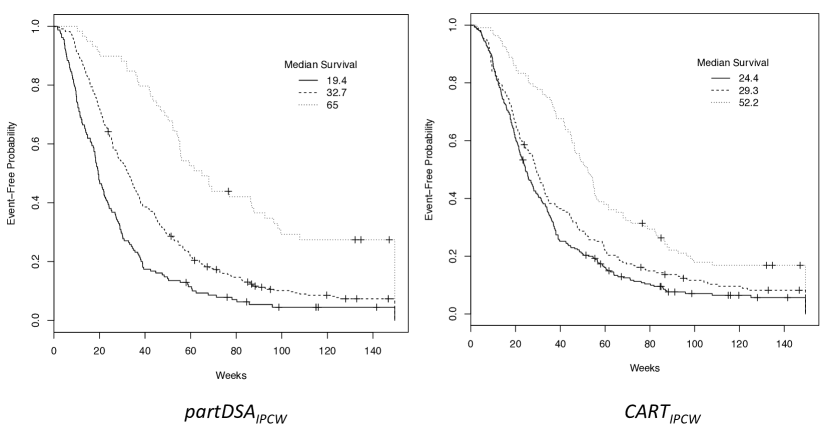
All four algorithms from Sect. 3 were run using 10-fold cross-validation; below, we summarize the results from $partDSA_{Brier}(5KM)$ and $L\&C_{NLL}$, with further discussion of the remaining results in Web Appendix D. The risk stratification determined by $partDSA_{Brier}(5KM)$ is based on Karnofsky performance score (KPS; a marker for overall tumor burden and cumulative treatment-related toxicity), patient age, time since diagnosis, baseline steroid use, gender, prior TMZ therapy (an approved treatment for recurrent gliomas), and current TMZ therapy. Three primary risk groups are identified; these are depicted in Table 3, with corresponding survival experiences summarized by Kaplan-Meier curves in the left panel of Figure 2. The low, medium and high risk groups respectively have median survival times of 55.6 weeks (144 patients), 32.3 weeks (218 patients), and 19.7 weeks (187 patients); see Table 3. In a sub-analysis of the NABTC data, Wu et al. (2010, Table 7) found the same first five variables using a predicted outcome variable that adjusts for current TMZ therapy. Hence, the only difference in the variables selected is the inclusion of prior TMZ use; this clinically relevant variable indicates that a patient previously failed TMZ therapy, lessening the chances of successful treatment.

For comparison, Table 4 and Figure 2 (right panel) summarize the corresponding results for $L\&C_{NLL}$. It is observed that $L\&C_{NLL}$ selects only two of the variables identified by $partDSA_{Brier}(5KM)$ (i.e. age split at 55 and prior TMZ), but creates three risk groups. The lowest risk group is defined by younger patients without prior TMZ treatment (median survival of 46.3 weeks, 176 patients); the highest risk group is defined by older patients (median survival of 25.3 weeks, 195 patients). The two groups at higher risk are also observed to have very similar survival experiences, and the estimated spread in median survival times is approximately 15 weeks shorter for $L\&C_{NLL}.$ With the exception of the low risk group, the reported 95% confidence intervals for median survival times associated with the Kaplan-Meier curves for $partDSA_{Brier}(5KM)$ are also considerably tighter than those associated with the risk groups identified by $L\&C_{NLL}.$ Arguably, the separation in risk identified here is not as clinically relevant as that found by partDSA. We note here that the 95% confidence intervals presented in these two tables are only meant to provide a sense of variability; because of the post-hoc manner in which they are obtained, such intervals are not expected to have the correct frequentist coverage. Further comments and comparisons to results in Wu et al. (2010) may be found in Web Appendix D.

Table 3: $partDSA_{Brier}(5KM)$ stratification of NABTC patients (Sect. 4) into three risk groups (column 1: low, intermediate (Int), and high). Corresponding median survival in weeks and 95% confidence intervals (CI) are given in column 2 and number of patients in each group in column 3. Variables included in the model (columns 4–10) are Karnofsky performance score (KPS), age, current TMZ, time since diagnosis (Dx), prior TMZ, baseline steroid use (steroid), and gender.

			Variables
Risk	Median survival	$n$			Current	Time Since	Prior
Group	(95% CI)	(549)	KPS	Age	TMZ	Dx	TMZ	Steroid	Gender
Low		144	$\geq 90$	$\leq 55$			No
	55.6		$\leq 80$		No			No	Female
	(48.6, 66.3)		$\leq 80$		Yes	$\leq 16.9$
			$\leq 80$		Yes	$(24,33.7]$
Int.		218	$\geq 90$				Yes
	32.3		$\geq 90$	$>55$			No
	(28.1, 36.9)		$\leq 80$		Yes	$<33.7$
High		187	$\leq 80$		No			Yes
	19.7		$\leq 80$		No			No	Male
	(18.3, 21.9)		$\leq 80$		Yes	$(16.9,24]$

Figure 2: Kaplan-Meier Curves for NABTC data analysis in Section 4.

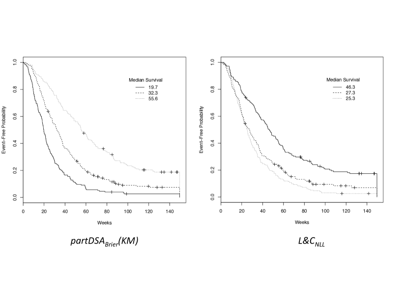
Left panel: $partDSA_{Brier}(5KM)$ stratification of patients into three risk groups. Right panel: $L\&C_{NLL}$ stratification of patients into three risk groups.

Table 4: $L\&C_{NLL}$ stratification of NABTC patients (Sect. 4) into three risk groups (column 1: low, intermediate (Int), and high). Corresponding median survival in weeks and 95% confidence intervals (CI) are given in column 2 and number of patients in each group in column 3. Variables included in the model (columns 4–5) are age and prior TMZ.

Risk	Median survival	$n$	Variables
Group	(95% CI)	(549)	Age	Prior TMZ
Low	46.3 (40.9, 54.7)	176	$\leq 55$	No
Intermediate	27.3 (22.3, 33.3)	177	$\leq 55$	Yes
High	25.3 (21.7, 28.3)	196	$>55$

In earlier analyses of other glioma studies, Wong et al. (1999) found histologic diagnosis at study registration (i.e., grade), prior treatment(s), and KPS to be associated with overall survival, whereas Carson et al. (2007) noted initial histology (GBM vs other; i.e., grade), age, KPS, baseline steroid use, shorter time from original diagnosis to recurrence, and tumor outside frontal lobe to be prognostic. As implied in earlier discussion, Wu et al. (2010) found grade to be important in the recursive partitioning analysis of the NCCTG trials alone and also in combination with the NABTC trials; however, grade was not identified as being prognostic when looking only at the NABTC trials. In combination with our own analyses of the NABTC trial data, we conclude that prior TMZ therapy, baseline steroid use, and gender should be incorporated into the set of variables that Wu et al. (2010) recommend for consideration when planning future clinical trials of high-grade glioma patients.

5 Discussion

The ability to successfully build a model for predicting a survival outcome has important clinical implications. Censored survival outcomes have inherent challenges compared to continuous and categorical outcomes; the development of tree-based methods for analyzing survival data deserves further attention and study. We have introduced two methods for extending partDSA to right-censored outcomes: the IPCW and Brier Score weighting schemes. In simulation studies, these two methods are observed to perform as well, and often considerably better, than either $CART_{IPCW}$ or $L\&C_{NLL}$ using several distinct evaluation criteria. As illustrated in Figure 1, greater stability can be expected from the partDSA representation since fewer terminal partitions are needed to represent distinct groups of subjects with similar levels of risk.

The $partDSA_{Brier}$ methodology holds clear promise for risk stratification on the basis of survival probabilities, particularly so the “integrated” (i.e., composite loss) versions. Compared with the two other IPCW-$L_{2}-$loss based methods, $partDSA_{Brier}$ maintains good performance for higher censoring levels. In part, we attribute this good behavior to both a sensible target of estimation and the calculation of IPC weights at time points bounded away from the tail of the survivor distribution. The $partDSA_{Brier}$ methods also make better use of the available failure time information by including both observations that are uncensored and censored after a specified time cutpoint; whereas IPCW (for both algorithms) only directly includes uncensored observations. This additional utilization of information may reduce the variability in the estimated loss functions, resulting in improved performance; see Strawderman (2000) for related discussion. Finally, the “integrated” (i.e., composite loss) version of the Brier score loss function has two useful robustness properties: invariance to monotone transformations of time; and, strong connections to estimating median, rather than mean, survival (Lawless and Yuan, 2010, Theorem 1). As a result, the performance of $partDSA_{Brier}$ as a risk stratification procedure is less likely to be influenced by the presence of a few extreme response values.

Although partDSA has advantages over CART, one important fixed disadvantage is its greater computational burden. In particular, because partDSA iterates among three possible moves and performs an exhaustive search of the covariate space, it will inevitably require a significantly higher running time than CART. The R package for partDSA allows for the cross-validation folds to be run in parallel, making runnings time feasible in many applications (Molinaro et al., 2010), especially given that most clinical datasets remain relatively modest in size. In future work, we will look further at variable selection in partDSA and corresponding variable importance measures. Such extensions will serve to further improve the already-demonstrated potential of partDSA.

6 Supplementary Materials

Web Appendices, Tables, and Figures referenced in Sections 2 – 4 are available at the end of this paper.

Web Appendix A: Further detail on partDSA

partDSA utilizes three moves, or step functions, to generate index sets (i.e., different partitionings of the covariate space) with the goal of minimizing a risk function over all the generated index sets. These three moves include:

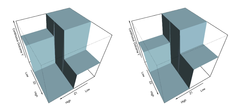
• Deletion: A deletion move forms a union of two regions of the covariate space regardless of their spatial location, i.e., the two regions may not be contiguous. An example is shown in Figure 1.

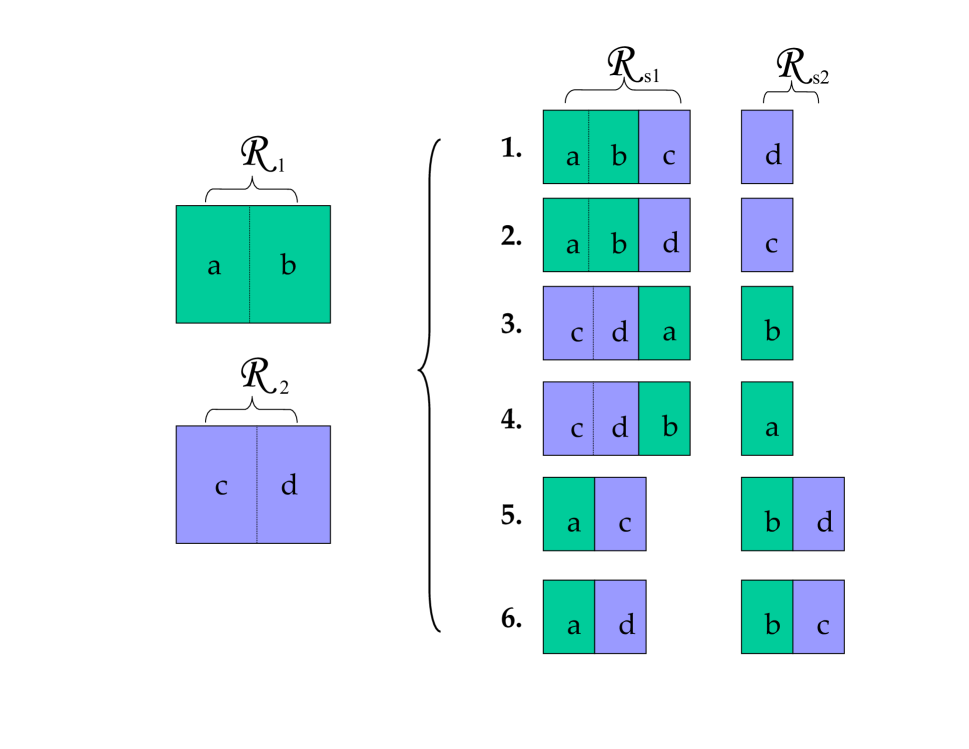
• Substitution: A substitution move divides two disparate regions into two subsets each and then forms combinations of the four subsets resulting in two new regions. Thus, this step forms unions of regions (or subsets within the regions) as well as divides regions. The possible subsets of two regions and combinations thereof can be seen in Figure 2.

• Addition: An addition move splits one region into two distinct regions. An example is shown in Figure 3.

Figure 1: Two dimensional display of Deletion Step. Two disparate regions on the left form a union on the right. This union reads: ”If low on Z1 and high on Z2 OR low on Z2 and high on Z1.”

Figure 2: Possible Substitution Moves for two disparate regions. The ’best’ split on Region 1 ($\mathcal{R}_{1}$) is found and labeled $a$ and $b$. The ’best’ split on Region 2 ($\mathcal{R}_{2}$) is found and labeled $c$ and $d$. All (six) unique combinations of $a,b,c,\mbox{ and }d$ are formed as $R_{s1}$ and $R_{s2}$.

Figure 3: Two dimensional display of Addition Step. The algorithm is initiated on the left and the ’best’ split is found separating ’low’ on Z1 from ’high’.

Web Appendix B: Computational Details For Simulation Studies

The rpart package version 3.1-49 available in R was used for the $L\&C_{NLL}$ method, and code from Molinaro et al. (2004), also based on rpart, for $CART_{IPCW}$. The default tuning parameters were used for rpart except as noted below. In partDSA, version 0.8.2 (available on R-forge), $MB$, defined as the minimum number of observations per “or” statement was set to 15. In rpart, $minbuck$, the minimum number of observations per node was set to 15. To allow both algorithms the opportunity to build the same size models we set rpart’s $minsplit$ to 30. The minimum percent difference ($MPD$) in partDSA is a threshold for the required improvement in the risk to make a particular move (e.g., deletion) and was set to 0.05. Additionally, both algorithms were restricted to a max of 10 nodes or partitions. Five-fold cross validation was carried out in a standardized way for all methods such that the partition of the observations into the five folds was identical for each method.

As indicated in the main document, the observed survival times are truncated to help ensure estimated censoring probabilities remain bounded away from zero. Specifically, we set the sample-dependent truncation time $\tau$ such that the proportion of observed follow-up times exceeding $\tau$ is 5% of the total sample size. All follow-up times exceeding $\tau$ are set equal to $\tau$ and are subsequently considered uncensored. Consequently, all truncated survival times lie in $(0,\tau]$.

In the case of $\emph{partDSA}_{Brier},$ a vector of times for loss computation must be chosen. As described in the main paper, we simply used the theoretical median of the marginal survivor function computed under the specified model in the case of $\emph{partDSA}_{Brier}(1Fixed).$ In the case of $\emph{partDSA}_{Brier}(5Even)$ and $\emph{partDSA}_{Brier}(5KM),$ a sample-dependent vector of 5 time points is used. For $\emph{partDSA}_{Brier}(5Even),$ we select the time points $(j/6)\tau$ for $j=1,2,3,4,5$; for $\emph{partDSA}_{Brier}(5KM),$ we compute the Kaplan-Meier estimate of the marginal survivor function and then use the times that respectively correspond to survival probabilities of 0.85, 0.7, 0.55, 0.40 and 0.25. The loss $BS^{c}(t)$ in (2) is then computed for each of the 5 time points in both cases and aggregated to obtain a composite measure of loss. In particular, if $t_{1}<t_{2}<t_{3}<t_{4}<t_{5}$ denote these 5 time points, we compute the weighted average loss:

$$B^{*}=\sum_{i=1}^{5}|\frac{t_{i}}{t_{5}}|BS^{c}(t_{i}),$$

the weight $|t_{i}/t_{5}|$ serving to emphasize later survival differences over earlier differences (and the absolute value allowing for the possibility of times on the log scale); see Graf et al. (1999) for further discussion.

Web Appendix C: Extended Detail for Multivariate Simulation Studies

C.1: Detailed Description of Evaluation Measures

Prediction Concordance: To ensure comparability across the different methods of tree construction, we define prediction concordance using the terminal-node-specific IPCW-estimated average survival time derived from the training set data as the predicted outcome. For each test set, all members are classified into a terminal node for each estimated tree based only on their covariates and assigned a corresponding estimated average survival time as their predicted outcome. The concordance index, or c-index, compares observed and predicted outcomes for each method in each test set by computing the fraction of pairs in which the observation having the shorter event time also has the shorter model-predicted event time (Harrell et al., 1982). Since it is possible (indeed, expected) that test subjects with different outcomes will have tied predicted values, we report two c-indices, one that excludes all such tied pairs ($C_{p}$) and another that is calculated as the numerical average of this c-index and that calculated including all such tied pairs ($\bar{C}_{p}$). The latter typically exhibits less bias in comparison to measures that respectively exclude and include ties (Yan and Greene, 2008).

Prediction Error: In this method of evaluation, two predicted outcomes are computed for each test set member for each estimation method. First, a predicted outcome is determined by running all test set subjects down the true partDSA tree and then again down the corresponding CART tree (cf. Figure 1). The predicted outcome for subject $i$, say $\psi^{TT}_{i},$ is taken to be the average survival time of all members assigned to the same terminal node. The second predicted outcome is determined in exactly the same fashion, but instead runs each test set member down the estimated tree built using the training set; call this predicted outcome $\psi^{TS}_{i}.$ Comparing predictions over all subjects measures how well the estimated tree (i.e., structurally speaking) predicts the true subject-specific risk. We measure the distance between these predicted outcomes using $L_{p}=1/5000\sum_{i=1}^{5000}(\psi^{TT}_{i}-\psi^{TS}_{i})^{2}.$ Evidently, $L_{p}=0$ if and only if both trees classify all test set subjects into the same risk groups, and increases away from zero as the heterogeneity in risk group assignment, hence predicted risk, increases.

Risk Stratification: This criterion focuses on the ability of each method to properly separate patients into groups of differing risk. In particular, for each of the 1000 independent test sets, node-specific empirical survivor functions are computed. Then, for each estimation method, and for the subset of the 1000 estimated trees that consist of either two or three terminal nodes, we computed the corresponding average survivorship and 0.025 and 0.975 percentiles on a fine grid of time points. A graphical summary of the results is provided for each simulation study. For partDSA, we expect to see a high proportion of cases with only two risk groups (i.e., survival curves) and small standard errors. For CART, we expect to observe a high proportion of cases with three risk groups, with two of these groups representing subpopulations having identical survival distributions and corresponding estimates that consequently reflect greater levels of error.

Pairwise Prediction Similarity: This last criterion also examines the separation of patients into risk groups, targeting the ability of each method to identify groups of subjects having a similar level of risk. Given the underlying tree model, the terminal node (hence risk group) for each observation is known. Define $I_{T}(i,j)$ to be 1 if observations $i$ and $j$ are grouped into the same terminal node (i.e., into the same risk group) under this true model and set it equal to 0 otherwise. Then, $I_{T}(i,j)$ is known for each of the ${n\choose 2}$ unique pairs in each test set. For structures estimated by partDSA and CART, we can compute analogous measures of agreement/discrepancy for all unique test set pairs; generically, let this measure be denoted by $I_{M}(i,j).$ Then, $|I_{T}(i,j)-I_{M}(i,j)|>0$ if and only if an estimated tree incorrectly groups observations $i$ and $j.$ Similarly to Chipman et al. (2001), define the distance measure

$$D_{p}=1-\sum_{i=1}^{n}\sum_{j>i}\frac{|I_{T}(i,j)-I_{M}(i,j)|}{{n\choose 2}}$$ (4)

With perfect agreement, $D_{p}=1$; with perfect disagreement, $D_{p}=0$. We report the average value of $D_{p}$ computed over all 1000 test sets. An advantage of this metric is its independence from both tree topology and the actual predictions associated with each terminal node.

C.2: High Signal, Covariate-Dependent Censoring

Figure 4: High Signal, Covariate-Dependent Censoring: Kaplan-Meier plots for six methods to illustrate the survival experience of chosen risk groups (Section 3.2, 0% censoring).

Figure 5: High Signal, Covariate-Dependent Censoring: Kaplan-Meier plots for six methods to illustrate the survival experience of chosen risk groups (Section 3.2, 30% censoring).

Figure 6: High Signal, Covariate-Dependent Censoring: Kaplan-Meier plots for six methods to illustrate the survival experience of chosen risk groups (Section 3.2, 50% censoring).

Table 1: High Signal, Covariate-Dependent Setting: proportion of the 1000 models at each given size for each method at the three censoring levels.

	Root Node	2	3	4+
0Cens
$L\&C_{NLL}$	$0.001$	$0.001$	$0.869$	$0.129$
$CART_{IPCW}$	$0.018$	$0.001$	$0.861$	$0.120$
$\emph{partDSA}_{IPCW}$		$0.862$	$0.117$	$0.021$
$\emph{partDSA}_{Brier}1fixed$		$0.821$	$0.140$	$0.039$
$\emph{partDSA}_{Brier}5even$	$0.017$	$0.625$	$0.281$	$0.077$
$\emph{partDSA}_{Brier}5KM$		$0.830$	$0.148$	$0.022$
30Cens
$L\&C_{NLL}$	$0.004$	$0.003$	$0.829$	$0.164$
$CART_{IPCW}$	$0.047$	$0.002$	$0.823$	$0.128$
$\emph{partDSA}_{IPCW}$		$0.814$	$0.151$	$0.035$
$\emph{partDSA}_{Brier}1fixed$		$0.834$	$0.127$	$0.039$
$\emph{partDSA}_{Brier}5even$	$0.014$	$0.707$	$0.195$	$0.084$
$\emph{partDSA}_{Brier}5KM$		$0.817$	$0.143$	$0.040$
50Cens
$L\&C_{NLL}$	$0.043$	$0.029$	$0.783$	$0.145$
$CART_{IPCW}$	$0.094$	$0.010$	$0.785$	$0.111$
$\emph{partDSA}_{IPCW}$	$0.001$	$0.728$	$0.205$	$0.066$
$\emph{partDSA}_{Brier}1fixed$	$0.001$	$0.813$	$0.146$	$0.040$
$\emph{partDSA}_{Brier}5even$	$0.035$	$0.694$	$0.183$	$0.088$
$\emph{partDSA}_{Brier}5KM$	$0.021$	$0.702$	$0.186$	$0.091$

C.3: Low Signal, Covariate-Dependent Censoring

Figure 7: Low Signal, Covariate-Dependent Censoring: Kaplan-Meier plots for six methods to illustrate the survival experience of chosen risk groups (Section 3.2, 0% censoring).

Figure 8: Low Signal, Covariate-Dependent Censoring: Kaplan-Meier plots for six methods to illustrate the survival experience of chosen risk groups (Section 3.2, 30% censoring).

Figure 9: Low Signal, Covariate-Dependent Censoring: Kaplan-Meier plots for six methods to illustrate the survival experience of chosen risk groups (Section 3.2, 50% censoring).

Table 2: Low Signal, Covariate-Dependent Setting: Proportion of the 1000 models at each given size for each method at the three censoring levels.

	Root Node	2	3	4+
0Cens
$L\&C_{NLL}$	$0.458$	$0.287$	$0.207$	$0.048$
$CART_{IPCW}$	$0.559$	$0.320$	$0.096$	$0.025$
$\emph{partDSA}_{IPCW}$	$0.635$	$0.290$	$0.062$	$0.013$
$\emph{partDSA}_{Brier}1fixed$	$0.693$	$0.239$	$0.055$	$0.013$
$\emph{partDSA}_{Brier}5even$	$0.584$	$0.343$	$0.062$	$0.011$
$\emph{partDSA}_{Brier}5KM$	$0.522$	$0.336$	$0.121$	$0.021$
30Cens
$L\&C_{NLL}$	$0.662$	$0.181$	$0.120$	$0.037$
$CART_{IPCW}$	$0.587$	$0.281$	$0.112$	$0.020$
$\emph{partDSA}_{IPCW}$	$0.645$	$0.272$	$0.068$	$0.015$
$\emph{partDSA}_{Brier}1fixed$	$0.778$	$0.171$	$0.038$	$0.013$
$\emph{partDSA}_{Brier}5even$	$0.621$	$0.271$	$0.077$	$0.031$
$\emph{partDSA}_{Brier}5KM$	$0.580$	$0.313$	$0.089$	$0.018$
50Cens
$L\&C_{NLL}$	$0.815$	$0.115$	$0.055$	$0.015$
$CART_{IPCW}$	$0.597$	$0.263$	$0.114$	$0.026$
$\emph{partDSA}_{IPCW}$	$0.549$	$0.351$	$0.072$	$0.028$
$\emph{partDSA}_{Brier}1fixed$	$0.780$	$0.159$	$0.043$	$0.018$
$\emph{partDSA}_{Brier}5even$	$0.453$	$0.386$	$0.112$	$0.049$
$\emph{partDSA}_{Brier}5KM$	$0.557$	$0.309$	$0.089$	$0.045$

C.4: High Signal, Covariate-Independent Censoring

Figure 10: High Signal, Covariate-Independent Censoring: Kaplan-Meier plots for six methods to illustrate the survival experience of chosen risk groups (Section 3.2, 0% censoring).

Figure 11: High Signal, Covariate-Independent Censoring: Kaplan-Meier plots for six methods to illustrate the survival experience of chosen risk groups (Section 3.2, 30% censoring).

Figure 12: High Signal, Covariate-Independent Censoring: Kaplan-Meier plots for six methods to illustrate the survival experience of chosen risk groups (Section 3.2, 50% censoring).

Table 3: High Signal, Covariate-Independent Censoring: see caption of Table 1 for details.

		$\emph{partDSA}_{Brier}$			IPCW
Censoring	Criteria	$1Fixed$	$5Even$	$5KM$	partDSA	$CART$	$L\&C_{NLL}$
	True Model Size	2.00	2.00	2.00	2.00	3.00	3.00
$0\%$/$0\%$	Fitted Size	2.198	2.450	2.228	2.170	3.106	3.192
	# Predictors	2.135	2.095	2.195	2.111	2.047	2.076
	# W1-W2	1.998	1.809	2.000	1.999	1.962	1.996
	# W3-W5	0.137	0.286	0.195	0.112	0.085	0.080
	$C_{p}$	0.879	0.828	0.88	0.891	0.812	0.809
	$\bar{C}_{p}$	0.782	0.748	0.783	0.789	0.748	0.747
	$L_{p}$	0.082	0.27	0.076	0.061	0.076	0.072
	$D_{p}$	0.944	0.838	0.946	0.964	0.845	0.842
$30\%$/$26.1\%$	Fitted Size	2.332	2.416	2.213	2.344	3.003	3.135
	# Predictors	2.208	2.257	2.142	2.213	1.922	2.054
	# W1-W2	1.986	1.958	1.999	1.985	1.839	1.999
	# W3-W5	0.222	0.299	0.143	0.228	0.083	0.055
	$C_{p}$	0.866	0.853	0.884	0.869	0.811	0.816
	$\bar{C}_{p}$	0.777	0.768	0.787	0.778	0.743	0.754
	$L_{p}$	0.105	0.152	0.078	0.105	0.162	0.058
	$D_{p}$	0.913	0.884	0.948	0.921	0.813	0.848
$50\%$/$44.9\%$	Fitted Size	2.576	2.480	2.292	2.366	2.672	3.091
	# Predictors	2.225	2.266	2.195	2.034	1.619	2.038
	# W1-W2	1.875	1.982	1.990	1.753	1.551	1.997
	# W3-W5	0.350	0.284	0.205	0.281	0.068	0.041
	$C_{p}$	0.842	0.858	0.879	0.844	0.82	0.833
	$\bar{C}_{p}$	0.766	0.78	0.791	0.763	0.746	0.772
	$L_{p}$	0.159	0.096	0.082	0.212	0.235	0.043
	$D_{p}$	0.837	0.884	0.928	0.84	0.773	0.85

Table 4: High Signal, Covariate-Independent Setting: Proportion of the 1000 models at each given size for each method at the three censoring levels.

	Root Node	2	3	4+
0Cens
$L\&C_{NLL}$	$0.001$	$0.001$	$0.869$	$0.129$
$CART_{IPCW}$	$0.018$	$0.001$	$0.861$	$0.120$
$\emph{partDSA}_{IPCW}$		$0.862$	$0.117$	$0.021$
$\emph{partDSA}_{Brier}1fixed$		$0.821$	$0.140$	$0.039$
$\emph{partDSA}_{Brier}5even$	$0.017$	$0.625$	$0.281$	$0.077$
$\emph{partDSA}_{Brier}5KM$		$0.830$	$0.148$	$0.022$
30Cens
$L\&C_{NLL}$			$0.915$	$0.085$
$CART_{IPCW}$	$0.070$	$0.021$	$0.774$	$0.135$
$\emph{partDSA}_{IPCW}$		$0.748$	$0.188$	$0.064$
$\emph{partDSA}_{Brier}1fixed$		$0.827$	$0.134$	$0.039$
$\emph{partDSA}_{Brier}5even$	$0.008$	$0.720$	$0.178$	$0.094$
$\emph{partDSA}_{Brier}5KM$	$0.004$	$0.754$	$0.178$	$0.064$
50Cens
$L\&C_{NLL}$	$0.001$	$0.001$	$0.930$	$0.068$
$CART_{IPCW}$	$0.107$	$0.227$	$0.567$	$0.099$
$\emph{partDSA}_{IPCW}$	$0.026$	$0.691$	$0.210$	$0.073$
$\emph{partDSA}_{Brier}1fixed$	$0.002$	$0.781$	$0.160$	$0.057$
$\emph{partDSA}_{Brier}5even$		$0.645$	$0.267$	$0.088$
$\emph{partDSA}_{Brier}5KM$	$0.022$	$0.595$	$0.243$	$0.140$

C.5: Low Signal, Covariate-Independent Censoring

Figure 13: Low Signal, Covariate-Independent Censoring: Kaplan-Meier plots for six methods to illustrate the survival experience of chosen risk groups (Section 3.2, 0% censoring).

Figure 14: Low Signal, Covariate-Independent Censoring: Kaplan-Meier plots for six methods to illustrate the survival experience of chosen risk groups (Section 3.2, 30% censoring).

Figure 15: Low Signal, Covariate-Independent Censoring: Kaplan-Meier plots for six methods to illustrate the survival experience of chosen risk groups (Section 3.2, 50% censoring).

Table 5: Low Signal, Covariate-Independent Censoring: see caption of Table 2 for details.

		$\emph{partDSA}_{Brier}$			IPCW
Censoring	Criteria	$1Fixed$	$5Even$	$5KM$	partDSA	$CART$	$L\&C_{NLL}$
	True Model Size	2.00	2.00	2.00	2.00	3.00	3.00
$0\%$/$0\%$	Fitted Size	1.642	1.502	1.389	1.456	1.590	1.873
	# Predictors	0.705	0.521	0.496	0.586	0.571	0.838
	# W1-W2	0.621	0.471	0.410	0.491	0.527	0.786
	# W3-W5	0.084	0.050	0.086	0.095	0.044	0.052
	$C_{p}$	0.608	0.604	0.602	0.607	0.603	0.61
	$\bar{C}_{p}$	0.567	0.562	0.559	0.563	0.563	0.571
	$L_{p}$	0.08	0.086	0.091	0.087	0.083	0.071
	$D_{p}$	0.618	0.592	0.581	0.6	0.608	0.644
$30\%$/$26.3\%$	Fitted Size	1.436	1.358	1.285	1.229	1.342	1.573
	# Predictors	0.537	0.448	0.400	0.378	0.332	0.550
	# W1-W2	0.441	0.354	0.315	0.272	0.285	0.516
	# W3-W5	0.096	0.094	0.085	0.106	0.047	0.034
	$C_{p}$	0.603	0.599	0.601	0.594	0.593	0.608
	$\bar{C}_{p}$	0.56	0.556	0.556	0.551	0.552	0.565
	$L_{p}$	0.076	0.08	0.081	0.084	0.081	0.071
	$D_{p}$	0.586	0.57	0.571	0.559	0.569	0.606
$50\%$/$46.1\%$	Fitted Size	1.226	1.256	1.167	1.129	1.170	1.385
	# Predictors	0.291	0.366	0.269	0.186	0.165	0.366
	# W1-W2	0.210	0.274	0.171	0.123	0.122	0.334
	# W3-W5	0.081	0.092	0.098	0.063	0.043	0.032
	$C_{p}$	0.586	0.592	0.59	0.573	0.573	0.605
	$\bar{C}_{p}$	0.547	0.551	0.548	0.538	0.539	0.56
	$L_{p}$	0.059	0.058	0.06	0.061	0.061	0.055
	$D_{p}$	0.549	0.56	0.548	0.542	0.545	0.579

Table 6: Low Signal, Covariate-Independent Setting: Proportion of the 1000 models at each given size for each method at the three censoring levels.

	Root Node	2	3	4+
0Cens
$L\&C_{NLL}$	$0.458$	$0.287$	$0.207$	$0.048$
$CART_{IPCW}$	$0.559$	$0.320$	$0.096$	$0.025$
$\emph{partDSA}_{IPCW}$	$0.635$	$0.290$	$0.062$	$0.013$
$\emph{partDSA}_{Brier}1fixed$	$0.693$	$0.239$	$0.055$	$0.013$
$\emph{partDSA}_{Brier}5even$	$0.584$	$0.343$	$0.062$	$0.011$
$\emph{partDSA}_{Brier}5KM$	$0.522$	$0.336$	$0.121$	$0.021$
30Cens
$L\&C_{NLL}$	$0.620$	$0.228$	$0.120$	$0.032$
$CART_{IPCW}$	$0.727$	$0.215$	$0.048$	$0.010$
$\emph{partDSA}_{IPCW}$	$0.809$	$0.160$	$0.025$	$0.006$
$\emph{partDSA}_{Brier}1fixed$	$0.765$	$0.191$	$0.040$	$0.004$
$\emph{partDSA}_{Brier}5even$	$0.723$	$0.218$	$0.042$	$0.017$
$\emph{partDSA}_{Brier}5KM$	$0.664$	$0.257$	$0.062$	$0.017$
50Cens
$L\&C_{NLL}$	$0.729$	$0.184$	$0.071$	$0.016$
$CART_{IPCW}$	$0.854$	$0.127$	$0.015$	$0.004$
$\emph{partDSA}_{IPCW}$	$0.892$	$0.092$	$0.012$	$0.004$
$\emph{partDSA}_{Brier}1fixed$	$0.873$	$0.100$	$0.018$	$0.009$
$\emph{partDSA}_{Brier}5even$	$0.787$	$0.175$	$0.033$	$0.005$
$\emph{partDSA}_{Brier}5KM$	$0.827$	$0.138$	$0.027$	$0.008$

Web Appendix D: Descriptive Table for Glioma Dataset

The prognostic model building ability of the partDSA and CART methods are assessed with the use of twelve North American Brain Tumor Consortium (NABTC) consecutive Phase II clinical trials for recurrent glioma, detailed in Wu et al. (2010). As indicated in the main document, the purpose of such trials is to assess the efficacy of novel therapeutic agents in patients with high-grade gliomas (World Health Organization (WHO) grade III or IV), as glioblastoma patients treated with standard of care have a dismal median survival of 14.6 months (Stupp et al., 2005). Below, we expand the analysis of the NABTC trial considered in the main paper, and evaluate the results of other methods used to define risk groups.

The $partDSA_{IPCW}$ method results in three risk groups (defined in Table 8) and is remarkable as it separates a low risk group with median survival of 65 weeks, the highest of all low risk groups (Fig. 16, left panel). These 59 patients are $\leq 55$, have very high KPS (i.e. $\geq 90$), no prior TMZ, and if grade IV were also within 41 weeks of diagnosis. The intermediate risk group has 335 patients and is defined by prior TMZ, Age, KPS, Grade, time since diagnosis, gender, and baseline anticonvulsant therapy. The high risk group has 155 patients with median survival of 19.4 weeks and is defined by prior TMZ, low KPS ($\leq 80$), and gender. In comparison to the results presented in the main paper, this analysis does not identify current TMZ or steroids as important predictors. The $CART_{IPCW}$ tree in Table 9 only identifies two variables, prior TMZ and KPS. The 108 patients in the low risk group have a median survival of 52.2 and are defined by a high KPS and no prior TMZ. Interestingly, and similar to the $L\&C_{NLL}$ results shown in the right panel of Fig. 2, the $CART_{IPCW}$ defined intermediate and high risk groups have a similar survival experience (right panel of Fig. 16).

The $partDSA_{Brier}(5Even)$ tree only separates out two risk groups (Table 10). The three notable variables in this model are extent of resection (biopsy (Bx) vs. sub-total (ST) vs. gross total (GT)), last known histology (Anaplastic astrocytoma (AA) vs. other), and grade. The 163 patients in the low risk group have median survival of 48.6 weeks, are younger, have $\leq 125$ weeks since diagnosis, and have typically not had prior TMZ. The survival curves for both groups are shown in Fig. 17. A difference between this analysis and that based on $partDSA_{Brier}(5KM)$ relates to the time points used to determine risk groups; in the former, the times tend to be smaller, and hence the factors identified here may at least partially reflect shorter-term determinants of survival.

There are several notable differences between the analyses presented here and that in Wu et al. (2010). First, we are limited to the 12 NABTC trials whereas Wu et al. (2010) combined data from 27 NABTC and NCCTG trials. Second, some NABTC trials included both Phase I and Phase II components. For the purposes of this analysis, if a patient was included in both we only kept the clinical record for the Phase II component so that we had unique observations. This reduced our sample size from 596 (as reported in Wu et al. (2010)) to 549. Third, the NABTC trials used KPS instead of ECOG scale (as was used in the NCCTG trials); the results for performance score in Wu et al. (2010) reflect both scores, whereas our analyses are limited to KPS only. Fourth, in Wu et al. (2010), current TMZ is used to define an “adjusted survival prediction” that is subsequently treated in the recursive partitioning analysis as an uncensored response variable; in our analyses, current TMZ is included as an explanatory variable.

Table 7: Baseline demographics for 12 NABTC trials.

Variable	NABTC (n = 549; No. [%])
Age
Age (years) Median (range)	49 (20-85)
Gender
Female	196 (36)
Male	353 (64)
Race/ethnicity
Nonwhite	37 (7)
White	512 (93)
Karnofsky performance score
60	30 (5)
70	100 (18)
80	181 (33)
90	168 (31)
100	66 (12)
Missing	4 (1)
Year of study entry
1990-1999	174 (32)
2000-2004	375 (68)
Time since initial diagnosis
Time since initial diagnosis (weeks) Mean (range)	97 (10-814)
Last known grade
III	147 (27)
IV	402 (73)
Last known histology
Anaplastic astrocytoma	91 (17)
Anaplastic oligodendroglioma	37 (7)
Anaplastic oligoastrocytoma	19 (3)
Glioblastoma multiforme	402 (73)
Extent of primary resection
Biopsy	114 (21)
Subtotal resection	226 (41)
Gross total resection	145 (26)
Missing	64 (12)
Baseline steroid use
No	244 (44)
Yes	305 (56)
Baseline anticonvulsant use
No	123 (22)
Yes	426 (78)
Prior chemotherapy
Missing	1 (0)
No	117 (21)
Yes	431 (79)
Prior nitrosoureas
No	341 (62)
Yes	208 (38)
Prior TMZ use
No	277 (50)
Yes	272 (50)
Type of treatment center
Academic	549 (100)
Number of prior relapses
Missing	60 (11)
<=1	54 (10)
>=2	435 (79)
Initial low-grade histology
No	436 (79)
Yes	53 (10)
Missing	60 (11)
Current TMZ
No	367 (67)
Yes	182 (33)

Table 7: (continued)

Table 8: $partDSA_{IPCW}$ stratification of NABTC patients (Sect. 4) into three risk groups (column 1: low, intermediate (Int), and high). Corresponding median survival in weeks and 95% confidence intervals (CI) are given in column 2 and number of patients in each group in column 3. Variables included in the model (columns 4–10) are prior TMZ, age, Karnofsky performance score (KPS), histological grade (Grade), time since diagnosis (Dx), gender, and baseline anticonvulsant use.

			Variables
Risk	Median survival	n	Prior				Time Since		Baseline
Group	(95% CI)	(549)	TMZ	Age	KPS	Grade	Dx	Gender	Anticon
Low	65	59	No	$\leq 55$	$\geq 90$	III
	(54.7, 92.6)		No	$\leq 55$	$\geq 90$	IV	$\leq 40.9$
Int		335	Yes		$\geq 90$
			No		$\leq 80$			Female	No
	32.7		No	$>55$	$\geq 90$
	(28.7, 35.9)		No	$\leq 55$	$\geq 90$	IV	$>40.9$
			Yes		$\leq 80$		$\leq 38.3$	Female
			No		$\leq 80$				Yes
High		155	Yes		$\leq 80$			Male
	19.4		Yes		$\leq 80$		$\geq 38.3$	Female
	(18, 22.7)		No		$\leq 80$			Male	No

Table 9: $CART_{IPCW}$ stratification of NABTC patients (Sect. 4) into three risk groups (column 1: low, intermediate (Int), and high). Corresponding median survival in weeks and 95% confidence intervals (CI) are given in column 2 and number of patients in each group in column 3. Variables included in the model (columns 4–5) are prior TMZ and Karnofsky performance score (KPS).

			Variables
Risk Group	Median survival (95% CI)	n (549)	Prior TMZ	KPS
Low	52.2 (46.3, 56.9)	108	No	$\geq 90$
Intermediate	29.3 (25.3, 33.3)	169	No	$\leq 80$
High	24.4 (22, 28)	272	Yes

Table 10: $partDSA_{Brier}(5even)$ stratification of NABTC patients (Sect. 4) into two risk groups (column 1: low and high). Corresponding median survival in weeks and 95% confidence intervals (CI) are given in column 2 and number of patients in each group in column 3. Variables included in the model (columns 4–10) are Karnofsky performance score (KPS), age, extent of resection (biopsy (Bx), sub-total (ST), gross total (GT)), time since diagnosis (Dx), prior TMZ, last known histology (Anaplastic astrocytoma (AA) vs. others), and histological grade (Grade).

			Variables
Risk	Median survival	n			Extent of	Time Since	Prior	Last known
Group	(95% CI)	(549)	KPS	Age	Resect	Dx	TMZ	histology	Grade
Low		163		$\leq 55$		$\leq 126.6$	No		III
	48.6					$\leq 102.6$	Yes	AA
	(42.3, 59.4)			$\leq 55$	ST/GT	$\leq 126.6$	No		IV
			$\geq 90$	$\leq 55$		$\leq 126.6$	No
High		386		$>55$			No
	26						Yes	not AA
	(23.7, 29)					$>102.6$	Yes	AA
			$\leq 80$	$\leq 55$		$>126.6$	No
				$\leq 55$	Bx/ST	$\leq 126.6$	No		IV

Figure 16: Kaplan-Meier Curves for NABTC data analysis in Section 4.

Left panel: $partDSA_{IPCW}$ stratification of patients into three risk groups. Right panel: $CART_{IPCW}$ stratification of patients into three risk groups.

Figure 17: Kaplan-Meier Curves for $partDSA_{Brier}(5even)$ analysis of NABTC data in Section 4

References

- Banerjee et al. (2005) Banerjee, A., Guo, X., and Wang, H. (2005). On the optimality of conditional expectation as a Bregman predictor. IEEE Transactions on Information Theory 51, 2664–2669.
- Breiman et al. (1984) Breiman, L., Friedman, J., Olshen, R., and Stone, C. (1984). Classification and Regression Trees. The Wadsworth Statistics/Probability Series.
- Carson et al. (2007) Carson, K. A., Grossman, S. A., Fisher, J. D., and Shaw, E. G. (2007). Prognostic factors for survival in adult patients with recurrent glioma enrolled onto the new approaches to brain tumor therapy cns consortium phase i and ii clinical trials. Journal of Clinical Oncology 25, 2601–2606.
- Chipman et al. (2001) Chipman, H., George, E., and McCulloch, R. (2001). Managing multiple models. In Artificial Intelligence and Statistics 1999-2001, pages 11–18. ProBook.
- Ciampi et al. (1986) Ciampi, A., Thiffault, J., Nakache, J., and Asselain, B. (1986). Stratification by stepwise regression, correspondence analysis and recursive partition: a comparison of three methods of analysis for survival data with covariates. Computational Statistics & Data Analysis 4, 185–204.
- Gill et al. (1997) Gill, R., van der Laan, M., and Robins, J. (1997). Coarsening at random: Characterizations, conjectures and counter-examples. In Lin, D. and Fleming, T., editors, Proceedings of the First Seattle Symposium in Biostatistics, 1995, Springer Lecture Notes in Statistics, pages 255–294.
- Gordon and Olshen (1985) Gordon, L. and Olshen, R. (1985). Tree-structured survival analysis. Cancer Treatment Reports 69, 1065–1069.
- Graf et al. (1999) Graf, E., Schmoor, C., Sauerbrei, W., and Schumacher, M. (1999). Assessment and comparison of prognostic classification schemes for survival data. Statistics in Medicine 18, 2529–2545.
- Harrell et al. (1982) Harrell, F., Califf, R., Pryor, D., Lee, K., and Rosati, R. (1982). Evaluating the yield of medical tests. Journal of the American Medical Association 247, 2543–2546.
- Koul et al. (1981) Koul, H., Susarla, V., and Van Ryzin, J. (1981). Regression analysis with randomly right-censored data. The Annals of Statistics 9, 1276–1288.
- Lawless and Yuan (2010) Lawless, J. F. and Yuan, Y. (2010). Estimation of prediction error for survival models. Statistics in Medicine 29, 262–274.
- LeBlanc and Crowley (1992) LeBlanc, M. and Crowley, J. (1992). Relative risk trees for censored survival data. Biometrics 48, 411–425.
- LeBlanc and Crowley (1993) LeBlanc, M. and Crowley, J. (1993). Survival trees by goodness of split. Journal of the American Statistical Association 88, 457–467.
- Molinaro et al. (2004) Molinaro, A., Dudoit, S., and van der Laan, M. (2004). Tree-based multivariate regression and density estimation with right-censored data. Journal of Multivariate Analysis 90, 154–177.
- Molinaro et al. (2010) Molinaro, A., Lostritto, K., and van der Laan, M. (2010). partdsa: Deletion/substitution/addition algorithm for partitioning the covariate space in prediction. Bioinformatics 26, 1357–1363.
- Molinaro et al. (2009) Molinaro, A., Lostritto, K., and Weston, S. (2009). partdsa: partitioning using deletion, substitution and addition moves. http://cran.r-project.org/web/packages/.
- Robins and Rotnitzky (1992) Robins, J. and Rotnitzky, A. (1992). Recovery of information and adjustment for dependent censoring using surrogate markers. In Jewell, N., Dietz, K., and Farewell, V., editors, AIDS Epidemiology - Methodological Issues, pages 297–331. Birkhauser (Boston, MA).
- Ruczinski et al. (2003) Ruczinski, I., Kooperberg, C., and LeBlanc, M. (2003). Logic regression. Journal of Computational and Graphical Statistics 12, 475–511.
- Scharfstein and Robins (2002) Scharfstein, D. and Robins, J. (2002). Estimation of the failure time distribution in the presence of informative censoring. Biometrika 89, 617–634.
- Segal (1988) Segal, M. (1988). Regression trees for censored data. Biometrics 44, 35–47.
- Strawderman (2000) Strawderman, R. (2000). Estimating the mean of an increasing stochastic process at a censored stopping time. Journal of the American Statistical Association 95, 1192–1208.
- Stupp et al. (2005) Stupp, R., Mason, W. P., van den Bent, M. J., Weller, M., Fisher, B., Taphoorn, M. J., Belanger, K., Brandes, A. A., Marosi, C., Bogdahn, U., Curschmann, J., Janzer, R. C., Ludwin, S. K., Gorlia, T., Allgeier, A., Lacombe, D., Cairncross, J. G., Eisenhauer, E., and Mirimanoff, R. O. (2005). Radiotherapy plus concomitant and adjuvant temozolomide for glioblastoma. New England Journal of Medicine 352, 987–996.
- Therneau et al. (1990) Therneau, T., Grambsch, P., and Fleming, T. (1990). Martingale-based residuals for survival models. Biometrika 77, 147–160.
- van der Laan and Dudoit (2003) van der Laan, M. and Dudoit, S. (2003). Unified cross-validation methodology for selection among estimators and a general cross-validated adaptive epsilon-net estimator: Finite sample oracle inequalities and examples. Technical Report 130, UC Berkeley Division of Biostatistics Working Paper Series.
- Wong et al. (1999) Wong, E. T., Hess, K. R., Gleason, M. J., Jaeckle, K. A., Kyritsis, A. P., Prados, M. D., Levin, V. A., and Yung, W. A. (1999). Outcomes and prognostic factors in recurrent glioma patients enrolled onto phase ii clinical trials. Journal of Clinical Oncology 17, 2572.
- Wu et al. (2010) Wu, W., Lamborn, K. R., Buckner, J. C., Novotny, P. J., Chang, S. M., O’Fallon, J. R., Jaeckle, K. A., and Prados, M. D. (2010). Joint ncctg and nabtc prognostic factors analysis for high-grade recurrent glioma. Neuro-Oncology 12, 164–172.
- Yan and Greene (2008) Yan, G. and Greene, T. (2008). Investigating the effects of ties on measures of concordance. Statistics in Medicine 27, 4190–4206.
Web-based Supplemental Materials for
A Partitioning
Deletion/Substitution/Addition Algorithm for Creating Survival Risk
Groups
by Karen Lostritto, Robert L. Strawderman, and Annette M. Molinaro