Most massive halos with Gumbel statistics

Abstract

We present an analytical calculation of the extreme value statistics for dark matter halos - that is, the probability distribution of the most massive halo within some region of the universe of specified shape and size. Our calculation makes use of the counts-in-cells formalism for the correlation functions, and the halo bias derived from the Sheth-Tormen mass function.

We demonstrate the power of the method on spherical regions, comparing the results to measurements in a large cosmological dark matter simulation and achieving good agreement. Particularly good fits are obtained for the most likely value of the maximum mass and for the high-mass tail of the distribution, relevant in constraining cosmologies by observations of most massive clusters.

1 Introduction

Extreme value (or Gumbel) statistics are concerned with the extrema of samples drawn from random distributions. If a large number of samples are drawn from some distribution, the Central Limit Theorem states that their respective means will follow a distribution which tends, in the limit of large sample size, to a member of the family of normal distributions. Analogously, the maximum (or minimum) values $u$ of the samples will have a distribution whose large sample size limit – where such a stable limit exists – is a member of the family of Generalised Extreme Value (GEV) distributions as detailed by Gumbel (1958):

$$-\ln P_{\rm GEV}(y)=(1+\gamma y)^{-1/\gamma},\quad y=(u-\alpha)/\beta.$$ (1)

The shape parameter $\gamma$ is sensitive to the underlying distribution from which the maxima are drawn, while $\alpha$ and $\beta$ are position and scale parameters.

Despite their wide use in other fields, extreme value statistics have historically seen very little application in astrophysics; some exceptions are the work of Bhavsar & Barrow (1985) on the brightest galaxies in clusters and the study of Coles (1988) on the hottest hot spots of the cosmic microwave background temperature fluctuations.

The past year or so, however, has shown a resurgence of interest in the application of extreme value statistics to cosmology and questions of extreme structures, as revealed either in the clustering of galaxies (Antal et al., 2009; Yamila Yaryura et al., 2010), the prevalence of massive clusters (Holz & Perlmutter, 2010; Cayón et al., 2010) or the temperature extrema of the CMB (Mikelsons et al., 2009).

In this paper, we are interested in the dark matter halos of massive galaxy clusters. The number density of extremely massive clusters is indeed a sensitive probe of the effects of the underlying cosmological model and laws of physics on large scales (Mantz et al., 2010). These include for instance the equation of state of dark energy (Mantz et al., 2008), the possibility of modified gravity (Rapetti et al., 2010) the physical properties of neutrinos (Mantz et al., 2010) and primordial non-Gaussian density fluctuations (Cayón et al., 2010). Although the majority of the previously mentioned studies focus on the growth of massive clusters, simply knowing the mass of the most massive cluster in a survey can already provide strong constraints on cosmology (Holz & Perlmutter, 2010).

In the present work, we outline an analytical derivation of the extremal halo mass distribution in standard cosmologies with Gaussian initial conditions. Rather than taking a phenomenological approach, we aim to predict the distribution of the most massive halo in a region for any specified combination of power spectrum, cosmological parameters and region size and shape. The paper is organized as follows. In § 2 we outline the basics of our method for obtaining an analytical expression of the Gumbel distribution of most massive clusters masses and make an explicit link with eq. (1). In § 3, the theoretical predictions are checked against measurements in a very large $N$-body cosmological simulation. Finally, § 4 follows with a short summary of the main results and conclusions.

2 Theory

Consider a large patch of the universe, which can be thought of as representing the space covered by a volume-limited sample of clusters, and denote by $m_{\rm max}$ the mass of the most massive dark matter halo in that patch. We wish to study analytically the Gumbel statistics, that is the probability distribution function $p_{\rm G}(m_{\rm max}){\rm d}m_{\rm max}$ of the values taken by $m_{\rm max}$ if we sample a large number of such patches. Obviously, this distribution will depend on the size and shape of the patch, as well as its redshift.

2.1 General expression of the Gumbel statistics

Let us define the cumulative Gumbel distribution by

$$P_{\rm G}(m)\equiv{\rm Prob.}(m_{\rm max}\leq m)\equiv\int_{0}^{m}p_{\rm G}(m_{\rm max}){\rm d}m_{\rm max}.$$ (2)

Such a probability is also the probability $P_{0}(m)$ that the patch is empty of halos of mass above the threshold $m$ (Colombi et al., 2010), hence

$$p_{\rm G}(m)=\frac{{\rm d}P_{0}}{{\rm d}m}.$$ (3)

Note that this assumes that there are no significant edge effects, i.e. that the boundaries of the catalog do not cross too many clusters. This effect is negligible if the patch is large compared to the halo size (and sufficiently compact).

If halos are unclustered then the void probability follows simply from Poisson statistics,

$$P_{0}(m)=\exp(-nV),$$ (4)

where $V$ is the volume of the patch and $n=n(>m)$ the mean density of halos above mass $m$, with the appropriate spatial average with redshift made implicit $n(>m)=\langle n[>m,z(x)]\rangle_{x\in V}$.

We expect the Poisson limit to be reached for patchs of size above a few hundred Mpc, where the matter distribution becomes homogeneous. Below this patch size, however, halos are significantly clustered. In that case, the calculation of the void probability can be performed using a standard count-in-cell formalism if the connected $N$-point correlations functions, $\xi_{N}^{\rm h}(x_{1},\ldots,x_{N})$, of halos above the threshold are known (e.g., Szapudi & Szalay, 1993; Balian & Schaeffer, 1989). The superscript h in the previous expression indicates halo correlation functions, while the naked $\xi_{N}$ refer to correlations of the underlying matter density field. Since deviations from Poisson behavior occur only for moderate patch sizes, the complex lightcone effects on the correlations induced by the evolution of clustering with redshift inside the patch (e.g. Matsubara et al., 1997) can safely be neglected.

In particular, one can define the averaged correlations over a patch of volume $V$:

$${\bar{\xi}}_{N}^{\rm h}\equiv\frac{1}{V^{N}}\int_{V}{\rm d}^{3}x_{1}\cdots{\rm d}^{3}x_{N}\xi_{N}^{\rm h}(x_{1},\cdots,x_{N}),$$ (5)

and the typical number of halos above the threshold $m$ in excess to the average in overdense patches as:

$$N_{\rm c}\equiv nV{\bar{\xi}}_{2}^{\rm h}.$$ (6)

In the high-$m$ limit, the void probability can be written

$$P_{0}(m)=\exp\left[-nV\sigma(N_{\rm c})\right],$$ (7)

where the function $\sigma(y)$ reads

$$\sigma(y)=\left(1+\frac{1}{2}\theta\right){\rm e}^{-\theta},\quad\theta{\rm e}^{\theta}=y,$$ (8)

(Bernardeau & Schaeffer, 1999). Note that, as pointed out by these authors, this expression for $\sigma(y)$ follows from a specific hierarchical behavior of higher-order correlation functions of very massive halos at large separations, ${\bar{\xi}}_{N}^{\rm h}\simeq N^{N-2}({\bar{\xi}}^{\rm h}_{2})^{N-1}$.

We now proceed to specify the cumulative halo number density and the average two-point correlation function of halos in order to fully determine the Gumbel statistics.

2.2 Halo number density

The number density $n(m,z)$ of halos at a given mass $m$ and redshift $z$, a.k.a. the halo mass function, we adopt is the one calculated by Sheth & Tormen (1999). It is based on a modification of the original model of Press & Schechter (1974), which links the statistics of the initial matter density field to the distribution of virialized dark matter halos through a spherical top hat description of their gravitational collapse. As a result, this mass function can be expressed as a universal function of $\nu\equiv(\delta_{\rm c}/\sigma(m,z))^{2}$, where $\sigma(m,z)^{2}$ is the variance of the initial density field smoothed over spheres of radius $R(m)$ containing an average average mass $m$ linearly extrapolated to $z$, and $\delta_{\rm c}$ is the critical overdensity threshold needed to turn an initial spherical top hat density perturbation into a collapsed halo at redshift $z$. More specifically, the number density of mass-$m$ halos is given by:

$$m^{2}\frac{n(m,z)}{\bar{\rho}_{\rm m}}\frac{{\rm d}\log m}{{\rm d}\log\nu}=A\left(1+(a\nu)^{-p}\right)\left(\frac{a\nu}{2\pi}\right)^{1/2}e^{-a\nu/2}$$ (9)

with $\bar{\rho}_{\rm m}\equiv\Omega_{\rm m}\bar{\rho}$ the averaged matter density of the Universe. The shape of this mass function is parameterised by $a$ and $p$, and $A$ is simply a normalisation factor.

2.3 Halo correlation functions

At sufficiently large separations, the two-point correlation of halos of mass $m$ can be related to that of the matter density through the bias function

$$\xi_{2}^{\rm h}(x_{1},x_{2},z)=b(m,z)^{2}\xi_{2}(x_{1},x_{2},z),$$ (10)

where $\xi_{2}$ is the linear dark matter density autocorrelation at redshift of interest. The function $b(m,z)$ can be estimated analytically using the Press-Schechter formalism (Mo & White, 1996). Here, to remain consistent with eq. (9), we use the expression for the bias of Sheth & Tormen (1999)

$$b(m,z)=1+\frac{a\nu-1}{\delta_{\rm c}}+\frac{2p/\delta_{\rm c}}{(1+a\nu)^{p}}.$$ (11)

This result is valid in the regime where the separation $x=|x_{2}-x_{1}|$ is large enough compared to the mass scale $R(m)$. This has been tested successfully against $N$-body simulations by Mo et al. (1996) (see however e.g. Tinker et al., 2010, for possible improvements on eq. 11).

We obtain the bias of halos exceeding mass threshold $m$ by calculating the weighted average

$$b(>m,z)=\frac{\int_{m}^{\infty}b(m^{\prime},z)n(m^{\prime},z){\rm d}m^{\prime}}{\int_{m}^{\infty}n(m^{\prime},z){\rm d}m^{\prime}},$$ (12)

and hence the averaged two-point correlation function for halos above the threshold,

$$\bar{\xi}_{2}^{\rm h}(>m,z)=b(>m,z)^{2}{\bar{\xi}}_{2}(z).$$ (13)

Recall that this equation should be valid in the regime where the patch size is large compared to $R(m)$,

$$L\gg R(m)=\left(\frac{3\pi m}{4{{\bar{\rho}}_{\rm m}}}\right)^{1/3},$$ (14)

but small enough that light cone effects on the clustering inside it are negligible.

2.4 Generalised Extreme Value parameterisation

The method outlined above allows us to compute the complete distribution function of of the most massive clusters. However, due to its complexity and the necessity of computing some of the integrals numerically, it does not provide us with a neat analytic parameterisation of the distribution. Therefore, in order to achieve such a parameterisation, we turn to the general theory of extremes, eq. (1), using $u=\log_{\rm 10}m$ as the random variable. In order to calculate the parameters $\gamma$, $\alpha$ and $\beta$, we perform Taylor expansions of the analytic $P_{\rm GEV}$, and $P_{0}$ as computed by our method in the Poisson regime (eq. 4). This Taylor expansion is performed about the peaks of the two distributions ${\rm d}P_{0}/{\rm d}u$ and ${\rm d}P_{\rm GEV}/{\rm d}u$. Equating the first two terms in these expansions give us expressions for the three parameters:

$$\gamma=n(>m_{0})V-1,\quad\beta=\frac{(1+\gamma)^{(1+\gamma)}}{n(m_{0})Vm_{0}\ln 10},$$

$$\alpha=\log_{10}m_{0}-\frac{\beta}{\gamma}[(1+\gamma)^{-\gamma}-1],$$ (15)

where $m_{0}$ is the mass at which the distribution ${\rm d}P_{0}/{\rm d}z=\ln(10)\ m\ p_{\rm G}(m)$ peaks – hence close to the most likely value of $m$ – and is given implicitly by

$$A\frac{\bar{\rho}_{m}V}{m_{0}}\sqrt{\frac{a}{2\pi\nu_{0}}}e^{-a\nu_{0}/2}\left(1+(a\nu_{0})^{-p}\right)=$$

$$\frac{a}{2}+\frac{1}{2\nu_{0}}+\frac{ap(a\nu_{0})^{-(p+1)}}{1+(a\nu_{0})^{-p}}-\frac{\nu_{0}^{\prime\prime}}{\nu_{0}^{\prime 2}},$$ (16)

where $\nu_{0}$, $\nu_{0}^{\prime}$ and $\nu_{0}^{\prime\prime}$ are $\nu$ and its derivatives with respect to $m$ evaluated at $m=m_{0}$.

These equations, then, allow us to neatly summarise the information contained in the extreme value distribution with the single parameter $\gamma$ which describes its shape. This statistic has the potential to be used as a tool to compare models with data or with each other, as Mikelsons et al. (2009) proposed for the CMB.

3 Numerical experiment

To test our halo mass Gumbel distribution we compare the analytical result to measurements on the Horizon 4$\Pi$ Simulation (Teyssier et al., 2009), a large cosmological dark matter simulation performed using the RAMSES $N$-body code (Teyssier, 2002). The simulation followed the evolution of a cubic piece of the universe $2h^{-1}$Gpc on a side containing $4096^{3}$ particles, i.e. with a particle mass of $7.7h^{-1}\times 10^{9}M_{\odot}$. Initial conditions were based on the WMAP 3-year results (Spergel et al., 2007), with the Hubble constant, density and characteristic parameters of the power spectrum given by ($h$, $\Omega_{\Lambda}$, $\Omega_{\rm m}$, $\Omega_{\rm b}$, $\sigma_{8}$, $n_{s}$) = (0.73, 0.76, 0.24, 0.042, 0.77, 0.958). Halos in the simulation were identified at present time, $z=0$, using a ‘Friends-of-Friends’ algorithm (e.g. Zeldovich et al., 1982; Davis et al., 1985) with a standard linking length parameter value given by 0.2 times the mean interparticle distance.

Figure 1: The upper panel shows the mass function of halos in the simulation (points), compared to the Sheth-Tormen mass function with $(p,a)$ equal to $(0.3,0.707)$ and $(-0.19,0.777)$ (solid blue and dashed green lines respectively). The lower panel shows the residuals of the two theoretical curves compared to the data; i.e. (theory – data)/data.

3.1 Fit of the mass function

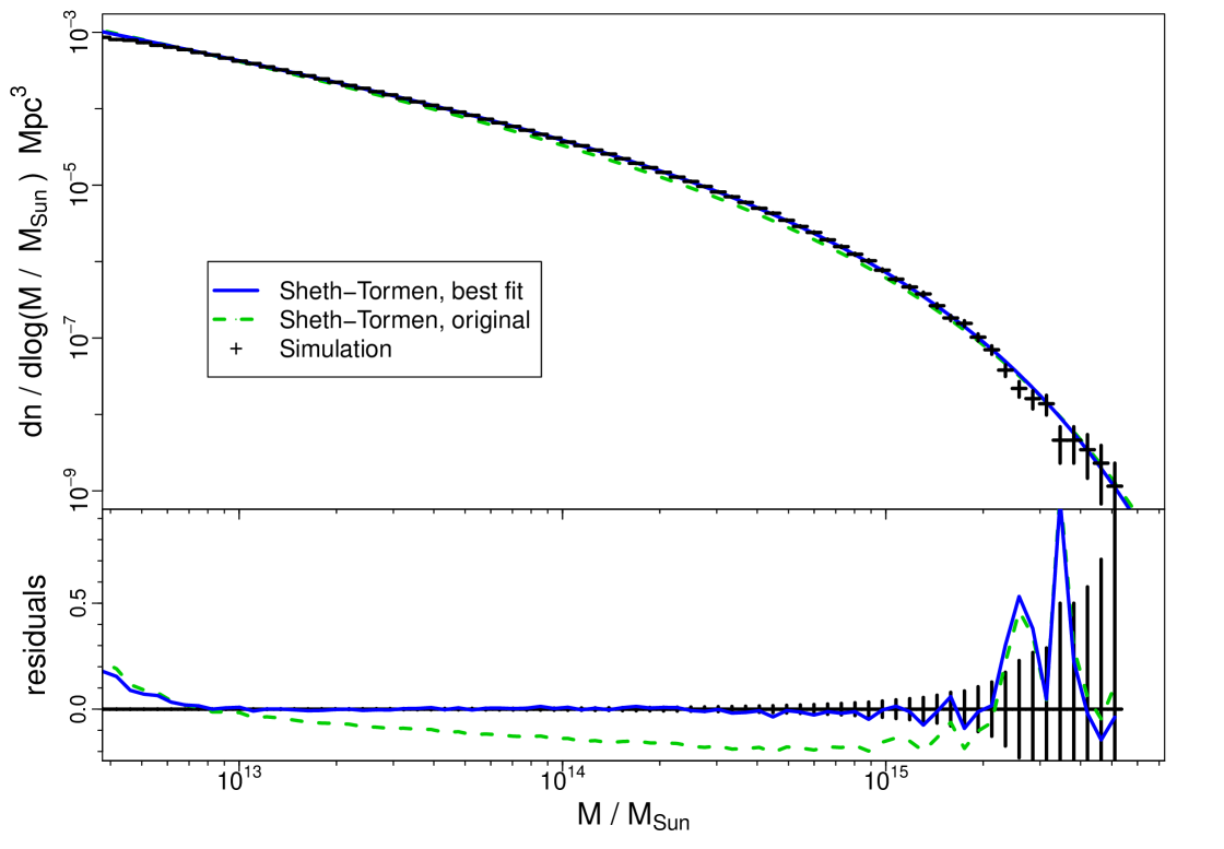
Any discrepancies between our derived Gumbel distribution and the true distribution can be thought of as arising from one of two sources: either inaccuracies in our chosen mass function, or inaccuracies due to the various assumptions made in proceeding from the mass function to $p_{\rm G}$. In order to quantify the respective contributions of each of these two sources, we repeat our calculations with two sets of parameters for the mass function: (i) once taking the parameters used in Sheth & Tormen (1999), $(p,a)=(0.3,0.707)$, and, since the Sheth & Tormen form is its standard parametrisation is known to perform only approximately (e.g. Warren et al., 2006; Jenkins et al., 2001), (ii) once with a best fit for $a$ and $p$ to the simulation’s mass function, leading to $(p,a)=(-0.19,0.777)$. For this latter, we also weight bins by their mass, since it is the high-mass end of the distribution which is of interest to us. Fig. 1 shows both these mass functions along with that measured in the simulation.

(a) $L=100/h$ Mpc; $\gamma=-0.11$

(b) $L=50/h$ Mpc; $\gamma=-0.14$

(c) $L=20/h$ Mpc; $\gamma=-0.11$

(d) $L=8/h$ Mpc; $\gamma=-0.12$

Figure 2: Distribution of largest cluster masses $m_{\rm max}$. The y axis is probability density per log mass. Points are measurements from the simulation with Poisson error bars for each mass bin. The solid blue line is the theoretical result using the best-fit mass function ($p=-0.19,a=0.777$) and full halo clustering. Green dashes have instead the original Sheth-Tormen parameters ($p=0.3,a=0.707$). Not surprisingly, they do not agree as well with the measurement as the solid blue line; red dots have the best-fit values but assume halos are Poisson distributed. The orange dot-dashed line is the Generalised Extreme Value distribution, with parameters calculated as explained in section 2.4 and assuming Poisson statistics. All calculations use spherical patches, with radius $L=100,50,20,8h^{-1}$ Mpc respectively.

3.2 Results

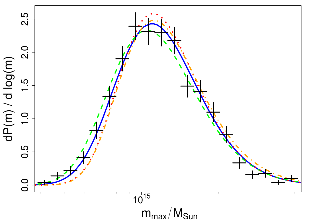
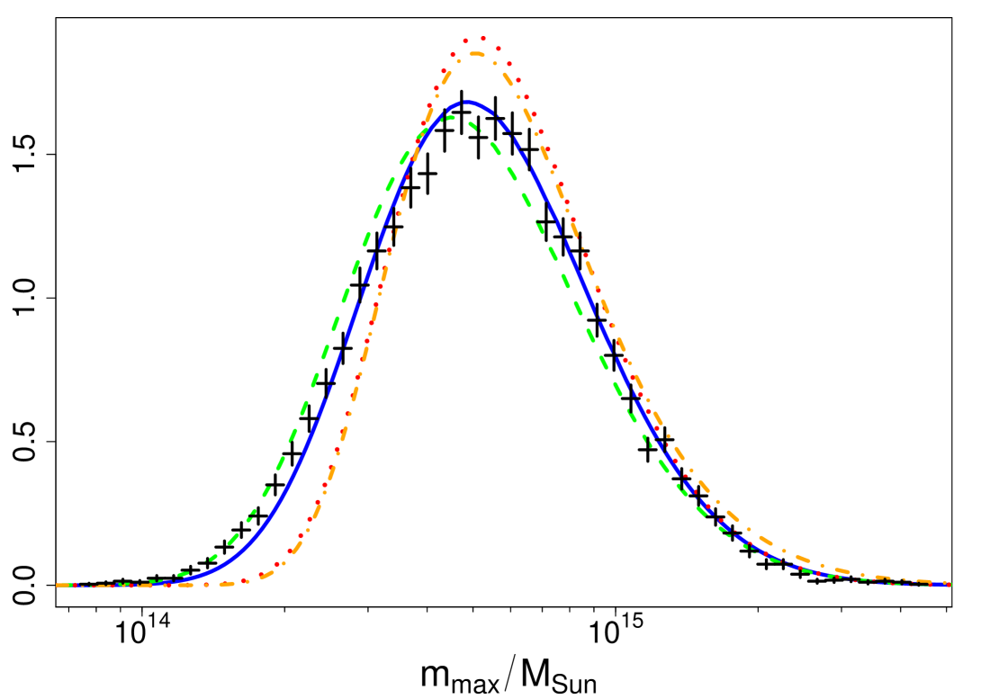
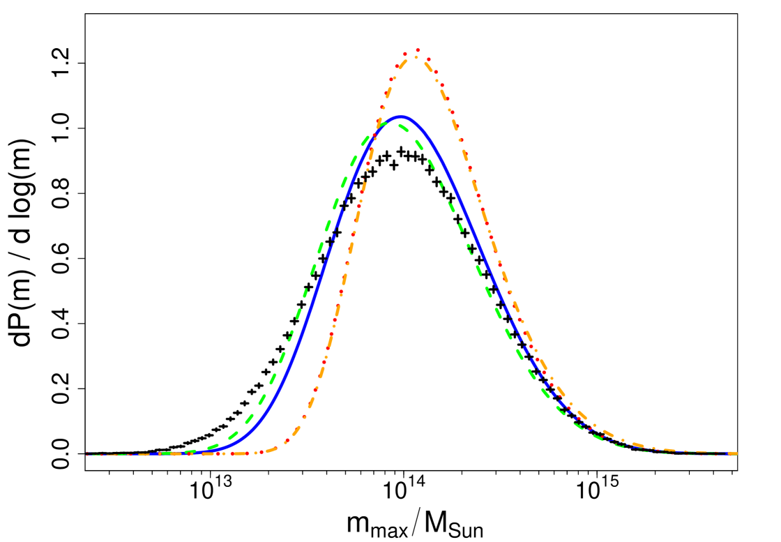
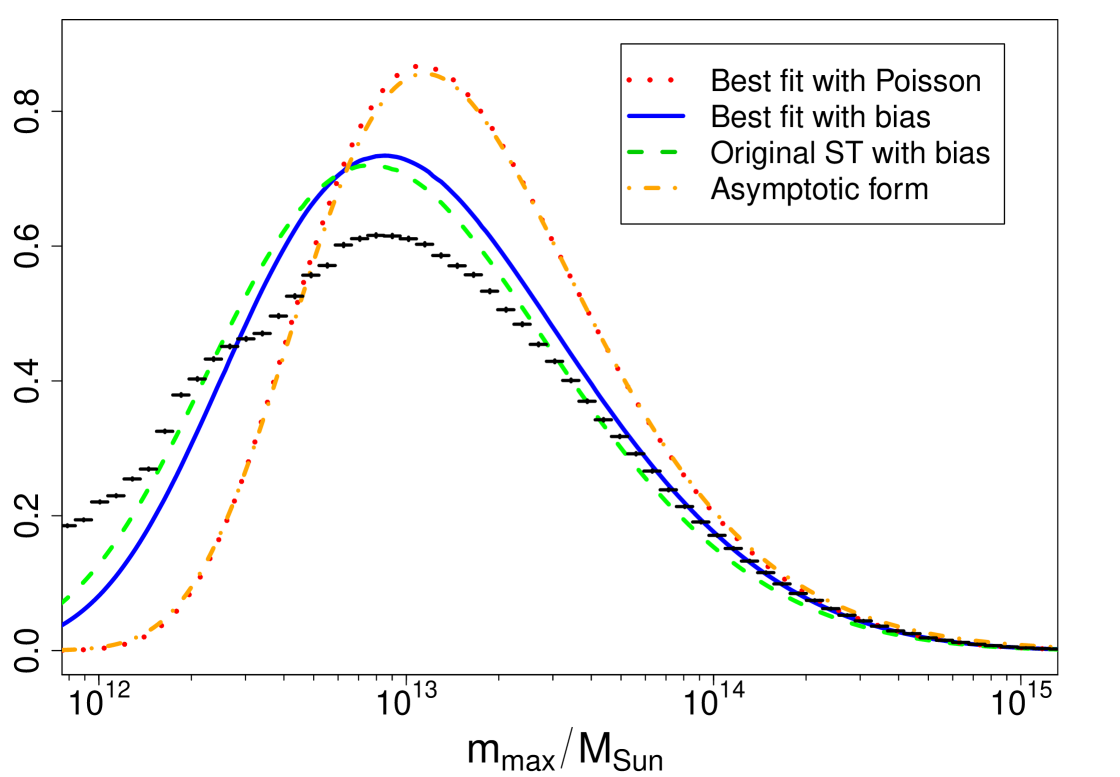
Fig. 2 shows the distribution $p_{\rm G}(m_{\rm max})$ calculated as above, both for Poisson statistics (equation 4, red dots) and incorporating full clustering (equation 7, blue solid lines) using our best-fit mass function. The full clustering calculation is also shown for the original Sheth-Tormen parameters (green dashes). Points show measurements from the Horizon 4$\Pi$ simulation for comparison.

Fitting a Gumbel distribution eq. (1) to the data presented in the four panels of this figure yields a single value of $\gamma$ around -0.21 $\pm^{0.02}_{0.01}$ with reduced $\chi^{2}\leq 1.1$, whereas the analytic prediction presented in section 2.4 gives $-0.14\leq\gamma\leq-0.1$. This lack of agreement has its root in the fact that $\gamma$ is very sensitive to the higher order (skewness and kurtosis) moments of the data distribution around its peak, and these are poorly captured by assuming Poisson statistics, even on $100h^{-1}$ Mpc scales.

However, for a patch (in this case a sphere of radius $L$) of size $L=100h^{-1}$ Mpc, Fig. 2(a) shows that $p_{\rm G}(m_{\rm max})$ measured in the data is not as badly described by Poisson theoretical results as it would have seemed from the value of $\gamma$ alone: we are closing in on the so-called “scale of homogeneity” above which the matter distribution is essentially unclustered. Reducing the patch size to $50h^{-1}$ Mpc (fig. 2(b)) causes the full clustering and Poisson curves to diverge. As expected, only the calculations incorporating clustering remain a good match to the simulation on these smaller scales.

Decreasing $L$ further (fig. 2(c), 2(d)) causes even the calculations including clustering to diverge from the data as our approximations – in particular the expression for the function $\sigma(y)$ in section 2.1 and the condition (14) – fail outside the large-$L$ limit. For instance, we find $R(10^{13}M_{\odot})=3$ Mpc/$h$, and $R(10^{14}M_{\odot})=6.4$ Mpc/$h$ which is a significant fraction of the respective patch sizes of $8$ Mpc/$h$ and $20$ Mpc/$h$. Despite these limitations, the description of the data is still significantly better than that of the Poisson calculation and remains impressive at the high-mass end. This is excellent news as it is this high-mass tail of the distribution which is of interest for assessing the significance of rare events such as surprisingly massive clusters observed in X-ray or redshift surveys. Indeed the lower-mass tail of the distribution for which the prediction fails most significantly lies at masses below $\sim 10^{13}M_{\odot}$, which corresponds to halos containing one to a few galaxies rather than tens or hundreds, and therefore are of limited interest in the search for the most massive cluster.

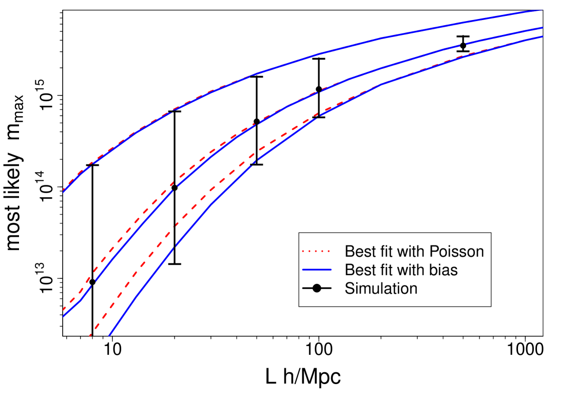
Moreover, note that the position of the peak of the probability distribution function - that is, the most likely value of $\log_{10}m_{\rm max}$ - is fairly accurately predicted by the theory even when the shape of the curve begins to diverge from that of the data. Fig. 3 shows this most likely value, $\log_{10}\hat{m}_{\rm max}$, as a function of $L$ for both theoretical estimates and the simulation data (central line and points in the figure). We also show in this figure the $95\%$ confidence region on $\log_{10}m_{\rm max}$ (upper and lower lines and bars). This too is well fit by the theory, particularly for the upper limit, and we emphasize that this is a crucial test of the theory’s ability to give significance values for observations of specific overly massive clusters.

In addition to the four values of $L$ shown in Fig. 2, Fig. 3 has a final simulation point at $L=500/h$ Mpc. Here the $95\%$ confidence region is poorly fit, because the patch is too large compared to the simulation box to get good statistics. However, the measured value of $\log_{10}m_{\rm max}$ is still in good agreement with the theory.

3.2.1 Senstivity to the mass function

Worthy of note is the close similiarity of the curves for the two sets of parameters in the Sheth-Tormen mass function (solid blue and dashed green lines in Fig. 3). Although the mass functions themselves differ by a relatively large amount compared to the best-fit function’s agreement with the simulation points (Fig. 1, lower panel), this translates to only a modest change in the distribution of $m_{\rm max}$. Similar calculations performed with the mass functions of Tinker et al. (2008) and Jenkins et al. (2001) lead us to conclude that the extreme value distribution is fairly robust to the choice of any reasonable analytic fit to the mass function.

3.2.2 Redshift variation

While the above calculations use patch sizes $L$ small enough that the redshift evolution within the patch is negligible, it is also interesting to calculate $m_{\rm max}$ for a larger region with significant $\Delta z$. As noted in section 2.1, redshift variation can be taken into account by a weighted spatial average provided the Poisson approximation holds, which is the case for such large patches. In particular, averaging the number density of halos over the range $z=0$ to $\infty$ gives a value for the expected largest mass cluster in the entire observable universe.

We performed this calculation assuming Poisson statistics, and found $m_{\rm max}=4.6\pm^{1.2}_{0.6}\times 10^{15}M_{\odot}$ at the $1-\sigma$ confidence level. We note that this is in fair agreement with the similar calculation performed by Holz & Perlmutter (2010), who obtained $m_{\rm max}=3.8\pm^{0.6}_{0.5}\times 10^{15}$ using a WMAP7 cosmology and the mass function of Tinker et al. (2008).

Figure 3: The most likely value of $\log_{10}m_{\rm max}$ (middle line and points) and the $95\%$ confidence limits (upper and lower line and bars). Dashed red and solid blue lines are analytic results for the Poisson limit and full clustering calculations respectively, and points are simulation values for $L$ corresponding to the four panels of fig. 2 plus $L=500/h$ Mpc.

4 Conclusion and Discussion

We have presented an analytic prediction of the the probability distribution of $m_{\rm max}$, the most massive dark matter halo/galaxy cluster in a specified region of the universe, making use of the counts-in-cells formalism. Our calculation, valid for Gaussian initial conditions, is numerically consistent with that proposed by Holz & Perlmutter (2010) when performed assuming such massive halos are Poisson distributed spatially. However, the work presented in this paper improves on the calculation performed by these authors in two aspects: (i) our results are given in a fully explicit analytic form and (ii) they include the contribution of clustering of halos.

We also compared our analytic predictions to measurements from a large (2000$h^{-1}$ Mpc on a side) and well resolved (particle mass $7.7h^{-1}\times 10^{9}$ M_⊙) cosmological $N$-body simulation at zero redshift. We achieve remarkable agreement with the simulation in the area of parameter space in which our formalism is expected to be valid, namely patch radii above a few tens of $h^{-1}$ Mpc. More surprisingly, even outside this range of scales the high-mass tail of the distribution is well fit by our ”fully clustered” theoretical estimate, as is the most likely value of $\log_{10}m_{\rm max}$.

This unexpected success over a wide range of scales warrants the application of the formalism to quantify the statistical significance of individual clusters observed in surveys. By applying our method to a patch of shape, size and redshift equivalent to a real survey we can obtain the Gumbel distribution and hence a likelihood for the observed value of $m_{\rm max}$. Moreover, we are quite confident that our method can be extended to non-standard cosmologies such as those including initial non-Gaussianities. It could therefore provide a measure of the evidence for such cosmologies from existing surveys of the most massive clusters as advocated in Cayón et al. (2010). We plan to tackle this exciting prospect in the very near future.

In addition to the full likelihood curve of $m_{\rm max}$ we are able, via the analytic Generalised Extreme Value formalism, to produce a summary of the distribution in the form of the three parameters $a$, $b$ and $\gamma$. The latter in particular has been proposed previously as a statistic for use in model comparison (e.g. Mikelsons et al., 2009). Although the work described in this paper uses a single cosmology and power spectrum and produces a roughly constant value of $\gamma$, the results of Colombi et al. (2010) suggest that $\gamma$ should be quite sensitive to the shape of the power spectrum. If the effect on $\gamma$ of the clustering can be fully quantified, we therefore expect to be able to use it as a statistic for direct comparison of models with observation. Likewise $a$, which is closely related to the peak $m_{0}$ of the distribution, may prove a useful statistic since we have demonstrated that it is well predicted by our theory.

5 Acknowledgements

The authors are grateful to an anonymous reviewer whose comments led to improvements in this paper.

JD’s research is supported by the Oxford Martin School, Adrian Beecroft and STFC.

CP acknowledges support from a Leverhulme visiting professorship at the Astrophysics department of the University of Oxford.

References

- Antal et al. [2009] Antal T., Sylos Labini F., Vasilyev N. L., Baryshev Y. V., 2009, Europhysics Letters, 88, 59001
- Balian & Schaeffer [1989] Balian R., Schaeffer R., 1989, A&A, 220, 1
- Bernardeau & Schaeffer [1999] Bernardeau F., Schaeffer R., 1999, A&A, 349, 697
- Bhavsar & Barrow [1985] Bhavsar S. P., Barrow J. D., 1985, MNRAS, 213, 857
- Cayón et al. [2010] Cayón L., Gordon C., Silk J., 2010, arXiv:1006.1950
- Coles [1988] Coles P., 1988, MNRAS, 231, 125
- Colombi et al. [2010] Colombi S., Davis O., Devriendt J. E. G., Silk J., 2010, submitted to MNRAS
- Davis et al. [1985] Davis M., Efstathiou G., Frenk C. S., White S. D. M., 1985, ApJ, 292, 371
- Gumbel [1958] Gumbel E., 1958, Statistics of extremes. Columbia University Press
- Holz & Perlmutter [2010] Holz D. E., Perlmutter S., 2010, arXiv:1004.5349
- Jenkins et al. [2001] Jenkins A., Frenk C. S., White e. a., 2001, MNRAS, 321, 372
- Mantz et al. [2008] Mantz A., Allen S. W., Ebeling H., Rapetti D., 2008, MNRAS, 387, 1179
- Mantz et al. [2010] Mantz A., Allen S. W., Rapetti D., 2010, MNRAS, 406, 1805
- Mantz et al. [2010] Mantz A., Allen S. W., Rapetti D., Ebeling H., 2010, MNRAS, 406, 1759
- Matsubara et al. [1997] Matsubara T., Suto Y., Szapudi I., 1997, ApJ, 491, L1+
- Mikelsons et al. [2009] Mikelsons G., Silk J., Zuntz J., 2009, MNRAS, 400, 898
- Mo et al. [1996] Mo H. J., Jing Y. P., White S. D. M., 1996, MNRAS, 282, 1096
- Mo & White [1996] Mo H. J., White S. D. M., 1996, MNRAS, 282, 347
- Press & Schechter [1974] Press W. H., Schechter P., 1974, ApJ, 187, 425
- Rapetti et al. [2010] Rapetti D., Allen S. W., Mantz A., Ebeling H., 2010, MNRAS, 406, 1796
- Sheth & Tormen [1999] Sheth R. K., Tormen G., 1999, MNRAS, 308, 119
- Spergel et al. [2007] Spergel D. N., Bean R., Doré O., et al. 2007, ApJS, 170, 377
- Szapudi & Szalay [1993] Szapudi I., Szalay A. S., 1993, ApJ, 408, 43
- Teyssier [2002] Teyssier R., 2002, A&A, 385, 337
- Teyssier et al. [2009] Teyssier R., Pires S., Prunet S., et al. 2009, A&A, 497, 335
- Tinker et al. [2008] Tinker J., Kravtsov A. V., Klypin A., Abazajian K., Warren M., Yepes G., Gottlöber S., Holz D. E., 2008, ApJ, 688, 709
- Tinker et al. [2010] Tinker J. L., Robertson B. E., Kravtsov A. V., Klypin A., Warren M. S., Yepes G., Gottlober S., 2010, ArXiv e-prints
- Warren et al. [2006] Warren M. S., Abazajian K., Holz D. E., Teodoro L., 2006, ApJ, 646, 881
- Yamila Yaryura et al. [2010] Yamila Yaryura C., Baugh C. M., Angulo R. E., 2010, ArXiv e-prints
- Zeldovich et al. [1982] Zeldovich I. B., Einasto J., Shandarin S. F., 1982, Nature, 300, 407