A simple description of jet cross-section ratios

Abstract

We compute the ratio of the inclusive jet cross-sections obtained with the same jet algorithm at two different values of the jet radius. We perform a computation of that observable at NLO (${\cal{O}}\left(\alpha_{s}^{2}\right)$) in perturbative QCD and compute non-perturbative corrections from soft-gluon emission. We discuss predictions for RHIC and the LHC.

Introduction

In this letter, we are interested in computing the ratio of the inclusive jet cross-section computed with the same jet algorithm at two different values of $R$:

$${\cal R}(p_{t};R_{1},R_{2})=\frac{\frac{d\sigma}{dp_{t}}(R=R_{1})}{\frac{d\sigma}{dp_{t}}(R=R_{2})}.$$ (1)

Our main objective is to show that the minimal effort required to get a reliable prediction for ${\cal R}$ is to include ${\cal{O}}\left(\alpha_{s}^{2}\right)$ perturbative correction as well as (universal) non-perturbative power corrections.

We shall first discuss the perturbative computation of ${\cal R}$. This is interesting per se since, as we will see below, instead of computing naively the ratio of the cross-sections computed at NLO, which would formally correspond to a computation of ${\cal R}$ up to ${\cal{O}}\left(\alpha_{s}\right)$, it is actually possible to obtain the ${\cal{O}}\left(\alpha_{s}^{2}\right)$ corrections [1].

Since jets are basic observables at the LHC, and both ATLAS and CMS plan to use the anti-$k_{t}$ algorithm [3] with two different radii ($R=0.4$ and $0.6$ for ATLAS, $R=0.5$ and $0.7$ for CMS), they could in principle measure the ratio. Compared to the measurement of the inclusive jet cross-section, the ratio would not have the uncertainty on the luminosity measurement and would probably be less sensitive to the jet energy scale. Below, we shall compare our NLO QCD predictions with and without hadronisation corrections to the ATLAS recent measurements [4] and make predictions for the cross-section ratio.

Another situation in which the cross-section ratio is an interesting observable is at RHIC where it can be measured both in proton-proton and heavy-ion collisions. Due to the interaction with the hot medium produced in heavy-ion collisions, one expects the jet to loose energy and to be broadened. That would directly translate into a decrease of the cross-section ratio (see e.g. [5] for a computation with and without medium effects at ${\cal{O}}\left(\alpha_{s}\right)$ in QCD). Here we shall show that, for the $pp$ reference measurement, the next order and hadronisation bring large corrections.

Perturbative expansion

Let us start with a perturbative QCD computation of the cross-section ratio. Naively, since inclusive jet cross-sections are known up to NLO accuracy (${\cal{O}}\left(\alpha_{s}^{3}\right)$), one would use

$${\cal R}(p_{t};R_{1},R_{2})=\frac{\sigma^{\mathrm{NLO}}(p_{t};R_{1})}{\sigma^{\mathrm{NLO}}(p_{t};R_{2})},$$ (2)

which is formally an ${\cal{O}}\left(\alpha_{s}\right)$ computation of ${\cal R}$.

The interesting point is that, by making the perturbative expansion explicit, ${\cal R}$ can actually be computed up to ${\cal{O}}\left(\alpha_{s}^{2}\right)$. To see this, consider the perturbative expansion of the jet cross-section:

$$\sigma(p_{t};R)=\alpha_{s}^{2}\sigma^{(2)}(p_{t})+\alpha_{s}^{(3)}\sigma^{3}(p_{t};R)+\alpha_{s}^{4}\sigma^{(4)}(p_{t};R)+{\cal{O}}\left(\alpha_{s}^{5}\right),$$

where we have taken into account the fact that the leading-order contribution does not depend on $R$. The contribution $\sigma^{(n)}(p_{t};R)$ at a given order $\alpha_{s}^{n}$ receives contributions from tree diagrams with $n$ particles in the final-state, up to $(n-2)$-loop diagrams with 2 particles in the final state. Denoting by $\sigma^{(n,p)}(p_{t};R)$ the $p$-loop contribution to $\sigma^{(n)}(p_{t};R)$, we have

$$\sigma(p_{t};R) = \alpha_{s}^{2}\sigma^{(2,0)}(p_{t})+\alpha_{s}^{3}[\sigma^{(3,0)}(p_{t};R)+\sigma^{(3,1)}(p_{t})]$$ (3)

$$+ \alpha_{s}^{4}[\sigma^{(4,0)}(p_{t};R)+\sigma^{(4,1)}(p_{t};R)+\sigma^{(4,2)}(p_{t})]+{\cal{O}}\left(\alpha_{s}^{5}\right),$$

where we have again used the fact that the contributions with only 2 particles in the final state do not depend on the jet radius $R$.

If we use (3) to expand the ratio ${\cal R}(R_{1},R_{2})$ in series of $\alpha_{s}$, we obtain, up to corrections of order $\alpha_{s}^{3}$,

$${\cal R}(p_{t};R_{1},R_{2}) = 1+\alpha_{s}\frac{\Delta\sigma^{(3,0)}(p_{t};R_{1},R_{2})}{\sigma^{(2)}(p_{t})}$$

$$+ \alpha_{s}^{2}\frac{\Delta\sigma^{(4,0)}(p_{t};R_{1},R_{2})+\Delta\sigma^{(3,1)}(p_{t};R_{1},R_{2})}{\sigma^{(2)}(p_{t})}-\alpha_{s}^{2}\frac{\sigma^{(3)}(p_{t};R_{2})\Delta\sigma^{(3,0)}(p_{t};R_{1},R_{2})}{[\sigma^{(2)}(p_{t})]^{2}},$$

with $\Delta\sigma^{(n,p)}(p_{t};R_{1},R_{2})=\sigma^{(n,p)}(p_{t};R_{1})-\sigma^{(n,p)}(p_{t};R_{2})$.

The remarkable fact, that allows for the computation to be performed at ${\cal{O}}\left(\alpha_{s}^{2}\right)$, is that the two-loop contribution to the NNLO jet-cross-section, that prevents one from obtaining a NNLO computation of the inclusive jet cross-section (e.g. using NLOJet [6]), does not appear in the computation of the cross-section ratio.

In what follows, the LO ratio will refer to (Perturbative expansion) with the two first terms kept — the ${\cal{O}}\left(\alpha_{s}\right)$ expansion, i.e. the first non-trivial order —, while the NLO ratio will also incorporate the ${\cal{O}}\left(\alpha_{s}^{2}\right)$ corrections in (Perturbative expansion).

Before proceeding with the discussion about non-perturbative effects, it is interesting to comment a bit on eq. (Perturbative expansion). In the collinear limit, the NLO (resp. NNLO) correction to the cross-section will be proportional to $\alpha_{s}\log(1/R)$ (resp. $\alpha_{s}^{2}\log^{2}(1/R)$), which would be the dominant correction at small jet radius. In the computation of the ratio, the ${\cal{O}}\left(\alpha_{s}\right)$ term only involves the cross-section difference and will thus be proportional to $\log(R_{1}/R_{2})$ while the next order will involve $\log(R_{1}/R_{2})\log(1/R_{2})$. This means that for $R_{1}\sim R_{2}\ll 1$, the collinear contribution will mostly appear from NLO onwards and we may thus expect large NLO corrections.

Non-perturbative corrections

As we shall see later when making explicit computations of the ratio ${\cal R}$, for small values of $R$, hadronisation corrections may have a significant impact on the jet cross-section and thus on ${\cal R}$. One could in principle rely on Pythia [7] or Herwig [8] (or, better, a combination of both) in order to estimate the correction factor one has to apply to go from a parton-level cross-section to a hadron-level cross-section, i.e. to estimate hadronisation corrections. Keeping in mind that we want to provide as simple a description of the cross-section ratio as we can, we shall instead give an analytic estimate of the hadronisation corrections. In [1], hadronisation correction are computed from soft-gluon emission and the authors obtain that the effect of hadronisation is to shift the $p_{t}$ of the jet by an average amount

$$\left\langle\delta p_{t}\right\rangle_{\rm hadr}=\frac{-2C_{R}}{R}\frac{2M}{\pi}{\cal A}(\mu_{I}).$$ (5)

In that expression, $C_{R}$ if the Casimir factor which should be $C_{F}$ for quark jets and $C_{A}$ for gluon jets, $M$ is the Milan factor that depends on the jet algorithm — it is universal [9], $M\approx 1.49$, for the anti-$k_{t}$ algorithm while, for the $k_{t}$ algorithm, one finds [10] $M\approx 1.01$ —, and ${\cal A}(\mu_{I})$ carries all the non-perturbative dependence. The latter can be rewritten as

$${\cal A}(\mu_{I})=\frac{\mu_{I}}{\pi}\left[\alpha_{0}(\mu_{I})-\alpha_{s}(p_{t})-\frac{\beta_{0}}{2\pi}\left(\log\left(\frac{p_{t}}{\mu_{I}}\right)+\frac{K}{\beta_{0}}+1\right)\alpha_{s}^{2}(p_{t})\right],$$ (6)

where the average coupling in the infrared region $\alpha_{0}(\mu_{I})=(1/\mu_{I})\int_{0}^{\mu_{I}}\alpha_{s}(k_{t})dk_{t}$ is frequently encountered in event-shape studies (see e.g. [11]), $\beta_{0}=(11C_{A}-2n_{f})/3$ and $K=C_{A}\left(\frac{67}{16}-\frac{\pi^{2}}{6}\right)-\frac{5}{9}n_{f}$.

Including the hadronisation corrections to the perturbative cross-section can then be done using

$$K_{\rm hadr}(p_{t};R)=\frac{\sigma(p_{t};R)}{\sigma_{\rm pQCD}(p_{t};R)}\approx\frac{\sigma_{\rm pQCD}(p_{t}-\left\langle\delta p_{t}\right\rangle_{\rm hadr};R)}{\sigma_{\rm pQCD}(p_{t};R)}\approx\frac{\sigma_{\rm LO}(p_{t}-\left\langle\delta p_{t}\right\rangle_{\rm hadr};R)}{\sigma_{\rm LO}(p_{t};R)}.$$ (7)

For the first equality, we have neglected the dispersion in $\delta p_{t}$ (i.e. assumed that the shift was always the average one) which would correspond to higher power corrections that are not as well controlled from LEP data. Approximating the full perturbative cross-section by the leading-order expression in the second equality is motivated by the fact that the computation of hadronisation corrections from soft-gluon emission is done for the underlying $2\to 2$ scattering i.e. from the leading-order process.

Finally, the cross-section ratio after taking into account the hadronisation corrections is

$${\cal R}(p_{t};R_{1},R_{2})=\frac{K_{\rm hadr}(p_{t};R_{1})}{K_{\rm hadr}(p_{t};R_{2})}{\cal R}_{\rm pQCD}(p_{t};R_{1},R_{2}),$$ (8)

with ${\cal R}_{\rm pQCD}(p_{t};R_{1},R_{2})$ computed from eq. (Perturbative expansion).

Because of the $1/R$ behaviour of (5), we may also expect sizeable effects from the non-perturbative corrections at small $R$. Note however that the factor of the $1/R$ term is rather small ($2C_{F}{\cal A}(\mu_{I})\approx 0.5\,\mathrm{GeV}$), compared to the corresponding QCD corrections that would typically scale like $\alpha_{s}p_{t}$ and so dominate at moderate $R$ and $p_{t}$.

Comparison with experiments

In the following lines, we briefly discuss the perturbative computation of ${\cal R}$ and the hadronisation corrections at two different energies: RHIC ($\sqrt{s}=200\,\mathrm{GeV}$) and the LHC ($\sqrt{s}=7\,\mathrm{TeV}$).

As far as the perturbative part of the computation is concerned, we have used NLOJet (v4.1.2) [6] for the computation of the different pieces in (Perturbative expansion). We have considered the CTEQ6.6 NLO PDF set [12] as well as the MSTW08 NLO and NNLO sets [13] though, for brevity, we shall only show the CTEQ6.6 results in what follows. The scale uncertainties have been obtained by varying independently the renormalisation and factorisation scales from $p_{t,{\rm jet}}$ to $p_{t,{\rm jet}}/2$ and $2p_{t,{\rm jet}}$.

Figure 1: QCD predictions for the ratio ${\cal R}(p_{t};0.2,0.4)$ at RHIC ($\sqrt{s}=200\,\mathrm{GeV}$) for the anti-$k_{t}$ (left) and $k_{t}$ (right) jet algorithms. On the top panel, the solid lines correspond, from top to bottom, to the LO QCD computation (green), to the NLO QCD ratio (red) and to the NLO QCD computation including hadronisation effects (blue). The uncertainties due to the scale choice and, when relevant, hadronisation are shown as shaded bands on the top panel and the relative scale uncertainty is plotted on the bottom panel. For comparison, we have also plotted in dashed lines the parton-level (red) and hadron-level (blue) predictions from Pythia.

To compute the hadronisation corrections, the only parameter we need is $\alpha_{0}$. As already mentioned, this can be extracted [11] from event-shape distributions at LEP and we shall use the value $\alpha_{0}(\mu_{I})=0.503$ with $\mu_{I}=2\,\mathrm{GeV}$, obtained from JADE data [14]. The uncertainty on the hadronisation corrections will be estimated by varying the Milan factor ($M=1.49$ for the anti-$k_{t}$ algorithm and $M=1.01$ for $k_{t}$) by the standard 20%.

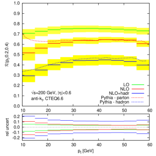
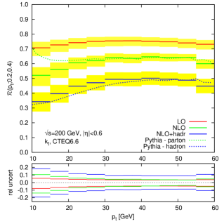
Let us start by discussing the case of RHIC, where STAR is planning to measure [15] the ratio ${\cal R}(p_{t};0.2,0.4)$ for both the $k_{t}$ [16] and anti-$k_{t}$ [3] algorithms. Though the ratio will be measured in proton-proton and gold-gold collisions with the ultimate goal to see jet-broadening effects due to interaction with the hot medium produced in heavy-ion collisions, we just focus on the $pp$ case here. The result is presented in Fig. 1 for both algorithms. The first message is that NLO corrections to ${\cal R}$ are substantial ($\sim 0.1-0.15$) and, probably as a consequence, the scale uncertainty does not decreases when going from LO to NLO. Though they are strictly the same only at LO, the $k_{t}$ and anti-$k_{t}$ algorithms show a very similar cross-section ratio also at NLO. Then, as a consequence of the choice of rather small values of $R$, hadronisation effects are also sizeable ($\sim 0.15-0.2$). In this case, since the Milan factor is a bit larger for the anti-$k_{t}$ algorithm than for $k_{t}$, the final ratio tends to be a bit larger for the $k_{t}$ algorithm. Finally, Fig. 1 shows that the NLO pQCD computation of $\cal{R}$ is in good agreement with what is obtained from Pythia (v6.4) at parton-level (i.e. including parton shower from initial and final-state radiation), and our final prediction, including non-perturbative corrections is also in good agreement with what Pythia predicts when hadronisation is included.

Figure 2: Left: comparison of our inclusive jet cross-section computations with the ATLAS measurements. The ratio between the experimental values and the theory predictions (NLO QCD including non-perturbative effects) is plotted; the yellow band represents the uncertainty on the theoretical prediction and the cyan band corresponds to the NLO QCD prediction without hadronisation corrections. Right: predictions for the ratio ${\cal R}(p_{t};0.4,0.6)$ for the anti-$kt$ algorithm at ,from top to bottom, LO, NLO, NLO with hadronisation corrections. See Fig. 1 for conventions.

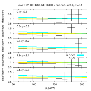
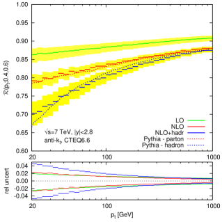
We now turn to the case of measurements at the LHC and, more precisely, to the jet cross-section measured very recently at $\sqrt{s}=7\,\mathrm{TeV}$ by the ATLAS collaboration [4]. On Fig. 2 we have plotted our predictions both for the jet cross-section (anti-$k_{t}$ algorithm with $R=0.4$) and the cross-section ratio ${\cal R}(p_{t};R_{1}=0.4,R_{2}=0.6)$. The jet cross-section is compared to the ATLAS measurements and we see that, though the pure NLO QCD prediction (cyan band) describes the data nicely, the inclusion of the non-perturbative power corrections improves the description. Note also that the non-perturbative corrections obtained in our approach are compatible with the numbers obtained from Pythia and Herwig and quoted by ATLAS. If we now consider the cross-section ratio, see the right plot on Fig. 2, we basically recover the main features already discussed in the case of RHIC. However, both the NLO QCD corrections and the hadronisation corrections are reduced compared to what we observed at RHIC. This is even more true for the non-perturbative corrections at large $p_{t}$ which become very small. This is likely due to two effects: first, the considered radii are larger, reducing the effect of the collinear divergence in the NLO QCD computation as well as the hadronisation corrections that behave like $1/R$. Then, the inclusive jet cross-section is much less steep at the LHC than at RHIC and thus a common $p_{t}$ shift would have a larger impact at RHIC.

Conclusions

To summarise, we have discussed in this letter the minimal ingredients needed to get a reliable calculation of the ratio ${\cal R}(p_{t};R_{1},R_{2})$ of the $p_{t}$-dependent inclusive jet cross-section computed with the same jet algorithm at two different values, $R_{1}$ and $R_{2}$, of the jet radius.

We have seen that by making an explicitly expansion in powers of $\alpha_{s}$, we can compute ${\cal R}$ perturbatively at ${\cal{O}}\left(\alpha_{s}^{2}\right)$, the NLO accuracy for that observable, that is one order higher than what we would naively expect from the direct ratio of the cross-sections. The explicit computation of ${\cal R}$ at NLO can be done e.g. using the NLOJet++ event generator. Note that using techniques of [17] would allow us to obtain an approximate NNLO calculation and further test the convergence of the perturbative series.

Then, we have estimated the non-perturbative corrections to the ratio. They are based on universal power corrections and the only free parameter, $\alpha_{0}$, can be estimated from fits to event-shape measurements at LEP.

Finally, we have seen that, in practice, both the ${\cal{O}}\left(\alpha_{s}^{2}\right)$ terms and the non-perturbative effects are numerically sizeable, except for the hadronisation correction at large $p_{t}$. In the case of the recent jet measurements done by ATLAS, it would be interesting to see if the computation of the ratio could benefit from reduced uncertainties compared to the jet cross-section itself.

In the case of RHIC, the NLO and hadronisation corrections are even larger. It is important to keep that in mind when performing the same computation for heavy-ion collisions, in the presence of the medium: the one-gluon-emission approximation is likely to be insufficient. One has to include the next-order corrections as well as non-perturbative effects.

References

- [1] M. Dasgupta, L. Magnea and G. P. Salam, JHEP 0802 (2008) 055 [arXiv:0712.3014].
- [2] H. Abramowicz et al. [ZEUS Collaboration], Phys. Lett. B 691 (2010) 127 [arXiv:1003.2923].
- [3] M. Cacciari, G. P. Salam and G. Soyez, JHEP 0804 (2008) 063 [arXiv:0802.1189].
- [4] ATLAS Collaboration, CERN-PH-EP-2010-034, arXiv:1009.5908.
- [5] I. Vitev and B. W. Zhang, Phys. Rev. Lett. 104 (2010) 132001 [arXiv:0910.1090].
- [6] Z. Nagy, Phys. Rev. Lett. 88 (2002) 122003 [arXiv:hep-ph/0110315]; Phys. Rev. D 68 (2003) 094002 [arXiv:hep-ph/0307268].
- [7] T. Sjostrand, S. Mrenna and P. Skands, JHEP05 (2006) 026 [arXiv:hep-ph/0603175].
- [8] G. Corcella et al., arXiv:hep-ph/0210213.
- [9] Y. L. Dokshitzer, A. Lucenti, G. Marchesini and G. P. Salam, JHEP 9805 (1998) 003 [arXiv:hep-ph/9802381].
- [10] M. Dasgupta and Y. Delenda, JHEP 0907 (2009) 004 [arXiv:0903.2187].
- [11] Y. L. Dokshitzer and B. R. Webber, Phys. Lett. B 352 (1995) 451 [arXiv:hep-ph/9504219]. M. Dasgupta and G. P. Salam, J. Phys. G 30 (2004) R143 [arXiv:hep-ph/0312283].
- [12] P. M. Nadolsky et al., Phys. Rev. D 78 (2008) 013004 [arXiv:0802.0007].
- [13] A. D. Martin, W. J. Stirling, R. S. Thorne and G. Watt, Eur. Phys. J. C 63 (2009) 189 [arXiv:0901.0002].
- [14] P. A. Movilla Fernandez, arXiv:hep-ex/0209022.
- [15] M. Ploskon [STAR Collaboration], Nucl. Phys. A 830 (2009) 255C [arXiv:0908.1799].
- [16] S. Catani, Y. L. Dokshitzer, M. H. Seymour and B. R. Webber, Nucl. Phys. B 406 (1993) 187 and refs. therein; S. D. Ellis and D. E. Soper, Phys. Rev. D 48 (1993) 3160 [arXiv:hep-ph/9305266].
- [17] M. Rubin, G. P. Salam and S. Sapeta, JHEP 1009 (2010) 084 [arXiv:1006.2144 [hep-ph]].