Coupling between QPOs and broadband noise components in GRS 1915+105
Abstract
We explore the use of the bispectrum for understanding quasiperiodic oscillations. The bispectrum is a statistic which probes the relations between the relative phases of the Fourier spectrum at different frequencies. The use of the bispectrum allows us to break the degeneracies between different models for time series which produce identical power spectra. We look at data from several observations of GRS 1915+105 when the source shows strong quasi-periodic oscillations and strong broadband noise components in its power spectrum. We show that, despite strong similarities in the power spectrum, the bispectra can differ strongly. In all cases, there are frequency ranges where the bicoherence, a measure of nonlinearity, is strong for frequencies involving the frequency of the quasi-periodic oscillations, indicating that the quasi-periodic oscillations are coupled to the noise components, rather than being generated independently. We compare the bicoherences from the data to simple models, finding some qualitative similarities.
keywords:
accretion, accretion discs – methods: statistical – X-rays:binaries – stars:winds,outflows – stars:binaries:close1 Introduction
Recent studies of the variability properties of accreting black holes and neutron stars have shown that these systems’ Fourier power spectra in certain spectral states are well-described by a sum of many Lorentzian components (see e.g. Olive et al. 1998; Nowak 2000; Belloni, Psaltis & van der Klis 2002; van Straaten et al. 2002; Pottschmidt et al. 2003). Essentially the same components seem to appear in nearly all sources, and at nearly all luminosities, and their frequencies tend to be well correlated with one another and with the source spectral states (Wijnands & van der Klis 1999; Psaltis, Belloni & van der Klis 1999). This phenomenology suggests that there may be a single origin for most of the variability features in the power spectra of accreting black holes and neutron stars. Similar correlations in frequencies between the different components seem to apply even to accreting white dwarfs (e.g. Mauche 2002; Warner, Woudt & Pretorius 2003).
Coupling between different components in the power spectrum has been suggested in many theoretical contexts. In a shot noise model (e.g. Terrell 1972), variability components on the timescale of the shot will be correlated with one another, resulting in, e.g. fast rise exponential decay or exponential rise, fast decay profiles, but there should be no coupling on timescales longer than those of the shots. More sophisticated models of variability, for example, self-organized criticality (e.g. Takeuchi, Mineshige & Negoro 1995; Takeuchi & Mineshige 1997), predict correlations between the arrival times and/or intensities of the shots. Other related “reservoir” models (e.g. Merloni & Fabian 2001; Maccarone & Coppi 2002; Malzac, Merloni & Fabian 2004), where the accretion disk and/or the relativistic jet taps an energy supply effectively enough to reduce the available energy for future emission also predict variability correlated over many frequencies. Resonance models for producing quasi-periodic oscillations should also clearly produce non-linear variability (e.g. Psaltis & Norman 2001; Abramowicz & Kluzniak 2001; Schnittman & Bertschinger 2003; Maccarone & Schnittman 2005), while non-resonant models for producing the same QPOs (e.g. Chen & Taam 1992,1995; Rezzolla et al. 2003; Giannios & Spruit 2004) could, but need not show coupling between the different frequencies. Propagation models, where disturbances move through an accretion disc, also should produce non-linear coupling of variability components, as the variability properties are modified at each annulus (Lyubarskii 1997).
A key to verifying and understanding this possible unified origin for variability is to go beyond the simple power spectrum and begin studying their non-linear variability. The first attempts at this failed to detect signatures of non-linearity, with the methods including the time skewness (Priedhorsky et al. 1978) and searches for a low dimensional chaotic attractor (Lochner, Swank & Szymkowiak 1989). On the other hand, more recent work with better light curves did establish that the light curves of Cygnus X-1 are not time reversible (Timmer et al. 2000; Maccarone & Coppi 2002), that there exists a correlation between rms amplitude and flux of a source that is inconsistent with pure shot noise models (Uttley & McHardy 2001), that there is coupling between variability components on all observable time scales (Maccarone & Coppi 2002), and that in some cases, there is a low dimensional chaotic attractor after all (Misra et al. 2004), and the observed light curves may be described by a Lorenz system (Misra et al. 2006). With this in mind, we now approach looking at the properties of the coupling between quasi-periodic components and noise components in GRS 1915+105, a bright Galactic X-ray binary with an accreting black hole which has been the subject of several long observations with the Rossi X-ray Timing Explorer (RXTE).
We treat this work as a pilot study – the first attempt to apply the bispectrum to astronomical data with strong quasi-periodic oscillations. As such, we aim to illustrate the power of the technique by showing data and simple models that can give very similar power spectra, and very different bicoherences, but consider it beyond the scope of the work to try to fit models to the data precisely. We present computations of the bicoherence for several observations of GRS 1915+105, discuss the meaning of the bicoherence, and present a few toy models for the bicoherence which we compare with the data.
2 Data Used
For this pilot study, we present the results from three representative observations of GRS 1915+105; our goals in this paper are not to make a complete characterisation of the bicoherence properties of all sources in all states, but rather to demonstrate of the utility of the technique for identifying phenomenological differences between apparently rather similar lightcurves with rather similar power spectra, and to show a few theoretical models that produce bicoherences similar to some of the observations. All these data are from variability class in the classification scheme of Belloni et al. (2000). In this class, GRS 1915+105 stays steadily in state C, its “low/hard” state – the “hard very high state” in the nomenclature of Fender & Belloni (2004), or the hard intermediate state in the more recent classification of Homan & Belloni (2005). In this state, GRS 1915+105 shows a strong power law component in its X-ray spectrum, and high rms amplitude quasi-periodic oscillations at about 0.5-10 Hz, often with powerful harmonics (see Fender & Belloni 2004 and references within). The broadband noise component in the power spectrum containts a greater fraction of the rms amplitude of variability than do the QPOs and harmonics.
The RXTE observation identification numbers of the three observations presented are 10408-01-25-00 (taken 19 July 1996), 20402-01-15-00 (taken 9 Feb 1997), and 30184-01-01-000 (taken 4 April 1998). Standard screening has been applied to the data to ensure no usage of data taken during Earth occulations or periods of high offset. The data used are the single bit mode data with the lowest set of energy channels: channels 0-35 are used for 10408-01-25-00 and 30184-01-01-000, while channels 0-13 are used for 20402-01-15-00. These correspond approximately to the energy range from 2-13 keV and 2-5 keV, respectively. We have done checks of the other data modes with different energy channel ranges and have found no qualitative differences and only minor quantitative differences in the properties of the bicoherence as a function of photon energy, so we have used the lowest energy set of channels in a single data mode for each observation for convenience – we will not attempt to make interpretations of the data at a level of detail approaching the differences caused by changing energy band used. The data are then Fourier transformed with 4096 elements per transform, and time resolution of 1/64 seconds, 1/128 and 1/512 seconds, respectively. These are chosen so that the quasi-periodic oscillation is near the middle of the range of Fourier bins in each observation (i.e. a lower time resolution is used when the QPO has a lower frequency). The integration times used are 8640, 10240, and 8160 seconds, respectively, with only the first part of observation 30184-01-01-000 used. This decision was originally made due to memory limitations when the calculations were first made, and the decision not to re-do the calculation was made because there is significant frequency drift over the full observation, and the effects of frequency drift are ameliorated by using shorter total integrations. The Fourier transforms are then combined to produce the bispectra and bicoherences of these data sets.
We have examined the amount of frequency drift in the different observations. For observation 10408-01-25-00 and 20402-01-15-00, the peak frequency in the power spectrum varies by less than 10% over the full integrations – less than the widths of the QPOs. For 30184-01-01-000, there is substantial variation of the peak frequency if we consider the full observation – with peak frequencies ranging from about 2.7 Hz to 4 Hz. However, in the part of the data set we consider, the variation is only from about 3.3 Hz to 4 Hz. Some minor effects from this variation can be seen in the computed bicoherences, and we discuss them below.
3 Statistical Methods
For this work, we will focus on computing the bispectrum and the closely related bicoherence. The bispectrum computed from a time series broken into segments of equal length is defined as:
| (1) |
where is the frequency component of the discrete Fourier transform of the th time series (e.g. Mendel 1991; Fackrell 1996 and references within). The bispectrum is well defined only for less than or equal to the Nyquist frequency of the data used to compute it, and is defined nontrivially only for , since – although in this paper, we will plot the bicoherence for and for to help guide the eye to features in the plots. The expectation value of the bispectrum is unaffected by additive Gaussian noise, although its variance will increase for a noisy signal. Poisson noise can affect the bicoherence for frequencies where the Poisson level is high compared with the level of intrinsic variability – the amplitude of the Poisson noise correlates with the count rate, so that there will be phase coupling between the instrinsic variability of the source’s signal, and the noise level in the Poisson component (see e.g. Appendix C of Uttley et al. 2005). In this paper, we focus on low frequency variability of a highly variable source, so Poisson noise is unimportant.
The definition of the bispectrum gives its absolute phase a well-defined meaning, in constrast to the phase of the Fourier spectrum which has a dependence on an arbitary reference time. One can then attempt to determine the degree of constancy of that phase, making use of a related quantity, the bicoherence – the magnitude of the bispectrum, normalised to lie between 0 and 1. Defined analogously to the cross-coherence function (e.g. Nowak & Vaughan 1996), it is the vector sum of a series of bispectrum measurements divided by the sum of the magnitudes of the individual measurements. If the biphase (the phase of the bispectrum) remains constant over time, then the bicoherence will have a value of unity, while if the phase is random, then the bicoherence will approach zero in the limit of an infinite number of measurements. Specifically, the squared bicoherence, is defined as:
| (2) |
This normalization of the bicoherence was proposed by Kim & Powers (1979). If it shows variation as a function of the frequencies used, the time series analysed is nonlinear. It has been shown that other normalisations are more likely to detect nonlinearity under certain specific circumstances (Hinich & Wolinsky 2004), but we use the Kim & Powers (1979) normalisation here to retain consistency with past work. In previous work where we were studying variability components which were very broad in the power spectrum (Maccarone & Coppi 2002), we binned the data to make a one dimensional function of , and substantially re-binned the bispectrum values over frequencies and then compared the results with model predictions. Since that work, we have become aware of a correction which is, in principle, important for studying aperiodic variability with the bicoherence. The maximum value of the bicoherence is suppressed by smearing of many frequencies into a single bin in the discrete Fourier transform (S. Vaughan, private communication). This suppression cannot be calculated in a straightforward way (see e.g. Greb & Rusbridge 1988). We note also, though, that since comparisons in Maccarone & Coppi (2002) were made only with model calculations made with the same time binning as the real data, these effects, whatever they may be, are the same for the real data and the simulated data, and hence the conclusions of that paper are not affected substantially. Therefore, to make quantitative comparisons of real data with simulated bicoherences, it is important to use the same frequency binning in both cases.
A non-zero bicoherence can be used to rule out, for example, models where the variability on different timescales comes from independent Gaussian model components which are then added linearly. Beyond that, it is often difficult to interpret the results of bicoherence analysis, but comparison of observed results with results from simulated light curves can be a very powerful tool. As shown already, for example, in Maccarone & Schnittman (2005), light curves with very similar power spectra can have easily distinguishable bicoherence plots.
For this work, we will consider variability only at frequencies which are low enough that the intrinsic variability of the source is strong, so that neither Poisson noise nor dead time affects the Fourier spectrum substantially. We do note that these problems may be more important at higher frequencies and that they will need to be considered in future analyses.
4 Bicoherence results
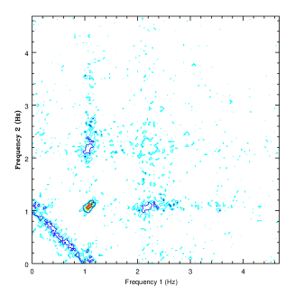
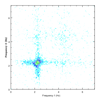
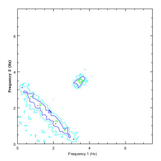
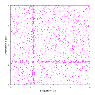
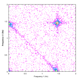
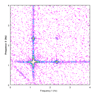
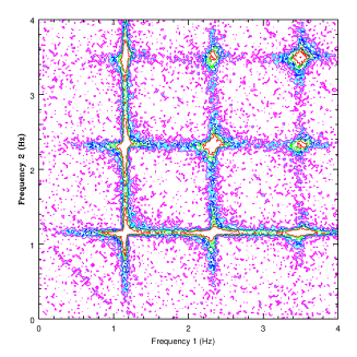
We have computed the bicoherence for many observations of GRS 1915+105. For the sake of brevity, we present only three representative results, aiming to present three observations with very similar power spectra, but qualitatively different bicoherences. We find three phenomenological patterns of variability here, which we described as “web”, “cross”, and “hypotenuse”. The bicoherences from actual data are plotted in figure 1, and the corresponding power spectra are plotted in figure 2.
4.1 The “cross” pattern
When the source is in the “radio quiet” state C at low count rates, the QPO frequency is low (less than 2 Hz). Here, the bicoherence shows a “cross” behavior (see the results from ObsID 20402-01-15-00 plotted in figure 1b for the bicoherence and figure 2b for the corresponding power spectrum), with large bicoherence for frequency pairs where one frequency is the QPO frequency and the other can take on any value. Here, in contrast to the web pattern, there is large bicoherence even for noise frequencies less than twice . Additional power is seen at the harmonics and for the harmonics interacting with the noise.
It is interesting to consider whether the cross pattern might be indicating the effects of very broad wings to the QPO, with no actual coupling between the QPO and the noise, but just coupling between the QPO and its harmonics. This is unlikely to be the case. Firstly, the bicoherence features are asymmetric in frequency space, while the QPOs are well-fit by Lorentzians, indicating that they are not asymmetric in frequency space. In principle, since the bicoherence is normalised by dividing by quantities related to the power spectrum, changes in the strength of the noise component, which would dilute the coupled variability, could be expected. In this case, though, there is both more power in the noise component of the power spectrum and stronger bicoherence at frequencies below the QPO frequency than above it. Secondly, the harmonics tend to follow either roughly circular patterns for their bicoherence, if the quasi-periodicity is caused by phase disconnections in an otherwise periodic signal, or patterns, if the quasi-periodicity is caused by the presence of many real frequencies due to changes in frequency over time or the superposition of multiple frequencies as might happen if the variability is due to orbital motions over a range of radii (see Maccarone & Schnittman 2005), and what is observed is different from both.
4.2 The “hypotenuse” pattern
At higher count rates of the “radio quiet” state C, the bicoherence pattern changes dramatically (see the results from ObsID 30184-01-01-000 plotted in figure 1c for the bicoherence and figure 2c for the corresponding power spectrum) . A high bicoherence is seen primarily where the two noise frequencies add up to the QPO frequency – that is, the regions of large bicoherence make a diagonal line. We refer to this as the “hypotenuse” pattern because the region of strong bicoherence forms the hypotenuse of a triangle with its other two sides being the axes of the plot. The “hypotenuse” pattern typically also shows a roughly circular spot of high bicoherence with ==, since there is power both at the fundamental and at the first harmonic and these two variability components are coupled. A few other observations at similar count rates and with similar QPO frequencies in the non-plateau state have been examined, and show the same qualitative features in their bicoherences. We also note that the diagonal elongation in the bicoherence plot from lower left to upper right for is likely to be related to the frequency drift during the observation that is mentioned above.
4.3 The “web” pattern
A hybrid class of bicoherence plots can be seen for some of the observations, where features resembling those seen in the “cross” and of the “hypotenuse” patterns can be seen together. When the source is in the radio plateau state, as in ObsID 10408-01-25-00, the bicoherence shows a rather strong signal for two combinations (see figure 1a and figure 2a for the corresponding power spectrum) – a diagonal line from upper left to lower right, with , for all . Additionally, one vertical/horizontal streak is seen with one of the frequencies equal to the QPO frequency, and the other a frequency greater than the twice QPO frequency. No significant vertical/horizontal signal is seen for the case that . The value of the bicoherence tapers off for frequencies where the power in the noise component becomes small. We refer to this pattern of behavior as the “web” pattern. A few other observations at similar count rates in the plateau state have been examined, and show the same qualitative features in their bicoherences.
4.4 A few brief remarks on other observations
In some observations not plotted in this paper, with the highest count rates seen from GRS 1915+105 in its class, the bicoherence seems to tend towards zero entirely. However, at the highest count rates, the QPO frequency can also change substantially on the timescale of a single RXTE observation. The bicoherence is not well suited to dealing with data sets which are non-stationary in this manner. This problem may exist even in some of the lower count rate data sets, but at a much lower level. We note that in a few of the observations, the bicoherence is extended along the line around the location where the interactions are between the QPO and its first harmonic – this effect can be seen showing up weakly in Figure 1a. It was shown in Maccarone & Schnittman (2005) that this is characteristic of a QPO which is broadened due to the existence of power at many frequencies, rather than due to phase disconnections.
5 Discussion
The overall values of the bicoherence in these data can also give us some clues as to the types of processes that might be producing the phase correlations. The bicoherence relates the instantaneous response of the driven oscillation to changes in the driving modes. As stated above, Greb & Rusbridge (1988) have shown that the maximum value of the squared bicoherence is /, where is the frequency resolution in the observation (or the width of a QPO, if the QPO is resolved), and is the frequency width of the driving spectrum. Therefore, if a QPO is driven by interactions of all noise frequencies less than the QPO frequency, then the largest possible value of the squared bicoherence is , where is the quality factor of the QPO.
Greb & Rusbridge (1988) also consider the effects of having a relatively narrow resonance. In this case, the squared bicoherence is reduced by a factor of the ratio of the coherence time in the driven mode to that in the driving mode. Thus, for resonant modes, which remain coherent for long periods of time relative to the timescale on which the driving signal remains coherent, the bicoherence will be substantially reduced. This can be grasped intuitively in a qualitative sense – a strong resonance will have an amplitude related to the integral of the power dumped into it over a long timescale, and hence not strongly correlated with the instantaneous driving power.
In our observations, the values of the QPOs are typically , and the QPOs are overresolved in frequency space by factors of about 10-20. This yields expected maxima for the squared bicoherence of 0.05 (with the exact value depending both on which observation is considered, and whether multiple noise components interact nonlinearly to produce the QPO, or the QPO interacts nonlinearly with one noise component to produce another noise component). Larger values are possible for the harmonics of the QPOs, where the width of the driving spectrum is smaller than the width of the noise component in frequency space.
If we assume that the perturbations which are coupled to one another give an X-ray count rate which is linearly proportional to the amplitude of the perturbation, we can then use the magnitude of the bicoherence to gain some insight into whether the interactions can be through a narrow resonance at the QPO frequency. Our findings that the maximum values of the squared bicoherence for the cases where the QPO and the noise are interacting are would then imply that the coupling between the noise and QPO is relatively close to its maximal value. This places some immediate constraints on the classes of models which can be considered – models must have a large fraction of the power coming from an emission region which behaves as a single “system”, and, if the interactions between noise components produce a QPO through a resonant interaction, it must be a highly damped resonance.
5.1 Simulated light curve analysis
We now consider several different mathematical forms for light curves which correspond, at least approximately, to physical scenarios for producing QPOs and noise components which are correlated in some manner. We show that these different models can produce relatively similar power spectra while producing bicoherence diagrams which are qualitatively quite different from one another. Two of the patterns of behaviour found – the “cross” and the “hypotenuse” – are reproduced reasonably well by relatively straightforward models. The third, the “web” is only approximately reproduced here with a relatively simple model.
5.1.1 Bicoherence in terms of reservoir models
Where the bicoherence’s value is large, the variability must be coupled on the three timescales corresponding to the three frequencies included for the computation of the bicoherence. A natural way to couple variability on different timescales is with a reservoir model, where there are multiple variability components that drain the same reservoir. In this way, the different components “compete” for power – when the noise component becomes stronger, there will be less energy in the reservoir available for the QPO and vice versa, leading to a phase coupling. An analogous idea has been put forth to explain the coupling between optical variability and X-ray variability in XTE J1118+480 (Malzac, Merloni & Fabian 2004).
To determine what the output light curve will look like for the simulations, we define, in each case, two power spectra to use as outputs. One, the noise component, is a broad Lorentzian with a peak frequency of zero. The other, the quasi-periodic oscillation, is a much narrower Lorentzian with a peak at a higher frequency (we use here, where is the quality factor of the Lorentzian). The time series for these components are made using the method of Timmer & König (1995). This method generates simulated times series from a power spectrum under the assumption that the process is Gaussian – thus we can be assured that any non-linearity we detect is because of the physics we put in after generating the initial random time series.
Then, a reservoir is defined. Energy is injected into the reservoir either at a constant rate, or at a purely random rate (i.e. a random number uniformly distributed between zero and one times a normalisation). Energy is drawn from the reservoir by each of the two components. The flux of a component is taken to be the value of its time series multiplied by the size of the reservoir at that instant times some normalization. The flux is then subtracted from the reservoir. Specifically, we do the following:
| (3) |
where is the size of the reservoir at time , after the energy injection has taken place, but before the draining of the reservoir has taken place, is the time step, is the size of the energy reservoir at the end of the previous time step, and is the injection rate into the reservoir per time step;
| (4) |
where is the output flux from the QPO component, is the time series of the QPO produced by the Timmer & König method, and is a normalization constant;
| (5) |
where is the output flux from the noise component, is the time series of the noise produced by the Timmer & König method, and is a normalization constant; and, finally,
| (6) |
Two general cases are considered, and we search a range of parameter space for each case. The first is where the output “light curve” is the sum of the fluxes of the two components. This might correspond to a case where accretion power is dissipated either in some oscillating region which produces the QPO, or a non-resonant part of the accretion disc, which produces the noise component. The second is where the output light curve is only the QPO’s flux. This might correspond to the case where the broad Lorentzian represents a jet which extracts power from the system, but does not emit in the X-rays (see e.g. Malzac et al. 2004).
If the reservoir is drained by a component which does not contribute to the X-ray light curve, then the size of the reservoir in “view” of the X-ray light curve, will effectively be some quantity minus the integral of the power drained by the other component. As a result, the reservoir itself will have a signature of its modulation, so when the output light curve is obtained by multiplying the reservoir size by the time series for the QPO, the “QPO” component will now be modulated on the timescale of the “noise,” and the noise power spectrum will affect final power spectrum. As we show below, the qualitative properties of the bicoherence are largely the same regardless of whether the two drains on the energy reservoir both contribute to the output flux, or only one of these does. Again, the logic we follow here is quite similar to that in Malzac et al. (2004). Given that, as we will show below, these models seem to match the data for the plateau states more closely than the more radio quiet states, it would not be surprising if energy extraction by a jet were an important factor in determining the properties of the light curve.
After the basic model equations are defined, a time series is produced for the model. The QPO and noise components are produced as time series using the Timmer & König method, with both components assumed to be Lorentzians with parameter values set to values similar to those seen in the data for various observations. For a very small number of time bins, the value of one of these time series will be negative, in which case we set it to zero. Alternatively, the energy extracted in a time interval may be larger than the size of the reservoir, in which case we set the power such that the whole reservoir is drained in that time step.
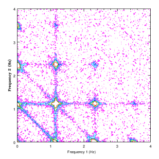
When the amplitude of variability is large, the reservoir’s level fluctuates strongly. This leads to the production of harmonics in the QPO (since the oscillations become non-sinusoidal when the reservoir fluctuates in response to the oscillations themselves). It also leads to phase coupling of all types between the QPO and the noise. This produces a “web-like” pattern in the bicoherence; however, the web-like pattern here is not identical to the one seen in the radio plateau state. In the real data, the “cross-like” structures begin to manifest themselves only for noise frequencies larger than the frequency of the first harmonic, while in these simulations, the cross structures appear at all noise frequencies. Furthermore, in some of the simulations, there are diagonals from upper left to lower right related to the cross structure which are strong features at all frequencies adding up to at least one of the harmonics. These are not present in the real data. The strong diagonals manifest themselves when the total variability in the reservoir is dominated by the noise component, rather than by the QPO. The model bicoherence is shown in Figure 3b to represent a case where the jet extracts power (i.e. so that the extracted noise-component power does not lead directly to observed emission), and in Figure 4b for the case where the noise component is added back in to the model light curve. Figure 5b shows the simulated power spectrum corresponding to the bicoherence shown in Figure 3b.
In the numerical calculations where the noise component is not added to the final light curve, the QPO has a mean count rate of 8000, with a root mean squared variability level of 1200, while the noise component has a mean value of 20000, with an root mean squared variability level of 8000. We re-fill the reservoir by adding a random number drawn from a uniform distribution between 0 and 8000. The draining of the reservoir takes place by summing the two time series, multiplying by the size of the reservoir, dividing 200000, and subtracting that from the reservoir value.
Where the noise component is added to the final light curve, a slightly different procedure is adopted. The QPO and noise components are added together in the initial power spectrum made before the inversion into a time series using the Timmer & König method. The QPO is given a normalization in the power spectrum 200 times higher than the noise component’s. The actual value in the final power spectrum comes from converting this power spectrum into a time series with mean value of 8000 and rms amplitude of 6000. All other procedures are as above.
At low variability amplitude, only the cross-like structures are seen strongly, although a weak “hypotenuse” feature is still present when the noise component is added to the output “light curve.” The bicoherence is shown without the noise component added back in in Figure 3a, and with it added back in in Figure 4a. The power spectrum corresponding to the low variability amplitude model is shown in Figure 5a. The simulated bicoherence plots in this case look quite a bit like the bicoherence plot seen from observation 20402-01-15-00 (compare the observational data in Figure 1b with the simulations in Figure 3a).
The procedure for converting the model into a simulated light curve is the same as above, except for some changes in values of parameters. For the case where the noise component is not seen in the output simulated light curve, the noise component in this case has an rms amplitude of 1000 instead of 8000, with all other parameter values the same. Where the noise component is added to the final simulated light curve, the rms amplitude of the simulated light curve is 2500 instead of 6000.
5.1.2 Bicoherence in terms of damped forced harmonic oscillators
We have also considered the case of a damped, forced harmonic oscillator. This is conceptually similar to the mechanism suggested by Psaltis & Norman (2000) for producing both quasi-periodic oscillations and noise components from a single perturbation spectrum – the quasi-periodic oscillation appears at the resonant frequency of the system, while a white noise input spectrum is turned into a red noise component by the fact that damped oscillators act as low-pass filters. However, the response of the system was considered to be linear in that work, meaning that non-linear features like non-zero bicoherence can not be explained without some modifications. When modifying the system of equations, to allow for a non-linear restoring force, we find that the resulting pattern of bicoherence that results from this scenario is relatively similar to the “hypotenuse” pattern, although we do have trouble reproducing a strong bicoherence with a realistic power spectrum. An alternative physical mechanism for producing such a quasi-periodic oscillation would be to have variations in the accretion rate excite inertial-acoustic modes in the inner accretion disc (Chen & Taam 1992;1995).
Quantitatively, this scenario is modelled in the same way as a spring which does not follow Hooke’s Law (i.e. ), but rather has an asymmetric, higher order restoring force, which is given by , where is the displacement, and and are constants parameterizing the strength of the restoring force. If , this does reduce to Hooke’s Law, and the lack of a non-linear term leads to a lack of observable features in the bicoherence plot.
The full equations of motion for this “oscillator” are:
| (7) |
where is the damping coefficient and is the magnitude of the driving force, which is assumed to be a white noise process;
| (8) |
where is the mass of the oscillator, which we set to unity for these calculations, and is 0.001. The calculated simulated light curve is the time series , and has 1048576 points. The bicoherence is computed from 256 chunks of 4096 points.
For the first calculation, we set the parameter values to and . We show the plot of simulated data in 3c. We note there is one substantial difference between the model data and the real data for 30184-01-01-000, which is that the model data has stronger bicoherence along the “hypotenuse” when the two frequencies are most different from one another, while the real data shows the opposite trend. This trend makes the model values more seriously deviant from the real data for the strongest damping of the motion of the oscillator.
When the damping factor is very low, then the resulting bicoherence plots can look quite similar to the “web” pattern. In figure 6, we show the power spectrum and bicoherence plot for a low damping case. The calculations are done in the same manner as the ones described in the previous paragraph, except with =0.25 and . For values of intermediate between 0.6 and 7.0, the “hypotenuse” can become much broader without creating such strong additional harmonics in the power spectrum. This simulation, like the one whose power spectrum and bicoherence are shown in Figures 45b and 3b, respectively, matches many of the properties of the data, but not all; however, here, the problem is primarily that the model shows too strong a bicoherence in streaks where there is only noise, rather than power in the QPO or its harmonics.




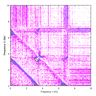
5.1.3 Caveats
There are further steps which will be needed to make models which match all the statistical properties of the observed light curves. For example, in most cases, the observed flux distributions will follow a log-normal distribution (Uttley et al. 2005) - we do not attempt here to enforce this requirement. We do note that it was found by Uttley et al. (2005) that exponentiating the flux values in a light curve can push a flux distribution towards a log-normal distribution. We have done this in a few cases, and have found that the bicoherence plots change very little when the flux values are exponentiated. Uttley et al. (2005) have already shown that power spectra are not typically affected strongly by this transformation. Therefore, flux distributions and bicoherence plots are largely independent tests of the variability’s coupling, although the flux distributions produced in these simulated data sets do not deviate strongly from log-normal distributions in any event. Furthermore, in cases where there are strong QPOs with very low frequencies, there are clear deviations of the flux distribution from being log-normal (Misra et al. 2006). We have additionally not ensured that the power spectra of real observations are matched exactly by these simulations. In essence, since the input models do not have any radiative transfer in them, we are assuming that the radiative efficiency of any perturbation will be constant when we call the output time series “simulated light curves.” Deviations from this assumption are likely to affect the power spectra, and, especially, the flux distributions, far more seriously than they affect the morphology of the bicoherence plots. Such deviations are quite easy to imagine in situations where there exists a resonance.
An additional potential problem exists with connecting the toy models presented here to reality. Much of the phenomenology appears to be similar between the different sub-types of classes. It would therefore be surprising if there were a qualitative change in the mechanism for producing the QPOs. It would thus be useful to identify a means to unite the different mechanisms described here, or to develop an entirely new physical model to explain all the observed phenomenology in a more unified way, with just the change of one or two parameters causing the broad range of phenomena seen in terms of bicoherence patterns.
6 Conclusions
We have shown clearly that the variability in the noise components and quasi-periodic oscillations of GRS 1915+105 are correlated with one another. The bicoherence provides a good discriminator among variability models which produce similar power spectra through quite different physical processes. We have found that it is plausible that in the “plateau” state of GRS 1915+105, the variability is caused by a reservoir of energy being drained by a noise component (which could be the radio jet) and a quasi-periodic component, while in the brighter part of the state, the variability is consistent with a white noise input spectrum driving a damped harmonic oscillator with a non-linear restoring force. While the models presented here are almost certainly not unique solutions for what is occuring physically in these systems, it is quite clear that the bicoherence will provide excellent constraints on more physically motivated models for the variability, and that we can definitely identify cases where the properties of the power spectra are quite similar, but the properties of the light curves are quite different.
7 Acknowledgments
We are grateful to Ron Elsner for sending us an unpublished draft written by himself, R. Bussard and M. Weisskopf many years ago discussing some of the fundamental properties of the bispectrum, and to Patricia Arévalo, Mike Nowak and Simon Vaughan for useful discussions related to variability statistics, and to Marc Klein-Wolt, Mariano Méndez and Luciano Rezzolla for more general, but equally interesting discussions, and to Rob Fender for helping to clarify some of the nomenclature surrounding GRS 1915+105, and Tomaso Belloni for useful comments on a draft of the paper. We also thank the anonymous referee for some useful suggestions which have hopefully improved the clarity of the paper. TJM also wishes to thank Dave Smith of the Quantum and Functional Matter group in the Southampton School of Physics and Astronomy for useful discussions.
References
- [1] Abramowicz M.A., Kluzniak W., 2001, A&A, 374L, 19
- [2] Belloni T., Klein-Wolt M., Méndez M., van der Klis M., van Paradijs J., 2000, A&A, 355, 271
- [3] Belloni T., Psaltis D., van der Klis M., 2002, ApJ, 572, 392
- [4] Chen, X. & Taam, R.E., 1992, MNRAS, 255, 51
- [5] Chen, X. & Taam, R.E., 1995, ApJ, 441, 354
- [6] Fackrell, J 1996, Ph.D. Thesis, University of Edinburgh
- [7] Fender R. & Belloni T., 2004, ARA&A, 42, 317
- [8] Foster, R.S., Waltman, E.B., Tavani, M., Harmon, B.A., Zhang, S.N., Peciesas, W.S. & Ghigo, F.D., 1996, ApJL, 467, 81
- [9] Giannios D., Spruit H.C., 2004, A&A, 251
- [10] Greb, U. & Rusbridge, M.G., 1988a, Plasma Physics and Controlled Fusion, 30, 537
- [11] Hinich M., Wolinsky M., 2005, Journal of Statistical Planning and Inference, 130, 405
- [12] Homan J., Belloni T., 2005, Ap&SS, 300, 107
- [13] Kim Y.C., Powers E.J., 1979, IEEE Transactions on Plasma Science, Vol. PS-7, Issue 2, 120
- [14] Kylafis N.D., Klimis G.S., 1987, ApJ, 323, 678
- [15] Lochner, J.C., Swank, J.H., Szymkowiak, A.E., 1989, ApJ, 337, 823
- [16] Lyubarskii Y.E., 1997, MNRAS, 296, 696
- [17] Maccarone, T.J. & Coppi, P.S., 2002, 336, 817
- [18] Maccarone T.J., Schnittman J.D., 2005, MNRAS, 357, 12
- [19] Malzac, J., Merloni, A., & Fabian, A.C., 2004, MNRAS, 351, 253
- [20] Mauche, C.W., 2002, ApJ, 580, 423
- [21] Mendel, J. 1991, Proc IEEE, 79, 278
- [22] Merloni, A. & Fabian, A.C., 2001, MNRAS, 321, 549
- [23] Misra R., Harikrishnan K.P., Mukhopadhyay B., Ambika G., Kembhavi A.K., 2004, ApJ, 609, 313
- [24] Misra R., Harikrishnan K.P., Ambika G., Kembhavi K., 2006, ApJ, 643, 1114
- [25] Muno, M.P., Remillard, R.A., Morgan, E.H., Waltman, E.B., Dhawan, V., Hjellming, R.M. & Pooley, G., 2001, ApJ, 556, 515
- [26] Nowak, M.A. & Vaughan, B.A., 1996, MNRAS, 280, 227
- [27] Nowak, M.A., 2000, MNRAS, 318, 361
- [28] Olive J.F., Barret D., Boirin L., Grindlay J.E., Swank J.H., Smale A.P., 1998, A&A, 333, 942
- [29] Pottschmidt,K., Wilms, J., Nowak, M.A., Pooley, G.G., Gleissner, T., Heindl, W.A., Smith, D.M., Remillard, R. & Staubert, R., 2003, A&A, 407, 1039
- [30] Priedhorsky,W., Garmire, G.P., Rothschild, R., Boldt,E., Serlemitsos, P., Holt, S., 1979, ApJ, 233, 350
- [31] Psaltis, D., Belloni, T. & van der Klis, M., 1999, ApJ, 520, 262
- [32] Psaltis D., Norman C., 2000, astro-ph/0001391
- [33] Rezzolla L., Yoshisa S’i., Maccarone T.J., Zanotti O., 2003, MNRAS, 344L, 37
- [34] Schnittman J.D., Bertschinger E., 2004, ApJ, 606, 1098
- [35] Takeuchi, M., Mineshige, S., Negoro, H., 1995, PASJ, 47, 617
- [36] Takeuchi, M., Mineshige, S., 1997, ApJ, 486, 160
- [37] Terrell, N.J., 1972, ApJL, 174L, 35
- [38] Timmer J., König M., 1995, A&A, 300, 707
- [39] Timmer, J., Schwarz, U., Voss, H.U., Wardinski, I., Belloni, T., Hasinger, G., van der Klis, M. & Kurths, J., 2000, PhRvE, 61, 1342
- [40] Uttley, P. & McHardy, I.M., 2001, MNRAS, 323L, 26
- [41] Uttley P., McHardy I.M., Vaughan S., 2005, 359, 345
- [42] van Straaten, S., van der Klis, M., Di Salvo, T., Belloni, T., 2002, ApJ, 568, 912
- [43] Warner B., Woudt P.A., Pretorius M.L., 2003, MNRAS, 344, 1193
- [44] Wijnands, R. & van der Klis, M., 1999, ApJ, 514, 939