Second order closure for stratified convection: bulk region and overshooting

Abstract

The parameterization of small-scale turbulent fluctuations in convective systems and in the presence of strong stratification is a key issue for many applied problems in oceanography, atmospheric science and planetology. In the presence of stratification, one needs to cope with bulk turbulent fluctuations and with inversion regions, where temperature, density –or both– develop highly nonlinear mean profiles due to the interactions between the turbulent boundary layer and the unmixed –stable– flow above/below it. We present a second order closure able to cope simultaneously with both bulk and boundary layer regions, and we test it against high-resolution state-of-the-art 2D numerical simulations in a convective and stratified belt for values of the Rayleigh number, up to $Ra\sim 10^{9}$. Data are taken from a Rayleigh-Taylor system confined by the existence of an adiabatic gradient.

Realistic parameterization of convective regions in presence of strong stratification is a problem of interest for the evolution of the convective boundary layer in fields as different as atmospheric science Siebesma07 , stellar convection rt_atmosphere ; Ludwig99 and oceanography Large94 ; Burchard01 ; Canuto ; Wirth . The problem is intriguing also from a pure theoretical point of view: one would like to predict the interplay between buoyancy and turbulence at the edge between a convective region and a stable stratified volume above/below it. Due to turbulent activity, intermittent puffs of temperature, density and momentum tend to enter the stably stratified region, locally producing an inversion in the energy balance: kinetic energy is indeed lost, as potential energy is increased. Those turbulent puffs are the result of intense plumes traveling across the volume, often generated in the bottom layer, producing a “non-local” interaction between edge and bulk of the turbulent medium. The problem, already recognized in the early 50’s Vitense53 ; spiegel3 , is still a subject of intense research (see e.g. Burchard01 ). Recent studies have shown that, in the absence of strong stratification, mixing length theory based on Prandtl or Spiegel closure works very well in situations as different as for the case of Rayleigh-Taylor systems boffetta.prl.2010 or in fluid mixing by gravity currents Ecke09 .

Figure 1: Right panel: initial vertical density and temperature profiles. Left and middle panels: Vorticity and temperature snapshots with weak and strong stratification, respectively. Notice the free rising plumes in the left panel typical of non-stratified RT system. In the middle panel stratification is stronger and turbulence is confined below and above the unmixed fluid at rest: at the boundary the temperature profile overshoots.

Nevertheless, whenever strong stratification stops the evolution of the mixing profile, an overshooting region with temperature inversion develops and local closures fail. The problem arises from non-local effects caused by turbulent plumes or convective updraft.

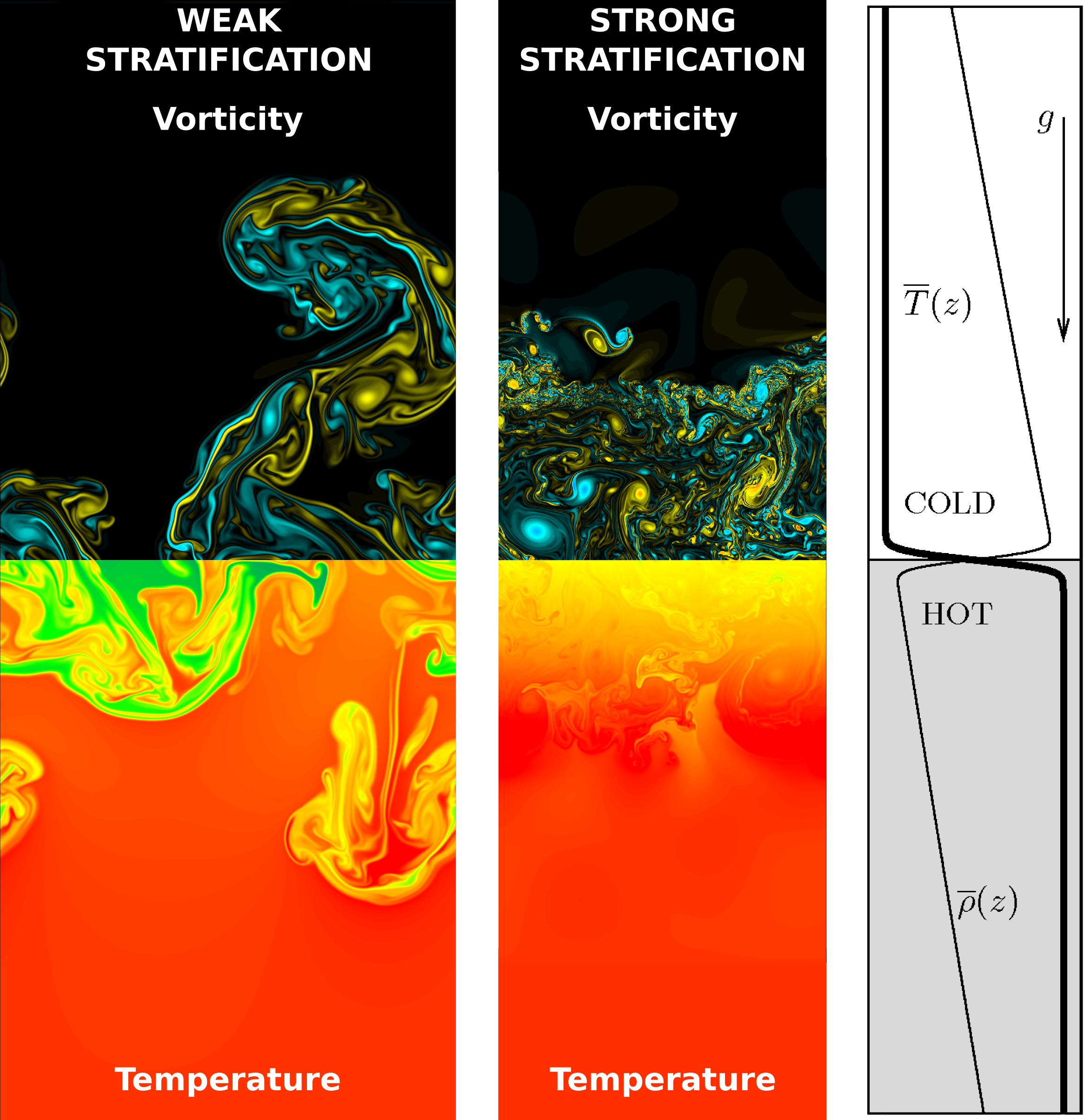
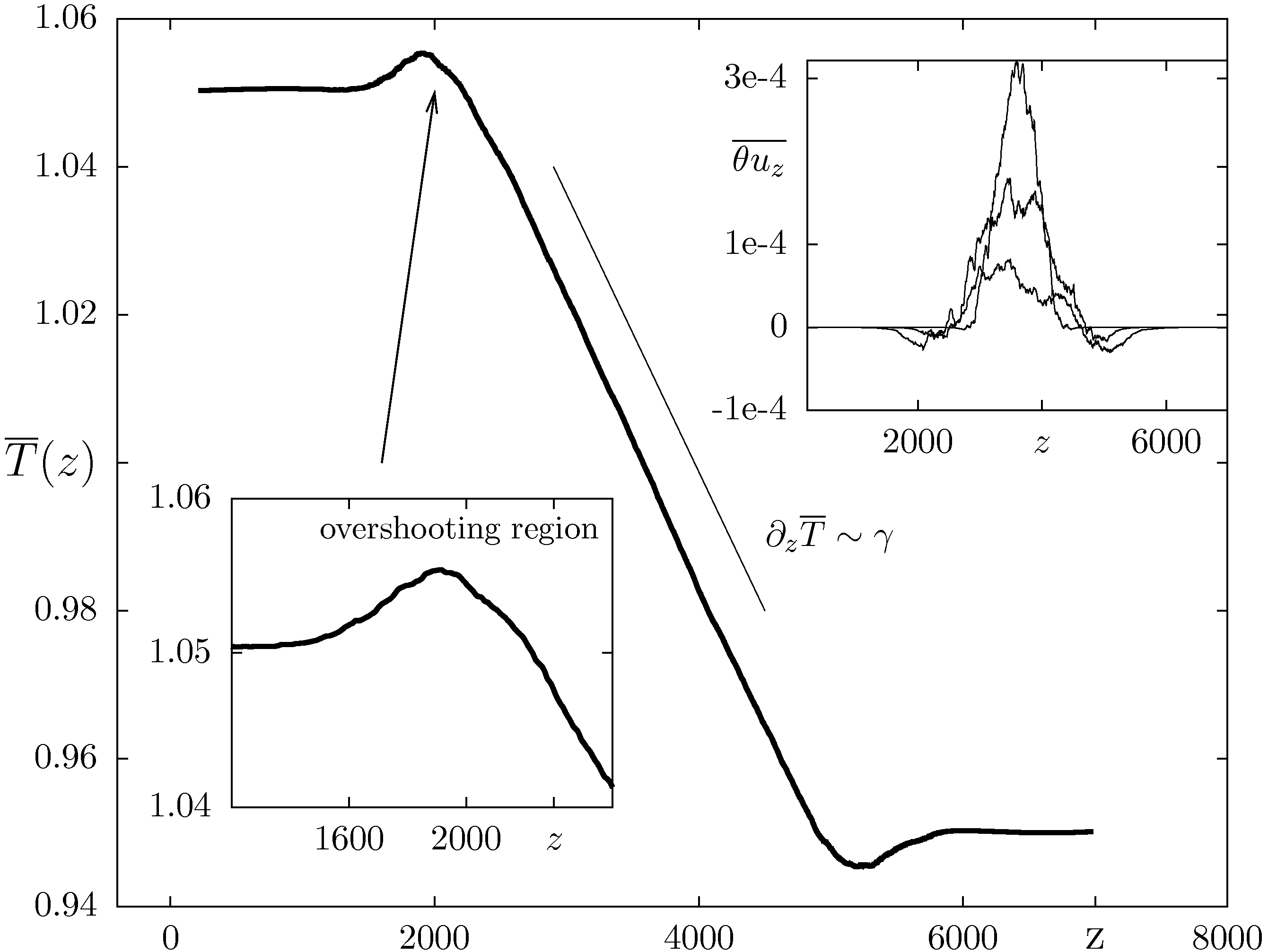
The situation can be visualized in the middle panel of Fig. 1 where a highly turbulent configuration is confined by two stably stratified media below and above it, at an effective Rayleigh number, $Ra\sim 10^{9}$. The mean temperature profile is linear in the bulk and it develops two –symmetric– overshooting regions at the edge between the turbulent boundary layer and the fluid at rest with the heat flux inverting sign (see Fig. 2). The configuration is obtained by evolving a Rayleigh-Taylor (RT) system in 2D with stratification chertkov ; celani1 ; pof1 ; detlef_arfm ; rt.temp ; cabot . The evolution of the RT mixing layer, unbounded in the absence of stratification, is stopped because of the adiabatic gradient, i.e. when the mean profile of the potential temperature becomes flat. In this letter we propose a closure for the evolution of the mixing layer, able to capture both the initial transient (free of any stratification effect) and the late slowing down and stopping due to stratification effects. The main idea is to go beyond single point closure for the mean temperature evolution, keeping itexact and closing only for second order quantities: the Reynolds stresses, the heat flux and temperature fluctuations, see e.g. Burchard01 .

Figure 2: RUN (B). Mean temperature profile $\overline{T}(z)$ after the RT evolution has stopped at the adiabatic slope (solid line). Bottom left panel: zoom of the overshooting region, with temperature inversion. Top right inset: heat flux profile $\overline{u_{z}\theta}(z)$ at three times before, during and after stopping: two regions develp with negative heat flux in correspondence of the temperature overshooting.

We test our closure against state-of-the-art numerical simulations at high resolution. We choose to work in a 2D geometry to maximize the capability to get quantitative measurements at high Reynolds and Rayleigh numbers. Choosing a RT system presents the extra complexity of non-stationarity, allowing to probe also turbulent time scales. Our numerical simulations are performed using a recently proposed thermal Lattice Boltzmann Method JFM.nostro able to reproduce the Navier-Stokes equations for momentum, density and internal energy. Validation of the method can be found in pof1 . Here we present numerical simulations up to $4096\times 10000$ grid points. Table I provides details of our numerical experiment, obtained running on the QPACE supercomputer qpace1 . We limit our discussion here to the case of an ideal gas, with the equation of state $P=\rho T$, and at small Mach number. In this case, the main effect of stratification is limited to the presence of an adiabatic gradient affecting the evolution of temperature spiegel3 . The equations are the following: (double indexes are summed):

$$\begin{cases}\partial_{t}u_{i}+u_{j}\partial_{j}u_{i}=-\frac{\partial_{i}p}{\rho_{m}}-\delta_{i,z}g\frac{\theta}{T_{m}}+\nu\partial_{jj}u_{i};\qquad i=x,z\\ \partial_{t}T+u_{j}\partial_{j}T-u_{z}\gamma=\kappa\partial_{jj}T;\\ \end{cases}$$ (1)

where $p$ is the deviation of pressure from the hydrostatic profile, $p=P-P_{H}$ and $\partial_{z}P_{H}=-g\rho_{H}$, $T_{m}$ and $\rho_{m}$ are the mean temperature and density in the system, $g$ is gravity and the adiabatic gradient is given by its ideal gas expression $\gamma=-g/c_{p}$ with $c_{p}$ the specific heat.

	$L_{x}$	$L_{z}$	$\gamma$	$Ra_{max}$	$N_{conf}$	$L_{\gamma}$	$t_{RT}$
(A)	$4096$	$10000$	$-1\cdot 10^{-5}$	$8\cdot 10^{9}$	$18$	$10000$	$6.4\cdot 10^{4}$
(B)	$3072$	$7200$	$-4.2\cdot 10^{-5}$	$3\cdot 10^{9}$	$11$	$2408$	$2.7\cdot 10^{4}$

Table 1: Run (A): weak stratification. Run (B) strong stratification. Adiabatic gradient: $\gamma=-g/c_{p}$; $c_{p}=2$. Adiabatic length in grid units: $L_{\gamma}=\Delta T/|\gamma|$, $\Delta T=T_{down}-T_{up}$, $T_{m}=(T_{down}+T_{up})/2$ and $T_{up}=0.95$, $T_{down}=1.05$. Rayleigh number in presence of stratification is defined as spiegel3 : $Ra(t)=gL(t)^{4}(\Delta T/L(t)+\gamma)/(\nu\,\kappa)$). Maximal value is obtained when $L(t)=3/4L_{\gamma}$. Number of independent runs with random initial perturbation: $N_{conf}$. Atwood number = $At=\Delta T/(2\,T_{m})=0.05$. Characteristic time scale, $t_{RT}=\sqrt{L_{x}/(gAt)}$.

In this Boussinesq approximation spiegel3 for stratified flows, momentum is forced only by temperature fluctuations $\theta=T-\bar{T}$ where we use the symbol $\overline{(\cdot)}$ to indicate an average over the horizontal statistically-homogeneous direction.

Figure 3: Evolution of the mixing layer extension $L(t)$ for both run (A) and (B). Notice the stop by stratification effects for the latter. Solid lines correspond to the closure prediction for the mixing length evolution obtained with the choice $[1.45,4.5]$ (run A) and $[0.3,6.5]$ (run B) for the parameters $[b_{\theta},b_{\theta u_{z}}]$ (see text). We also show 5 consecutive snapshots of the overshooting region highlighting the formation of a turbulent plume trying to enter the stable region and rejected back by gravitational forces.

The initial configuration is given by two regions of cold (top) and hot (bottom) fluids prepared in the two half volumes of our cell (see right panel of Fig.1); turbulence is triggered by a small perturbation of the interface between them rt.review (see boffi for a recent high resolution study of the classical RT system in 3D).
From (1), one easily derives the equations for the mean temperature profile, total kinetic energy, heat flux and temperature fluctuations:

$$\begin{cases}\partial_{t}\overline{T}+\partial_{z}\overline{u_{z}\theta}=\kappa\partial_{zz}\overline{T}\\ \frac{1}{2}\partial_{t}\overline{\theta^{2}}+\frac{1}{2}\partial_{z}\overline{\theta^{2}u_{z}}+\overline{u_{z}\theta}(\partial_{z}\bar{T}-\gamma)=\kappa\overline{\theta\partial_{jj}\theta}\\ \frac{1}{2}\partial_{t}\overline{u^{2}}+\partial_{z}[\overline{u^{2}u_{z}}+\overline{u_{z}p}]=-g\overline{\theta u_{z}}-\epsilon_{\nu}\\ \partial_{t}\overline{\theta u_{z}}+\partial_{z}[\overline{\theta u_{z}^{2}}+\overline{\theta p}]=-g\overline{\theta^{2}}+\beta(z)\overline{u_{z}^{2}}-\epsilon_{\theta,u_{z}}\end{cases}$$ (2)

where $u^{2}=u_{x}^{2}+u_{z}^{2}$, $\beta(z)=(\partial_{z}\overline{T}-\gamma)$, and the dissipative terms are: $\epsilon_{\theta,u_{z}}=(\nu+\kappa)\overline{\partial_{i}\theta\partial_{i}u_{z}}$, $\epsilon_{\theta}=\kappa\overline{\partial_{i}\theta\partial_{i}\theta}$, $\epsilon_{\nu}=\nu\overline{\partial_{i}u_{j}\partial_{i}u_{j}}$. The above set of equations is exact, except for boundary dissipative contributions as for example, $\kappa\partial_{z}\overline{\theta\partial_{z}\theta}$ which are irrelevant when $\kappa,\nu\rightarrow 0$ in absence of walls. From the second of (2) it is evident that temperature fluctuations are not forced anymore as soon as the mixing region develops a mean temperature profile of the order of the adiabatic gradient:

$$\partial_{z}\overline{T}\sim\gamma.$$ (3)

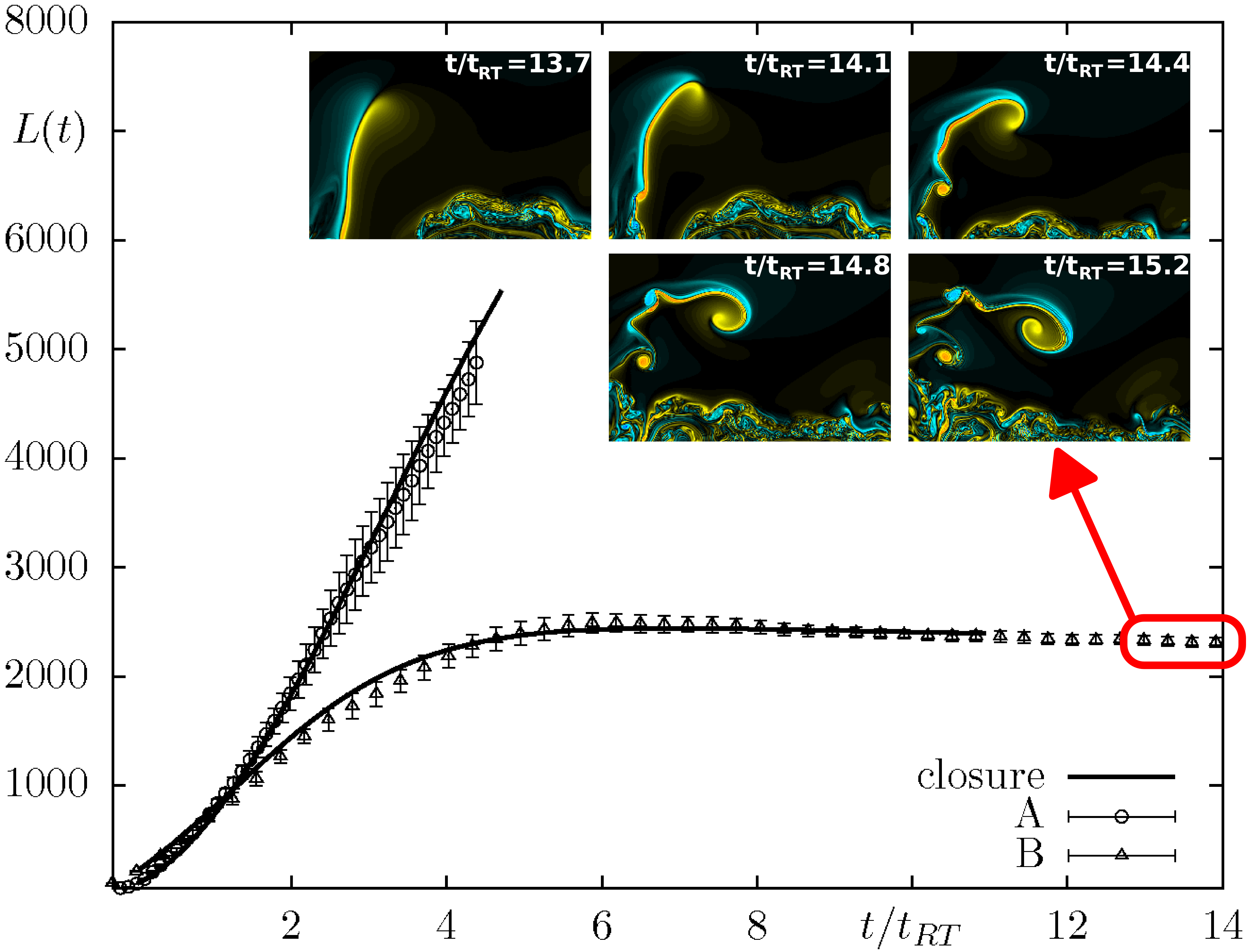
As a consequence, from that time on, turbulence will decline. Given $\gamma$, we can identify the adiabatic length, $L_{\gamma}=\Delta T/|\gamma|$ which corresponds to the prediction for the largest possible extension of the mixing layer during the RT evolution. In Fig. 3 we show the evolution of the mixing layer extension for two cases with weak (RUN A) and strong (RUN B) adiabatic gradient. Clearly, the extension of the mixing region stops to grow when $L(t)\sim L_{\gamma}$. In this paper we measure the mixing layer width $L(t)$ as in cabot :

$$L(t)=2\int dz\,\Theta\left[\frac{\overline{T}(z,t)-T_{up}}{T_{down}-T_{up}}\right],$$ (4)

with $\Theta[\xi]=2\xi;\;0\leq\xi\leq 1/2$ and $\Theta[\xi]=2\,(1-\xi);\;1/2\leq\xi\leq 1$. The overshoot developing at the edge between turbulent and unmixed fluid is visible in Fig. 2, where we show both the nonlinear temperature inversion (inset bottom left) and the corresponding inversion in the heat flux (inset top right). This overshooting region is clearly a problem for any attempt to close the mean profile evolution with any sort of local eddy diffusivity:

Figure 4: Check of the closure for the case with weak stratification (run A). Circles: numerical data, solid lines: clousre. We plot the local heat flux vs the local temperature mean gradient, $\overline{\theta u_{z}}$ vs $(\partial_{z}\overline{T})\times 10^{5}$, i.e. the effective diffusivity $K(z,t)$ (). Error bars are evaluated averaging over the configurations specified in table (1). Result from the closure is given by the solid line with $[b_{\theta},b_{\theta u_{z}}]=[1.45,4.5]$ and $b_{u_{z}}=0.03$. Inset: superposition of temperature profiles at three different times, $t/t_{RT}=2,4,5.5$ with the corresponding curves from the closure.

$$\overline{u_{z}\theta}=-K(z,t)\partial_{z}\overline{T}.$$

Different models have been proposed in the literature for $K(z,t)$, going from simple homogeneous closure ($K(z,t)\propto L(t)|\dot{L}(t)|$) to Prandtl-like mixing-length closure boffetta.prl.2010 ; Ecke09 ($K(z,t)\propto L(t)^{5/2}\partial_{z}\overline{T}$) or following Spiegel’s nonlinear approach spiegel3 ($K(z,t)\propto L(t)^{2}|\partial_{z}\bar{T}|^{1/2}$). All these attempts work well in the absence of overshooting and all of them suffer whenever an inversion in temperature and heat flux is observed (as in Fig. 2), implying a negative effective eddy diffusivity. In order to overcome this difficulty, we keep exact the equations for the mean profile and close only the fluctuations at the second order moments in (2).

Figure 5: Check of the closure for the case with strong stratification (run B). Circles: numerical data,solid line: closure.We plot the local heat flux vs the local temperature mean gradient, $\overline{\theta u_{z}}$ vs $(\partial_{z}\overline{T})\times 10^{5}$, i.e. the effective diffusivity $K(z,t)$ for two different times, $t=3\,t_{RT}$ (bottom panel); $t=6\,t_{RT}$ (top panel). Closure predictions ($[b_{\theta},b_{\theta u_{z}}]=[0.35;6.5]$) are given by the solid lines. Inset bottom panel: matching between the temperature profile and the closure. Inset top panel: overshooting region around the top boundary layer. The two lines correspond to the closure using two different choices, $[b_{\theta},b_{\theta u_{z}}]=[0.25;4.5];[0.35,6.5]$.

Considering $u_{z}\sim u$, we are left with six unknown to be defined: the three dissipative contributions on the rhs, and the three non-linear third order fluxes on the lhs. We close them adopting the simplest dimensionally-consistent local closure, for both fluxes and dissipative terms:

$$\begin{cases}\overline{\theta^{2}u_{z}}=a_{\theta}L|\dot{L}|\partial_{zz}\overline{\theta^{2}};\qquad\qquad\qquad\epsilon_{\theta}=b_{\theta}{\overline{\theta^{2}}}/{\tau(z,t)}\\ \overline{(u^{2}+p)u_{z}}=a_{u_{z}}L|\dot{L}|\partial_{zz}\overline{u_{z}^{2}};\qquad\epsilon_{\nu}=b_{u_{z}}{\overline{u_{z}^{2}}}/{\tau(z,t)}\\ \overline{\theta(u_{z}^{2}+p)}=a_{\theta u_{z}}L|\dot{L}|\partial_{zz}\overline{\theta u_{z}};\qquad\epsilon_{\theta,u_{z}}=b_{\theta u_{z}}{\overline{\theta u_{z}}}/{\tau(z,t)}\\ \end{cases}$$

where the typical time defining the dissipation rates is fixed by $\tau(z,t)=\sqrt{\overline{u_{z}^{2}}}/L(t)$. Some comments are in order. First, we notice that the closure is now local but on the second order moments, i.e. non-local for the evolution of mean profiles. Furthermore, out of the 6 free parameters, 4 can be handled quite robustly, all the three coefficients in front of the closure for third order quantities are set ${\cal O}(1)$ using a first order guess from the numerics, $a_{\theta}=0.2;a_{u_{z}}=0.3;a_{\theta u_{z}}=0.8$. Moreover, the free parameter defining the intensity of the kinetic dissipation, $\epsilon_{\nu}$, is irrelevant in 2D (absence of direct energy cascade). The only two delicate free parameters are those defining the intensities of temperature and heat-flux dissipative terms, $[b_{\theta},b_{\theta u_{z}}]$. In order to get a good agreement with the numerics we need some fine tuning for them. It is important to notice that both dissipative terms will develop a non-trivial vertical profile, i.e. they are not given by a simple bulk homogeneous parameterization.

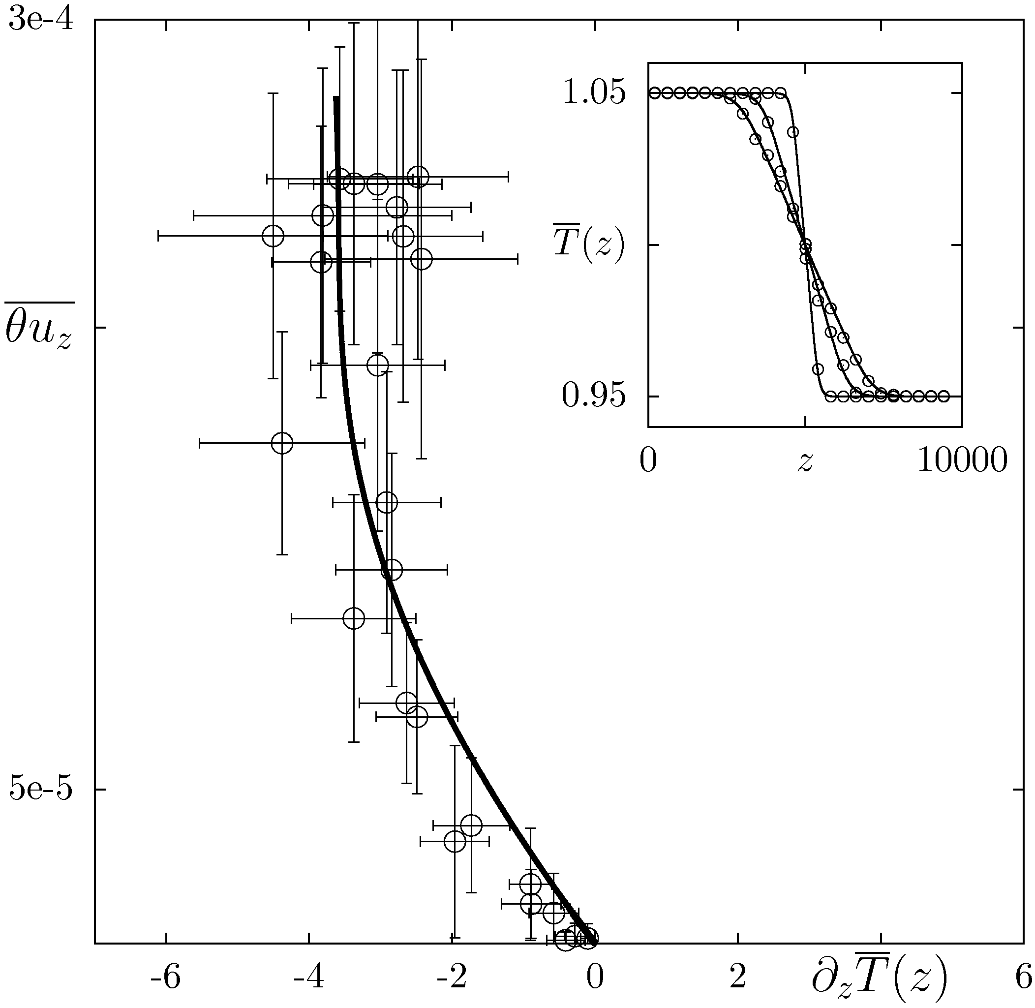
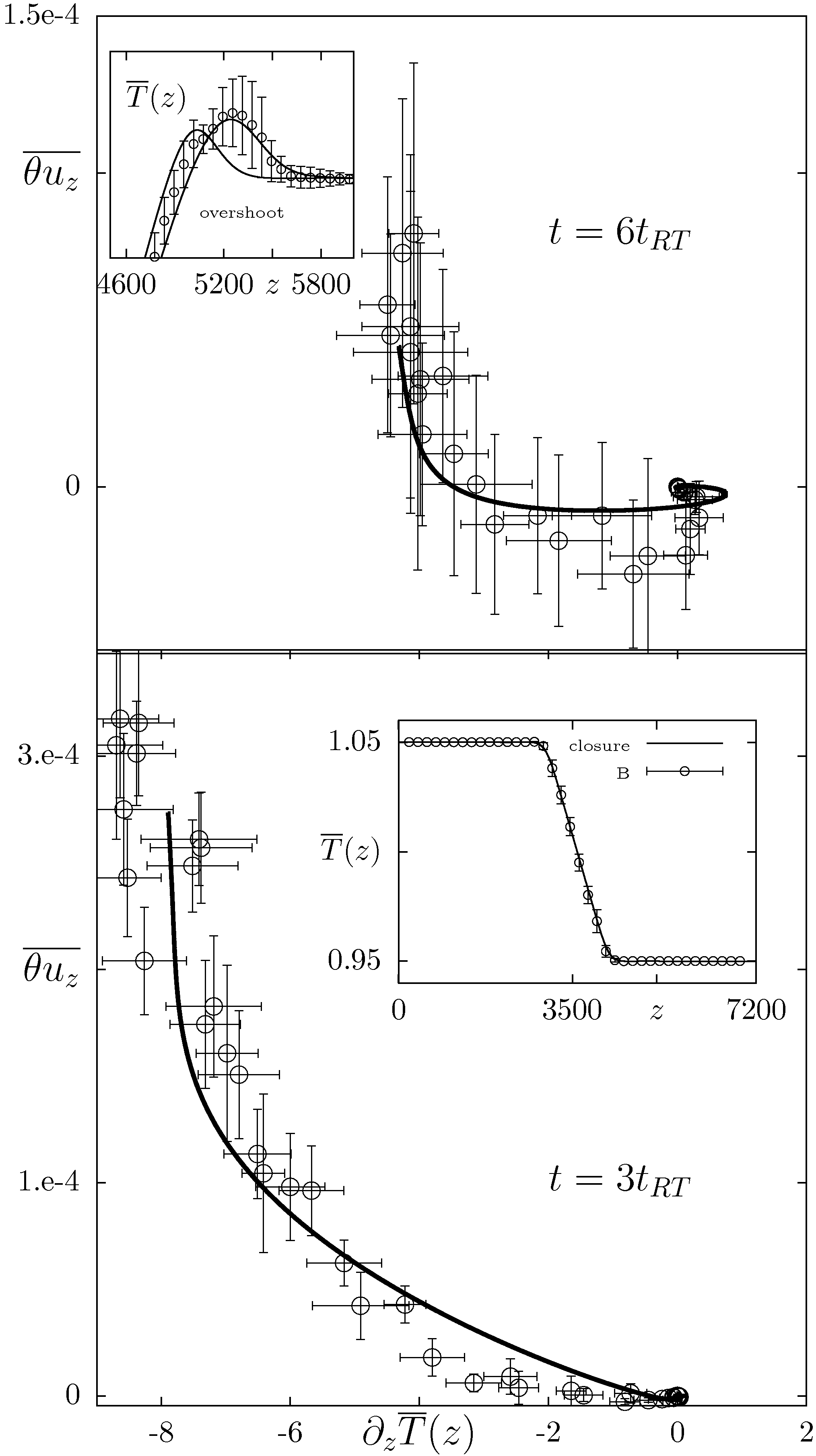
In Fig. 3 we show that the closure is able to reproduce quantitatively the evolution of $L(t)$ for both cases of weakly stratified turbulence (A) and strongly stratified case (B). In Figs. (4-5) we show the capability of the model to reproduce the heat flux vs. temperature profile behavior, providing a sort of aposteriori effective eddy diffusivity. As one can see, the closure is able to capture both the weak stratification case (Fig. 4) and the strong stratification case (Fig. 5). For the weak stratification case the aposteriori eddy diffusivity is very close to the one predicted by using the Prandtl mixing length theory as proposed in boffetta.prl.2010 or to the one proposed by Spiegel’s spiegel3 (not shown). For the strong stratification case, our model is able to capture also the long time behavior, even after the evolution has come to a halt due to the adiabatic gradient, where the heat flux has completely inverted sign, see top panel of Fig. 5. In the inset of the same figure we also show the capability of the closure to reproduce the overshooting profile. As one can see the agreement is very good and the results are not very sensitive to the choice of the free parameters.
We also remark that from eqs. (2) one may derive a dimensional closure neglecting all terms except the one at large scales, and assuming that temperature fluctuations are dominated by the global temperature jump: $\overline{\theta^{2}}\sim\Delta T$. From the third equation we derive: $\overline{\theta u_{z}}\sim L\overline{u_{z}^{2}}^{1/2}\partial_{z}\bar{T}$ and from the second: $\overline{u_{z}^{2}}\sim gL^{2}\partial_{z}\bar{T}$ that –combined together– leads to Spiegel’s closure: $\overline{\theta u_{z}}\sim L^{2}(\partial_{z}\bar{T})^{1/2}\partial_{z}\bar{T}$.

In conclusions, we have performed state-of-the-art 2D numerical simulations using a novel LBM for turbulent convection driven by a Rayleigh-Taylor instability in weakly and strongly stratified atmospheres. For the strongly stratified case, we are able to resolve the overshooting region with up to 800 grid points, something impossible to achieve with 3D direct numerical simulations because of lack of computing power. We have presented a second-order closure to describe the evolution of mean fields able to capture both bulk properties and the overshooting observed at the boundary between the stable and unstable regions. The closure is local in terms of fluctuations while keeping the evolution of the mean temperature profile exact. In order to apply the same closure to 3D cases one needs to take into account some possible non-trivial effects induced by the kinetic energy dissipation modeling, due to the presence of a forward energy cascade. As a result, also the parameter $b_{u_{z}}$ will become a relevant input in the model.

We acknowledge useful discussions with G. Boffetta and A. Wirth. We acknowledge access to QPACE and eQPACE during the bring-up phase of these systems. Parts of the simulations were also performed on CASPUR under HPC Grant 2009 and 2010.

References

- (1) A. Siebesma, P. M. M.Soares & J. Teixeira. J. Atmosph. Science 64 1230 (2007); A. Siebesma, J.W.M. Cuijpers. Journ. Atmosph. Science 52 650 (1995).
- (2) V.M. Canuto & J.Christensen-Dalsgaard, Annu. Rev. Fluid Mech 30, 167 (1998)
- (3) H.G. Ludwig, F. Allard and P.H. Hauschildt Astron. Astrophysics 459, 599 (2006); R. Trampedach Astrophys. Space Sci. 328 213 (2010).
- (4) W.G. Large, J.C. McWilliams & S.C. Doney, Review Geophys. 32, 363 (1994)
- (5) H. Burchard and K. Bolding, Journ. Phys. Ocean. 31 1943 (2001).
- (6) V.M. Canuto et al.Journ. Phys. Ocean. 32 240 (2002).
- (7) A. Wirth & B. Barnier Journ. Phys. Ocean. 38 803 (2008).
- (8) E. Vitense, Zs. f. Ap. 32, 135 (1953)
- (9) E.A. Spiegel Astrophys. J. 141, 1068 (1965); E.A. Spiegel & G. Veronis, Astrophys. J. 131, 442 (1960); E.A. Spiegel. Astrophys. J. 206, 536 (1976)
- (10) G. Boffetta, F. De Lillo & S. Musacchio, Phys. Rev. Lett. 104, 034505 (2010)
- (11) P. Odier et al. Phys. Rev. Lett 102 134504 (2009)
- (12) M. Chertkov, Phys. Rev. Lett. 91, 115001 (2003)
- (13) A. Celani, A. Mazzino & L. Vozella, Phys. Rev. Lett. 96, 134504 (2006)
- (14) A. Scagliarini et al. Phys. Fluids 22, 055101 (2010); L. Biferale et al. Phys. Fluids 22, 115112 (2010).
- (15) D. Lohse & K.Q. Xia, Annu. Rev. Fluid Mech. 42, 335 (2010)
- (16) T.T. Clark, Phys. Fluids 15, 2413 (2003); J.R. Ristorcelli & T.T. Clark, J. Fluid Mech. 507, 213 (2004)
- (17) W.H. Cabot and A.W. Cook Nature Phys. 2, 562 (2006)
- (18) M. Sbragaglia et al. J. Fluid Mech. 628, 299 (2009)
- (19) G. Goldrian et al. Computing in Science & Engineering, 10 46 (2008).
- (20) D.H. Sharp, Physica D 12, 3 (1984)
- (21) G. Boffetta et al. Phys. Rev E 79 065301 (2009)