SMC²: an efficient algorithm for sequential analysis of state-space models

Abstract

We consider the generic problem of performing sequential Bayesian inference in a state-space model with observation process $y$, state process $x$ and fixed parameter $\theta$. An idealized approach would be to apply the iterated batch importance sampling (IBIS) algorithm of Chopin (2002). This is a sequential Monte Carlo algorithm in the $\theta$-dimension, that samples values of $\theta$, reweights iteratively these values using the likelihood increments $p(y_{t}|y_{1:t-1},\theta)$, and rejuvenates the $\theta$-particles through a resampling step and a MCMC update step. In state-space models these likelihood increments are intractable in most cases, but they may be unbiasedly estimated by a particle filter in the $x$-dimension, for any fixed $\theta$. This motivates the SMC² algorithm proposed in this article: a sequential Monte Carlo algorithm, defined in the $\theta$-dimension, which propagates and resamples many particle filters in the $x$-dimension. The filters in the $x$-dimension are an example of the random weight particle filter as in Fearnhead et al. (2010). On the other hand, the particle Markov chain Monte Carlo (PMCMC) framework developed in Andrieu et al. (2010) allows us to design appropriate MCMC rejuvenation steps. Thus, the $\theta$-particles target the correct posterior distribution at each iteration $t$, despite the intractability of the likelihood increments. We explore the applicability of our algorithm in both sequential and non-sequential applications and consider various degrees of freedom, as for example increasing dynamically the number of $x$-particles. We contrast our approach to various competing methods, both conceptually and empirically through a detailed simulation study, included here and in a supplement, and based on particularly challenging examples.

1 Introduction

1.1 Objectives

We consider a generic state-space model, with parameters $\theta\in\Theta$, prior $p(\theta)$, latent Markov process $(x_{t})$, $p(x_{1}|\theta)=\mu_{\theta}(x_{1})$,

$$p(x_{t+1}|x_{1:t},\theta)=p(x_{t+1}|x_{t},\theta)=f_{\theta}(x_{t+1}|x_{t}),\quad t\geq 1,$$

and observed process

$$p(y_{t}|y_{1:t-1},x_{1:t-1},\theta)=p(y_{t}|x_{t},\theta)=g_{\theta}(y_{t}|x_{t}),\quad t\geq 1.$$

For an overview of such models with references to a wide range of applications in Engineering, Economics, Natural Sciences, and other fields, see e.g. Doucet et al., (2001), Künsch, (2001) or Cappé et al., (2005).

We are interested in the recursive exploration of the sequence of posterior distributions

$$\pi_{0}(\theta)=p(\theta),\quad\pi_{t}(\theta,x_{1:t})=p(\theta,x_{1:t}|y_{1:t}),\quad t\geq 1\,,$$ (1)

as well as computing the model evidence $p(y_{1:t})$ for model composition. Such a sequential analysis of state-space models under parameter uncertainty is of interest in many settings; a simple example is out-of-sample prediction, and related goodness-of-fit diagnostics based on prediction residuals, which are popular for instance in Econometrics; see e.g. Section 4.3 of Kim et al., (1998) or Koop and Potter, (2007). Furthermore, we shall see that recursive exploration up to time $t=T$ may be computationally advantageous even in batch estimation scenarios, where a fixed observation record $y_{1:T}$ is available.

1.2 State of the art

Sequential Monte Carlo (SMC) methods are considered the state of the art for tackling this kind of problems. Their appeal lies in the efficient re-use of samples across different times $t$, compared for example with MCMC methods which would typically have to be re-run for each time horizon. Additionally, convergence properties (with respect to the number of simulations) under mild assumptions are now well understood; see e.g. Del Moral and Guionnet, (1999), Crisan and Doucet, (2002), Chopin, (2004), Oudjane and Rubenthaler, (2005), Douc and Moulines, (2008). See also Del Moral et al., (2006) for a recent overview of SMC methods.

SMC methods are particularly (and rather unarguably) effective for exploring the simpler sequence of posteriors, $\pi_{t}(x_{t}|\theta)=p(x_{t}|y_{1:t},\theta)$; compared to the general case the static parameters are treated as known and interest is focused on $x_{t}$ as opposed to the whole path $x_{0:t}$. This is typically called the filtering problem. The corresponding algorithms are known as particle filters (PFs); they are described in Section 2.1 in some detail. These algorithms evolve, weight and resample a population of $N_{x}$ number of particles, $x_{t}^{1:N_{x}}$, so that at each time $t$ they are a properly weighted sample from $\pi_{t}(x_{t}|\theta)$. Recall that a particle system is called properly weighted if the weights associated with each sample are unbiased estimates of the Radon-Nikodym derivative between the target and the proposal distribution; see for example Section 1 of Fearnhead et al., 2010a and references therein. A by-product of the PF output is an unbiased estimator of the likelihood increments and the marginal likelihood

$$p(y_{1:t}|\theta)=p(y_{1}|\theta)\prod_{s=2}^{t}p(y_{s}|y_{1:s-1},\theta),\quad 1\leq t\leq T.$$ (2)

the variance of which increases linearly over time (Cérou et al.,, 2011).

Complementary to this setting is the iterated batch importance sampling (IBIS) algorithm of Chopin, (2002) for the recursive exploration of the sequence of parameter posterior distributions, $\pi_{t}(\theta)$; the algorithm is outlined in Section 2.2. This is also an SMC algorithm which updates a population of $N_{\theta}$ particles, $\theta^{1:N_{\theta}}$, so that at each time $t$ they are a properly weighted sample from $\pi_{t}(\theta)$. The algorithm includes occasional MCMC steps for rejuvenating the current population of $\theta$-particles to prevent the number of distinct $\theta$-particles from decreasing over time. Implementation of the algorithm requires the likelihood increments $p(y_{t}|y_{1:t-1},\theta)$ to be computable. This constrains the application of IBIS in state-space models since computing the increments involves integrating out the latent states. Notable exceptions are linear Gaussian state-space models and models where $x_{t}$ takes values in a finite set. In such cases a Kalman filter and a Baum filter respectively can be associated to each $\theta$-particle to evaluate efficiently the likelihood increments; see e.g. Chopin, (2007).

On the other hand, sequential inference for both parameters and latent states for a generic state-space model is a much harder problem, which, although very important in applications, is still rather unresolved; see for example Doucet et al., (2011), Andrieu et al., (2010), Doucet et al., (2009) for recent discussions. The batch estimation problem of exploring $\pi_{T}(\theta,x_{0:T})$ is a non-trivial MCMC problem on its own right, especially for large $T$. This is due to both high dependence between parameters and the latent process, which affects Gibbs sampling strategies (Papaspiliopoulos et al.,, 2007), and the difficulty in designing efficient simulation schemes for sampling from $\pi_{T}(x_{0:T}|\theta)$. To address these problems Andrieu et al., (2010) developed a general theory of particle Markov chain Monte Carlo (PMCMC) algorithms, which are MCMC algorithms that use a particle filter of size $N_{x}$ as a proposal mechanism. Superficially, it appears that the algorithm replaces the intractable (2) by the unbiased estimator provided by the PF within an MCMC algorithm that samples from $\pi_{T}(\theta)$. However, Andrieu et al., (2010) show that (a) as $N_{x}$ grows, the PMCMC algorithm behaves more and more like the theoretical MCMC algorithm which targets the intractable $\pi_{T}(\theta)$; and (b) for any fixed value of $N_{x}$, the PMCMC algorithm admits $\pi_{T}(\theta,x_{0:T})$ as a stationary distribution. The exactness (in terms of not perturbing the stationary distribution) follows from demonstrating that the PMCMC is an ordinary MCMC algorithm (with specific proposal distributions) on an expanded model which includes the PF as auxiliary variables; when $N_{x}=1$ this augmentation collapses to the more familiar scheme of imputing the latent states.

1.3 Proposed algorithm

SMC² is a generic black box tool for performing sequential analysis of state-space models, which can be seen as a natural extension of both IBIS and PMCMC. To each of the $N_{\theta}$ $\theta-$particles $\theta^{m}$, we attach a PF which propagates $N_{x}$ $x-$particles; due to the nested filters we call it the SMC² algorithm. Unlike the implementation of IBIS which carries an exact filter, in this case the PFs only produce unbiased estimates of the marginal likelihood. This ensures that the $\theta$-particles are properly weighted for $\pi_{t}(\theta)$, in the spirit of the random weight PF of e.g. Fearnhead et al., 2010a . The connection with the auxiliary representation underlying PMCMC is pivotal for designing the MCMC rejuvenation steps, which are crucial for the success of IBIS. We obtain a sequential auxiliary Markov representation, and use it to formally demonstrate that our algorithm explores the sequence defined in (1). The case $N_{x}=\infty$ corresponds to an (unrealisable) IBIS algorithm, whereas $N_{x}=1$ to an importance sampling scheme, the variance of which typically grows polynomially with $t$ (Chopin,, 2004).

SMC² is a sequential but not an on-line algorithm. The computational load increases with iterations due to the associated cost of the MCMC steps. Nevertheless, these steps typically occur at a decreasing rate (see Section 3.8 for details). The only on-line generic algorithm for sequential analysis of state-space models we are aware of is the self-organizing particle filter (SOPF) of Kitagawa, (1998): this is PF applied to the extended state $\tilde{x}_{t}=(x_{t},\theta)$, which never updates the $\theta$-component of particles, and typically diverges quickly over time (e.g. Doucet et al.,, 2009); see also Liu and West, (2001) for a modification of SOPF which we discuss later. Thus, a genuinely on-line analysis, which would provide constant Monte Carlo error at a constant CPU cost, with respect to all the components of $(x_{1:t},\theta)$ may well be an unattainable goal. This is unfortunate, but hardly surprising, given that the target $\pi_{t}$ is of increasing dimension. For certain models with a specific structure (e.g the existence of sufficient statistics), an on-line algorithm may be obtained by extending SOPF so as to include MCMC updates of the $\theta$-component, see Gilks and Berzuini, (2001), Fearnhead, (2002), Storvik, (2002), and also the more recent work of Carvalho et al., (2010), but numerical evidence seems to indicate these algorithms degenerate as well, albeit possibly at a slower rate; see e.g. Doucet et al., (2009). On the other hand, SMC² is a generic approach which does not require such a specific structure.

Even in batch estimation scenarios SMC² may offer several advantages over PMCMC, in the same way that SMC approaches may be advantageous over MCMC methods (Neal,, 2001; Chopin,, 2002; Cappé et al.,, 2004; Del Moral et al.,, 2006; Jasra et al.,, 2007). Under certain conditions (which relate to the asymptotic normality of the maximizer of (2)) SMC² has the same complexity as PMCMC. Nevertheless, it calibrates automatically its tuning parameters, as for example $N_{x}$ and the proposal distributions for $\theta$. (Note adaptive versions of PMCMC, see e.g. Silva et al., (2009) and Peters et al., (2010) exist however.) Then, the first iterations of the SMC² algorithm make it possible to quickly discard uninteresting parts of the sampling space, using only a small number of observations. Finally, the SMC² algorithm provides an estimate of the evidence (marginal likelihood) of the model $p(y_{1:T})$ as a direct by-product.

We demonstrate the potential of the SMC² on two classes of problems which involve multidimensional state processes and several parameters: volatility prediction for financial assets using Lévy driven stochastic volatility models, and likelihood assessment of athletic records using time-varying extreme value distributions. A supplement to this article (available on the third author’s web-page) contains further numerical investigations with the SMC² and competing methods on more standard examples.

Finally, it has been pointed to us that Fulop and Li, (2011) have developed independently and concurrently an algorithm similar to SMC². Distinctive features of our paper are the generality of the proposed approach, so that it may be used more or less automatically on complex examples (e.g. setting $N_{x}$ dynamically), and the formal results that establish the validity of the SMC² algorithm, and its complexity.

1.4 Plan, notations

The paper is organised as follows. Section 2 recalls the two basic ingredients of SMC²: the PF and the IBIS. Section 3 introduces the SMC² algorithm, provides its formal justification, discusses its complexity and the latitude in its implementation. Section 4 carries out a detailed simulation study which investigates the performance of SMC² on particularly challenging models. Section 5 concludes.

As above, we shall use extensively the concise colon notation for sets of random variables, e.g. $x_{t}^{1:N_{x}}$ is a set of $N_{x}$ random variables $x_{t}^{n}$, $n=1,\ldots,N_{x}$, $x_{1:t}^{1:N_{x}}$ is the union of the sets $x_{s}^{1:N_{x}}$, $s=1,\ldots,t$, and so on. In the same vein, ${1:N_{x}}$ stands for the set $\{1,\ldots,N_{x}\}$. Particle (resp. time) indices are always in superscript (resp. subscript). The letter $p$ refers to probability densities defined by the model, e.g. $p(\theta)$, $p(y_{1:t}|\theta)$, while $\pi_{t}$ refers to the probability density targeted at time $t$ by the algorithm, or the corresponding marginal density with respect to its arguments.

2 Preliminaries

2.1 Particle filters (PFs)

We describe a particle filter that approximates recursively the sequence of filtering densities $\pi_{t}(x_{t}|\theta)=p(x_{t}|y_{1:t},\theta)$, for a fixed parameter value $\theta$. The formalism is chosen with view to integrating this algorithm into SMC². We first give a pseudo-code version, and then we detail the notations. Any operation involving the superscript $n$ must be understood as performed for $n\in 1:N_{x}$, where $N_{x}$ is the total number of particles.  Step 1: At iteration $t=1$,

(a)

Sample $x_{1}^{n}\sim q_{1,\theta}(\cdot)$.

(b)

Compute and normalise weights

$$w_{1,\theta}(x_{1}^{n})=\frac{\mu_{\theta}(x_{1}^{n})g_{\theta}(y_{1}|x_{1}^{n})}{q_{1,\theta}(x_{1}^{n})},\quad W_{1,\theta}^{n}=\frac{w_{1,\theta}(x_{1}^{n})}{\sum_{i=1}^{N_{x}}w_{1,\theta}(x_{1}^{i})}.$$

Step 2: At iteration $t=2:T$,

(a)

Sample the index $a_{t-1}^{n}\sim\mathcal{M}(W_{t-1,\theta}^{1:N_{x}})$ of the ancestor of particle $n$.

(b)

Sample $x_{t}^{n}\sim q_{t,\theta}(\cdot|x_{t-1}^{a_{t-1}^{n}})$.

(c)

Compute and normalise weights

$$w_{t,\theta}(x_{t-1}^{a_{t-1}^{n}},x_{t}^{n})=\frac{f_{\theta}(x_{t}^{n}|x_{t-1}^{a_{t-1}^{n}})g_{\theta}(y_{t}|x_{t}^{n})}{q_{t,\theta}(x_{t}^{n}|x_{t-1}^{a_{t-1}^{n}})},\quad W_{t,\theta}^{n}=\frac{w_{t,\theta}(x_{t-1}^{a_{t-1}^{n}},x_{t}^{n})}{\sum_{i=1}^{N_{x}}w_{t,\theta}(x_{t-1}^{a_{t-1}^{i}},x_{t}^{i})}.$$

 

In this algorithm, $\mathcal{M}(W_{t-1,\theta}^{1:N_{x}})$ stands for the multinomial distribution which assigns probability $W_{t-1,\theta}^{n}$ to outcome $n\in 1:N_{x}$, and $\left(q_{t,\theta}\right)_{t\in 1:T}$ stands for a sequence of conditional proposal distributions which depend on $\theta$. A standard, albeit sub-optimal, choice is the prior, $q_{1,\theta}(x_{1})=\mu_{\theta}(x_{1})$, $q_{t,\theta}(x_{t}|x_{t-1})=f_{\theta}(x_{t}|x_{t-1})$ for $t\geq 2$, which leads to the simplification $w_{t,\theta}(x_{t-1}^{a_{t-1}^{n}},x_{t}^{n})=g_{\theta}(y_{t}|x_{t}^{n})$. We note in passing that Step (a) is equivalent to multinomial resampling (e.g. Gordon et al.,, 1993). Other, more efficient schemes exist (Liu and Chen,, 1998; Kitagawa,, 1998; Carpenter et al.,, 1999), but are not discussed in the paper for the sake of simplicity.

At iteration $t$, the following quantity

$$\frac{1}{N_{x}}\sum_{n=1}^{N_{x}}w_{t,\theta}(x_{t-1}^{a^{n}_{t-1}},x_{t}^{n})$$

is an unbiased estimator of $p(y_{t}|y_{1:t-1},\theta)$. More generally, it is a key feature of PFs that

$$\hat{Z}_{t}(\theta,x_{1:t}^{1:N_{x}},a_{1:t-1}^{1:N_{x}})=\left(\frac{1}{N_{x}}\right)^{t}\left\{\sum_{n=1}^{N_{x}}w_{1,\theta}(x_{1}^{n})\right\}\prod_{s=2}^{t}\left\{\sum_{n=1}^{N_{x}}w_{s,\theta}(x_{s-1}^{a_{s-1}^{n}},x_{s}^{n})\right\}$$ (3)

is also an unbiased estimator of $p(y_{1:t}|\theta)$; this is not a straightforward result, see Proposition 7.4.1 in Del Moral, (2004). We denote by $\psi_{1,\theta}(x_{1}^{1:N_{x}})$, for $t=1$, and $\psi_{t,\theta}(x_{1:t}^{1:N_{x}},a_{1:t-1}^{1:N_{x}})$ for $t\geq 2$, the joint probability density of all the random variables generated during the course of the algorithm up to iteration $t$. Thus, the expectation of the random variable $\hat{Z}_{t}(\theta,x_{1:t}^{1:N_{x}},a_{1:t-1}^{1:N_{x}})$ with respect to $\psi_{t,\theta}$ is exactly $p(y_{1:t}|\theta)$.

2.2 Iterated batch importance sampling (IBIS)

The IBIS approach of Chopin, (2002) is an SMC algorithm for exploring a sequence of parameter posterior distributions $\pi_{t}(\theta)=p(\theta|y_{1:t})$. All the operations involving the particle index $m$ must be understood as operations performed for all $m\in 1:N_{\theta}$, where $N_{\theta}$ is the total number of $\theta$-particles.  Sample $\theta^{m}$ from $p(\theta)$ and set $\omega^{m}\leftarrow 1$. Then, at time $t=1:T$

(a)

Compute the incremental weights and their weighted average

$$u_{t}(\theta^{m})=p(y_{t}|y_{1:t-1},\theta^{m}),\quad L_{t}=\frac{1}{\sum_{m=1}^{N_{\theta}}\omega^{m}}\times\sum_{m=1}^{N_{\theta}}\omega^{m}u_{t}(\theta^{m}),$$

with the convention $p(y_{1}|y_{1:0},\theta)=p(y_{1}|\theta)$ for $t=1$.

(b)

Update the importance weights,

$$\omega^{m}\leftarrow\omega^{m}u_{t}(\theta^{m}).$$ (4)

(c)

If some degeneracy criterion is fulfilled, sample $\tilde{\theta}^{m}$ independently from the mixture distribution

$$\frac{1}{\sum_{m=1}^{N_{\theta}}\omega^{m}}\sum_{m=1}^{N_{\theta}}\omega^{m}K_{t}\left(\theta^{m},\cdot\right).$$

Finally, replace the current weighted particle system, by the set of new, unweighted particles:

$$(\theta^{m},\omega^{m})\leftarrow(\tilde{\theta}^{m},1).$$

 

Chopin, (2004) shows that

$$\frac{\sum_{m=1}^{N_{\theta}}\omega^{m}\varphi(\theta^{m})}{\sum_{m=1}^{N_{\theta}}\omega^{m}}$$

is a consistent and asymptotically (as $N_{\theta}\to\infty$) normal estimator of the expectations

$$\mathbb{E}\left[\varphi(\theta)|y_{1:t}\right]=\int\varphi(\theta)p(\theta|y_{1:t})\,d\theta,$$

for all appropriately integrable $\varphi$. In addition, each $L_{t}$, computed in Step (a), is a consistent and asymptotically normal estimator of the likelihood $p(y_{t}|y_{1:t-1})$.

Step (c) is usually decomposed into a resampling and a mutation step. In the above algorithm the former is done with the multinomial distribution, where particles are selected with probability proportional to $\omega^{m}$. As mentioned in Section 2.1 other resampling schemes may be used instead. The move step is achieved through a Markov kernel $K_{t}$ which leaves $p(\theta|y_{1:t})$ invariant. In our examples $K_{t}$ will be a Metropolis-Hastings kernel. A significant advantage of IBIS is that the population of $\theta$-particles can be used to learn features of the target distribution, e.g by computing

$$\widehat{\Sigma}=\frac{1}{\sum_{m=1}^{N_{\theta}}\omega^{m}}\sum_{m=1}^{N_{\theta}}\omega^{m}\left(\theta^{m}-\hat{\mu}\right)\left(\theta^{m}-\hat{\mu}\right)^{T},\quad\hat{\mu}=\frac{1}{\sum_{m=1}^{N_{\theta}}\omega^{m}}\sum_{m=1}^{N_{\theta}}\omega^{m}\theta^{m}.$$

New particles can be proposed according to a Gaussian random walk $\tilde{\theta}^{m}|\theta^{m}\sim N(\theta^{m},c\widehat{\Sigma})$, where $c$ is a tuning constant for achieving optimal scaling of the Metropolis-Hastings algorithm, or independently $\tilde{\theta}^{m}\sim N(\hat{\mu},\widehat{\Sigma})$ as suggested in Chopin, (2002). A standard degeneracy criterion is $\mathrm{ESS}<\gamma N_{\theta}$, for $\gamma\in(0,1)$, where ESS stands for “effective sample size” and is computed as

$$\mathrm{ESS}=\frac{\left(\sum_{m=1}^{N_{\theta}}\omega^{m}\right)^{2}}{\sum_{m=1}^{N_{\theta}}\left(\omega^{m}\right)^{2}}.$$ (5)

Theory and practical guidance on the use of this criterion are provided in Sections 3.7 and 4 respectively.

In the context of state-space models IBIS is a theoretical algorithm since the likelihood increments $p(y_{t}|y_{1:t-1},\theta)$ (used both in Step 2, and implicitly in the MCMC kernel) are typically intractable. Nevertheless, coupling IBIS with PFs yields a working algorithm as we show in the following section.

3 Sequential parameter and state estimation: the SMC² algorithm

SMC² is a natural amalgamation of IBIS and PF. We first provide the algorithm, we then demonstrate its validity and we close the section by considering various possibilities in its implementation. Again, all the operations involving the index $m$ must be understood as operations performed for all $m\in 1:N_{\theta}$.  Sample $\theta^{m}$ from $p(\theta)$ and set $\omega^{m}\leftarrow 1$. Then, at time $t=1,\ldots,T$,

(a)

For each particle $\theta^{m}$, perform iteration $t$ of the PF described in Section 2.1: If $t=1$, sample independently $x_{1}^{1:N_{x},m}$ from $\psi_{1,\theta^{m}}$, and compute

$$\hat{p}(y_{1}|\theta^{m})=\frac{1}{N_{x}}\sum_{n=1}^{N_{x}}w_{1,\theta}(x_{1}^{n,m});$$

If $t>1$, sample $\left(x_{t}^{1:N_{x},m},a_{t-1}^{1:N_{x},m}\right)$ from $\psi_{t,\theta^{m}}$ conditional on $\left(x_{1:t-1}^{1:N_{x},m},a_{1:t-2}^{1:N_{x},m}\right)$, and compute

$$\hat{p}(y_{t}|y_{1:t-1},\theta^{m})=\frac{1}{N_{x}}\sum_{n=1}^{N_{x}}w_{t,\theta}(x_{t-1}^{a_{t-1}^{n,m},m},x_{t}^{n,m}).$$

(b)

Update the importance weights,

$$\omega^{m}\leftarrow\omega^{m}\hat{p}(y_{t}|y_{1:t-1},\theta^{m}).$$ (6)

(c)

If some degeneracy criterion is fulfilled, sample $\left(\tilde{\theta}^{m},\tilde{x}_{1:t}^{1:N_{x},m},\tilde{a}_{1:t-1}^{1:N_{x}}\right)$ independently from the mixture distribution

$$\frac{1}{\sum_{m=1}^{N_{\theta}}\omega^{m}}\sum_{m=1}^{N_{\theta}}\omega^{m}K_{t}\left\{\left(\theta^{m},x_{1:t}^{1:N_{x},m},a_{1:t-1}^{1:N_{x},m}\right),\cdot\right\}$$

where $K_{t}$ is a PMCMC kernel described in Section 3.2. Finally, replace the current weighted particle system by the set of new unweighted particles:

$$(\theta^{m},x_{1:t}^{1:N_{x},m},a_{1:t-1}^{1:N_{x},m},\omega^{m})\leftarrow(\tilde{\theta}^{m},\tilde{x}_{1:t}^{1:N_{x},m},\tilde{a}_{1:t-1}^{1:N_{x},m},1).$$

 The degeneracy criterion in Step (c) will typically be the same as for IBIS, i.e., when the ESS drops below a threshold, where the ESS is computed as in (5) and the $\omega^{m}$’s are now obtained in (6). We study the stability and the computational cost of the algorithm when applying this criterion in Section 3.7.

3.1 Formal justification of SMC²

A proper formalisation of the successive importance sampling steps performed by the SMC² algorithm requires extending the sampling space, in order to include all the random variables generated by the algorithm.

At time $t=1$, the algorithm generates variables $\theta^{m}$ from the prior $p(\theta)$, and for each $\theta^{m}$, the algorithm generates vectors $x_{1}^{1:N_{x},m}$ of particles, from $\psi_{1,\theta^{m}}(x_{1}^{1:N_{x}})$. Thus, the sampling space is $\Theta\times\mathcal{X}^{N_{x}}$, and the actual “particles” of the algorithm are $N_{\theta}$ independent and identically distributed copies of the random variable $(\theta,x_{1}^{1:N_{x}})$, with density:

$$p(\theta)\psi_{1,\theta}(x_{1}^{1:N_{x}})=p(\theta)\prod_{n=1}^{N_{x}}q_{1,\theta}(x_{1}^{n}).$$

Then, these particles are assigned importance weights corresponding to the incremental weight function $\hat{Z}_{1}(\theta,x_{1}^{1:N_{x}})=N_{x}^{-1}\sum_{n=1}^{N_{x}}w_{1,\theta}(x_{1}^{n})$. This means that, at iteration 1, the target distribution of the algorithm should be defined as:

$$\pi_{1}(\theta,x_{1}^{1:N_{x}})=p(\theta)\psi_{1,\theta}(x_{1}^{1:N_{x}})\times\frac{\hat{Z}_{1}(\theta,x_{1}^{1:N_{x}})}{p(y_{1})},$$

where the normalising constant $p(y_{1})$ is easily deduced from the property that $\hat{Z}_{1}(\theta,x_{1}^{1:N_{x}})$ is an unbiased estimator of $p(y_{1}|\theta)$. To understand the properties of $\pi_{1}$, simple manipulations suffice. Substituting $w_{1,\theta}(x_{1}^{n})$, $\psi_{1,\theta}(x_{1}^{1:N_{x}})$ and $\hat{Z}_{1}(\theta,x_{1}^{1:N_{x}})$ with their respective expressions,

$$\pi_{1}(\theta,x_{1}^{1:N_{x}}) = \frac{p(\theta)}{p(y_{1})}\prod_{i=1}^{N_{x}}q_{1,\theta}(x_{1}^{i})\left\{\frac{1}{N_{x}}\sum_{n=1}^{N_{x}}\frac{\mu_{\theta}(x_{1}^{n})g_{\theta}(y_{1}|x_{1}^{n})}{q_{1,\theta}(x_{1}^{n})}\right\}$$

$$= \frac{1}{N_{x}}\sum_{n=1}^{N_{x}}\frac{p(\theta)}{p(y_{1})}\mu_{\theta}(x_{1}^{n})g_{\theta}(y_{1}|x_{1}^{n})\left\{\prod_{i=1,i\neq n}^{N_{x}}q_{1,\theta}(x_{1}^{i})\right\}$$

and noting that, for the triplet $(\theta,x_{1},y_{1})$ of random variables,

$$p(\theta)\mu_{\theta}(x_{1})g_{\theta}(y_{1}|x_{1})=p(\theta,x_{1},y_{1})=p(y_{1})p(\theta|y_{1})p(x_{1}|y_{1},\theta)$$

one finally gets that:

$$\pi_{1}(\theta,x_{1}^{1:N_{x}}) = \frac{p(\theta|y_{1})}{N_{x}}\sum_{n=1}^{N_{x}}p(x_{1}^{n}|y_{1},\theta)\left\{\prod_{i=1,i\neq n}^{N_{x}}q_{1,\theta}(x_{1}^{i})\right\}.$$

The following two properties of $\pi_{1}$ are easily deduced from this expression. First, the marginal distribution of $\theta$ is $p(\theta|y_{1})$. Thus, at iteration 1 the algorithm is properly weighted for any $N_{x}$. Second, conditional on $\theta$, $\pi_{1}$ assigns to the vector $x_{1}^{1:N_{x}}$ a mixture distribution which with probability $1/N_{x}$, gives to particle $n$ the filtering distribution $p(x_{1}|y_{1},\theta)$, and to all the remaining particles the proposal distribution $q_{1,\theta}$. The notation reflects these properties by denoting the target distribution of SMC² by $\pi_{1}$, since it admits the distributions defined in (1) as marginals.

By a simple induction, one sees that the target density $\pi_{t}$ at iteration $t\geq 2$ should be defined as:

$$\pi_{t}(\theta,x_{1:t}^{1:N_{x}},a_{1:t-1}^{1:N_{x}})=p(\theta)\psi_{t,\theta}(x_{1:t}^{1:N_{x}},a_{1:t-1}^{1:N_{x}})\times\frac{\hat{Z}_{t}(\theta,x_{1:t}^{1:N_{x}},a_{1:t-1}^{1:N_{x}})}{p(y_{1:t})}$$ (7)

where $\hat{Z}_{t}(\theta,x_{1:t}^{1:N_{x}},a_{1:t-1}^{1:N_{x}})$ was defined in (3), that is, it should be proportional to the sampling density of all random variables generated so far, times the product of the successive incremental weights. Again, the normalising constant $p(y_{1:t})$ in (7) is easily deduced from the fact that $\hat{Z}_{t}(\theta,x_{1:t}^{1:N_{x}},a_{1:t-1}^{1:N_{x}})$ is an unbiased estimator of $p(y_{1:t}|\theta)$. The following Proposition gives an alternative expression for $\pi_{t}$.

Proposition 1

The probability density $\pi_{t}$ may be written as:

$$\pi_{t}(\theta,x_{1:t}^{1:N_{x}},a_{1:t-1}^{1:N_{x}})=p(\theta|y_{1:t})\times$$

$$\frac{1}{N_{x}}\sum_{n=1}^{N_{x}}\frac{p(\mathbf{x}_{1:t}^{n}|\theta,y_{1:t})}{N_{x}^{t-1}}\left\{\prod_{\begin{subarray}{c}i=1\\ i\neq\mathbf{h}_{t}^{n}(1)\end{subarray}}^{N_{x}}q_{1,\theta}(x_{1}^{i})\right\}\left\{\prod_{s=2}^{t}\prod_{\begin{subarray}{c}i=1\\ i\neq\mathbf{h}_{t}^{n}(s)\end{subarray}}^{N_{x}}W_{s-1,\theta}^{a_{s-1}^{i}}q_{s,\theta}(x_{s}^{i}|x_{s-1}^{a_{s-1}^{i}})\right\}$$

where $\mathbf{x}_{1:t}^{n}$ and $\mathbf{h}_{t}^{n}$ are deterministic functions of $x_{1:t}^{1:N_{x}}$ and $a_{1:t-1}^{1:N_{x}}$ defined as follows: $\mathbf{h}_{t}^{n}=\left(\mathbf{h}_{t}^{n}(1),\ldots,\mathbf{h}_{t}^{n}(t)\right)$ denote the index history of $x_{t}^{n}$, that is, $\mathbf{h}_{t}^{n}(t)=n$, and $\mathbf{h}_{t}^{n}(s)=a_{s}^{\mathbf{h}_{t}^{n}(s+1)}$, recursively, for $s=t-1,\ldots,1$, and $\mathbf{x}_{1:t}^{n}=\left(\mathbf{x}_{1:t}^{n}(1),\ldots,\mathbf{x}_{1:t}^{n}(t)\right)$ denote the state trajectory of particle $x_{t}^{n}$, i.e. $\mathbf{x}_{1:t}^{n}(s)=x_{s}^{\mathbf{h}_{t}^{n}(s)}$, for $s=1,\ldots,t$.

A proof is given in Appendix A. We use a bold notation to stress out that the quantities $\mathbf{x}_{1:t}^{n}$ and $\mathbf{h}_{t}^{n}$ are quite different from particle arrays such as e.g. $x_{1:t}^{1:N_{x}}$: $\mathbf{x}_{1:t}^{n}$ and $\mathbf{h}_{t}^{n}$ provide the complete genealogy of the particle with label $n$ at time $t$, while $x_{1:t}^{1:N_{x}}$ simply concatenates the successive particle arrays $x_{t}^{1:N_{x}}$, and contains no such genealogical information.

It follows immediately from expression (1) that the marginal distribution of $\pi_{t}$ with respect to $\theta$ is $p(\theta|y_{1:t})$. Conditional on $\theta$ the remaining random variables, $x_{1:t}^{1:N_{x}}$ and $a_{1:t-1}^{1:N_{x}}$, have a mixture distribution, according to which, with probability $1/N_{x}$ the state trajectory $\mathbf{x}_{1:t}^{n}$ is generated according to $p(x_{1:t}|\theta,y_{1:t})$, the ancestor variables corresponding to this trajectory, $a_{s}^{\mathbf{h}_{t}^{n}(s)}$ are uniformly distributed within ${1:N_{x}}$, and all the other random variables are generated from the particle filter proposal distribution, $\psi_{t,\theta}$. Therefore, Proposition 1 establishes a sequence of auxiliary distributions $\pi_{t}$ on increasing dimensions, whose marginals include the posterior distributions of interest defined in (1). The SMC² algorithm targets this sequence using SMC techniques.

3.2 The MCMC rejuvenation step

To formally describe this step performed at some iteration $t$, we must work, as in the previous section, on the extended set of variables $(\theta,x_{1:t}^{1:N_{x}},a_{1:t-1}^{1:N_{x}})$. The algorithm is described below; if the proposed move is accepted, the set of variables is replaced by the proposed one, otherwise it is left unchanged. The algorithm is based on some proposal kernel $T(\theta,d\tilde{\theta})$ in the $\theta-$dimension, which admits probability density $T(\theta,\tilde{\theta})$. (The proposal kernel for $\theta$, $T(\theta,\cdot)$, may be chosen as described in Section 2.2.)  

(a)

Sample $\tilde{\theta}$ from proposal kernel, $\tilde{\theta}\sim T(\theta,d\tilde{\theta})$.

(b)

Run a new PF for $\tilde{\theta}$: sample independently $(\tilde{x}_{1:t}^{1:N_{x}},\tilde{a}_{1:t-1}^{1:N_{x}})$ from $\psi_{t,\tilde{\theta}}$, and compute $\hat{Z}_{t}(\tilde{\theta},\tilde{x}_{1:t}^{1:N_{x}},\tilde{a}_{1:t-1}^{1:N_{x}})$.

(c)

Accept the move with probability

$$1\wedge\frac{p(\tilde{\theta})\hat{Z}_{t}(\tilde{\theta},\tilde{x}_{1:t}^{1:N_{x}},\tilde{a}_{1:t-1}^{1:N_{x}})T(\tilde{\theta},\theta)}{p(\theta)\hat{Z}_{t}(\theta,x_{1:t}^{1:N_{x}},a_{1:t-1}^{1:N_{x}})T(\theta,\tilde{\theta})}\,.$$

 

It directly follows from (7) that this algorithm defines a standard Hastings-Metropolis kernel with proposal distribution

$$q_{\theta}(\tilde{\theta},\tilde{x}_{1:t}^{1:N_{x}},\tilde{a}_{1:t}^{1:N_{x}})=T(\theta,\tilde{\theta})\psi_{t,\tilde{\theta}}(\tilde{x}_{1:t}^{1:N_{x}},\tilde{a}_{1:t}^{1:N_{x}})$$

and admits as invariant distribution the extended distribution $\pi_{t}(\theta,x_{1:t}^{1:N_{x}},a_{1:t-1}^{1:N_{x}})$. In the broad PMCMC framework, this scheme corresponds to the so-called particle Metropolis-Hastings algorithm (see Andrieu et al.,, 2010). It is worth pointing out an interesting digression from the PMCMC framework. The Markov mutation kernel has to be invariant with respect to $\pi_{t}$, but it does not necessarily need to produce an ergodic Markov chain, since consistency of Monte Carlo estimates is achieved by averaging across many particles and not within a path of a single particle. Hence, we can also attempt lower dimensional updates, e.g using a Hastings-within-Gibbs algorithm. The advantage of such moves is that they might lead to higher acceptance rates for the same step size in the $\theta$-dimension. However, we do not pursue this point further in this article.

3.3 PMCMC’s invariant distribution, state inference

From (1), one may rewrite $\pi_{t}$ as the marginal distribution of $(\theta,x_{1:t}^{1:N_{x}},a_{1:t-1}^{1:N_{x}})$ with respect to an extended distribution that would include a uniformly distributed particle index $n^{\star}\in 1:N_{x}$:

$$\pi_{t}^{\star}(n^{\star},\theta,x_{1:t}^{1:N_{x}},a_{1:t-1}^{1:N_{x}})=\frac{p(\theta|y_{1:t})}{N_{x}^{t}}\times$$ (9)

$$p(\mathbf{x}_{1:t}^{n^{\star}}|\theta,y_{1:t})\left\{\prod_{\stackrel{{\scriptstyle i=1}}{{i\neq\mathbf{h}_{t}^{n^{\star}}(1)}}}^{N_{x}}q_{1,\theta}(x_{1}^{i})\right\}\left\{\prod_{s=2}^{t}\prod_{\stackrel{{\scriptstyle i=1}}{{i\neq\mathbf{h}_{t}^{n^{\star}}(s)}}}^{N_{x}}W_{s-1,\theta}^{a_{s-1}^{i}}q_{s,\theta}(x_{s}^{i}|x_{s-1}^{a_{s-1}^{i}})\right\}.$$

Andrieu et al., (2010) formalise PMCMC algorithms as MCMC algorithms that leaves $\pi_{t}^{\star}$ invariant, whereas in the previous section we justified our PMCMC update as a MCMC step leaving $\pi_{t}$ invariant. This distinction is a mere technicality in the PMCMC context, but it becomes important in the sequential context. SMC² is best understood as an algorithm targetting the sequence $(\pi_{t})$: defining importance sampling steps between successive versions of $\pi_{t}^{\star}$ seems cumbersome, as the interpretation of $n^{\star}$ at time $t$ does not carry over to iteration $t+1$. This distinction also relates to the concept of Rao-Blackwellised (marginalised) particle filters (Doucet et al.,, 2000): since $\pi_{t}$ is a marginal distribution with respect to $\pi_{t}^{\star}$, targetting $\pi_{t}$ rather than $\pi_{t}^{\star}$ leads to more efficient (in terms of Monte Carlo variance) SMC algorithms.

The interplay between $\pi_{t}$ and $\pi_{t}^{\star}$ is exploited below and in the following sections in order to fully realize the implementation potential of SMC². As a first example, direct inspection of (9) reveals that the conditional distribution of $n^{\star}$, given $\theta$, $x_{1:t}^{1:N_{x}}$ and $a_{1:t-1}^{1:N_{x}}$, is $\mathcal{M}(W_{t,\theta}^{1:N_{x}})$, the multinomial distribution that assigns probability $W_{t,\theta}^{n}$ to outcome $n$, $n\in 1:N_{x}$. Therefore, weighted samples from $p(\theta,x_{1:t}|y_{1:t})$ may be obtained at iteration $t$ as follows:  

(a)

For $m=1,\ldots,N_{\theta}$, draw index $n^{\star}(m)$ from $\mathcal{M}(W_{t,\theta^{m}}^{1:N_{x}})$.

(b)

Return the weighted sample

$$(\omega^{m},\theta^{m},\mathbf{x}_{1:t}^{n^{\star}(m),m})_{m\in 1:N_{\theta}}$$

where $\mathbf{x}_{1:t}^{n,m}$ was defined in Proposition 1.

 This temporarily extended particle system can be used in the standard way to make inferences about $x_{t}$ (filtering), $y_{t+1}$ (prediction) or even $x_{1:t}$ (smoothing), under parameter uncertainty. Smoothing requires to store all the state variables $x_{1:t}^{1:N_{x},1:N_{\theta}}$, which is expensive, but filtering and prediction may be performed while storing only the most recent state variables, $x_{t}^{1:N_{x},1:N_{\theta}}$. We discuss more thoroughy the memory cost of SMC², and explain how smoothing may still be carried out at certain times, without storing the complete trajectories, in Section 3.7.

The phrase temporarily extended in the previous paragraph refers to our discussion on the difference between $\pi_{t}$ and $\pi_{t}^{\star}$. By extending the particles with a $n^{\star}$ component, one temporarily change the target distribution, from $\pi_{t}$ to $\pi_{t}^{\star}$. To propagate to time $t+1$, one must revert back to $\pi_{t}$, by simply marginaling out the particle index $n^{\star}$. We note however that, before reverting to $\pi_{t}$, one has the liberty to apply MCMC updates with respect to $\pi_{t}^{\star}$. For instance, one may update the $\theta-$component of each particle according to the full conditional distribution of $\theta$ with respect to to $\pi_{t}^{\star}$, that is, $p(\theta|\mathbf{x}_{1:t}^{n^{\star}},y_{1:t})$. Of course, this possibility is interesting mostly for those models such that $p(\theta|\mathbf{x}_{1:t}^{n^{\star}},y_{1:t})$ is tractable. And, again, this operation may be performed only if all the state variables are available in memory.

3.4 Reusing all the $x-$particles

The previous section describes an algorithm for obtaining a particle sample $(\omega^{m},\theta^{m},\mathbf{x}_{1:t}^{n^{\star}(m),m})_{m\in 1:N_{\theta}}$ that targets $p(\theta,x_{1:t}|y_{1:t})$. One may use this sample to compute, for any test function $h(\theta,x_{1:t})$, an estimator of the expectation of $h$ with respect to the target $p(\theta,x_{1:t}|y_{1:t})$:

$$\frac{1}{\sum_{m=1}^{N_{\theta}}\omega^{m}}\sum_{m=1}^{N_{\theta}}\omega^{m}h(\theta^{m},\mathbf{x}_{1:t}^{n^{\star}(m),m}).$$

As in Andrieu et al., (2010, Section 4.6), we may deduce from this expression a Rao-Blackwellised estimator, by marginalising out $n^{\star}$, and re-using all the $x$-particles:

$$\frac{1}{\sum_{m=1}^{N_{\theta}}\omega^{m}}\sum_{m=1}^{N_{\theta}}\omega^{m}\left\{\sum_{n=1}^{N_{x}}W_{t,\theta^{m}}^{n}h(\theta^{m},\mathbf{x}_{1:t}^{n,m})\right\}.$$

The variance reduction obtained by this Rao-Blackwellisation scheme should depend on the variability of $h(\theta^{m},\mathbf{x}_{1:t}^{n,m})$ with respect to $n$. For a fixed $m$, the components $\mathbf{x}_{1:t}^{n,m}(s)$ of the trajectories $\mathbf{x}_{1:t}^{n,m}$ are diverse when $s$ is close to $t$, and degenerate when $s$ is small. Thus, this Rao-Blackwellisation scheme should be more efficient when $h$ depends mostly on recent state values, e.g. $h(\theta,x_{1:t})=h(x_{t})$, and less efficient when $h$ depends mostly on early state values, e.g. $h(\theta,x_{1:t})=h(x_{1})$.

3.5 Evidence

The evidence of the data obtained up to time $t$ may be decomposed using the chain rule:

$$p(y_{1:t})=\prod_{s=1}^{t}p(y_{s}|y_{1:s-1}).$$

The IBIS algorithm delivers the weighted averages $L_{s}$, for each $s=1,\ldots,t$, which are Monte Carlo estimates of the corresponding factors in the product; see Section 2.2. Thus, it provides an estimate of the evidence by multiplying these terms. This can also be achieved via the SMC² algorithm in a similar manner:

$$\hat{L}_{t}=\frac{1}{\sum_{m=1}^{N_{\theta}}\omega^{m}}\sum_{m=1}^{N_{\theta}}\omega^{m}\hat{p}(y_{t}|y_{1:t-1},\theta^{m})$$

where $\hat{p}(y_{t}|y_{1:t-1},\theta^{m})$ is given in the definition of the algorithm. It is therefore possible to estimate the evidence of the model, at each iteration $t$, at practically no extra cost.

3.6 Automatic calibration of $N_{x}$

The plain vanilla SMC² algorithm assumes that $N_{x}$ stays constant during the complete run. This poses two practical difficulties. First, choosing a moderate value of $N_{x}$ that leads to a good performance (in terms of small Monte Carlo error) is typically difficult, and may require tedious pilot runs. As any tuning parameter, it would be nice to design a strategy that determines automatically a reasonable value of $N_{x}$. Second, Andrieu et al., (2010) show that, in order to obtain reasonable acceptance rates for a particle Metropolis-Hastings step, one should take $N_{x}=\mathcal{O}(t)$, where $t$ is the number of data-points currently considered. In the SMC² context, this means that it may make sense to use a small value for $N_{x}$ for the early iterations, and then to increase it regularly. Finally, when the variance of the PF estimates depends on $\theta$, it might be interesting to allow $N_{x}$ to change with $\theta$ as well.

The SMC² framework provides more scope for such adaptation compared to PMCMC. In this section we describe two possibilities, which relate to the two main particle MCMC methods, particle marginal Metropolis-Hastings and particle Gibbs. The former generates the auxiliary variables independently of the current particle system whereas the latter does it conditionally on the current system. For this reason the latter yields a new system without changing the weights, which is a nice feature, but it requires storing particle histories, which is memory inefficient; see Section 3.7 for a more thorough discussion of the memory cost of SMC².

The schemes for increasing $N_{x}$ can be integrated into the main SMC² algorithm along with rules for automatic calibration. We propose the following simple strategy. We start with a small value for $N_{x}$, we monitor the acceptance rate of the PMCMC step and when this rate falls below a given threshold, we trigger the “changing $N_{x}$” step; for example we multiply $N_{x}$ by 2.

3.6.1 Exchange importance sampling step

Our first suggestion involves a particle exchange. At iteration $t$, the algorithm has generated so far the random variables $\theta^{1:N_{\theta}}$, $x_{1:t}^{1:N_{x},1:N_{\theta}}$ and $a_{1:t-1}^{1:N_{x},1:N_{\theta}}$ and the target distribution is $\pi_{t}(\theta,x_{1:t}^{1:N_{x}},a_{1:t-1}^{1:N_{x}})$. At this stage, one may extend the sampling space, by generating for each particle $\theta^{m}$, new PFs of size $\tilde{N}_{x}$, by simply sampling independently, for each $m$, the random variables $\tilde{x}_{1:t}^{1:\tilde{N}_{x},m},\tilde{a}_{1:t-1}^{1:\tilde{N}_{x},m}$ from $\psi_{t,\theta^{m}}$. Thus, the extended target distribution is:

$$\pi_{t}(\theta,x_{1:t}^{1:N_{x}},a_{1:t-1}^{1:N_{x}})\psi_{t,\theta}(\tilde{x}_{1:t}^{1:\tilde{N}_{x}},\tilde{a}_{1:t-1}^{1:\tilde{N}_{x}}).$$ (10)

In order to swap the $x-$particles and the $\tilde{x}-$particles, we use the generalised importance sampling strategy of Del Moral et al., (2006), which is based on an artificial backward kernel. Using (7), we compute the incremental weights

$$\frac{\pi_{t}(\theta,\tilde{x}_{1:t}^{1:\tilde{N}_{x}},\tilde{a}_{1:t-1}^{1:\tilde{N}_{x}})L_{t}\left((\theta,\tilde{x}_{1:t}^{1:\tilde{N}_{x}},\tilde{a}_{1:t-1}^{1:\tilde{N}_{x}}),(x_{1:t}^{1:N_{x}},a_{1:t-1}^{1:N_{x}})\right)}{\pi_{t}(\theta,x_{1:t}^{1:N_{x}},a_{1:t-1}^{1:N_{x}})\psi_{t,\theta}(\tilde{x}_{1:t}^{1:\tilde{N}_{x}},\tilde{a}_{1:t-1}^{1:\tilde{N}_{x}})}$$

$$= \frac{\hat{Z}_{t}(\theta,\tilde{x}_{1:t}^{1:\tilde{N}_{x}},\tilde{a}_{1:t-1}^{1:\tilde{N}_{x}})}{\hat{Z}_{t}(\theta,x_{1:t}^{1:N_{x}},a_{1:t-1}^{1:N_{x}})}\times\frac{L_{t}\left((\theta,\tilde{x}_{1:t}^{1:\tilde{N}_{x}},\tilde{a}_{1:t-1}^{1:\tilde{N}_{x}}),(x_{1:t}^{1:N_{x}},a_{1:t-1}^{1:N_{x}})\right)}{\psi_{t,\theta}(x_{1:t}^{1:N_{x}},a_{1:t-1}^{1:N_{x}})}$$

where $L_{t}$ is a backward kernel density. One then may drop the “old” particles $(x_{1:t}^{1:N_{x}},a_{1:t-1}^{1:N_{x}})$ in order to obtain a new particle system, based on particles $(\theta,\tilde{x}_{1:t}^{1:\tilde{N}_{x}},\tilde{a}_{1:t-1}^{1:\tilde{N}_{x}})$ targetting $\pi_{t}$, but with $\tilde{N}_{x}$, $x-$particles.

This importance sampling operation is valid under mild assumptions for the backward kernel $L_{t}$; namely that the support of the denominator of (3.6.1) is included in the support of its numerator. One easily deduces from Proposition 1 of Del Moral et al., (2006) and (7) that the optimal kernel (in terms of minimising the variance of the weights) is

$$L_{t}^{\mathrm{opt}}\left((\theta,\tilde{x}_{1:t}^{1:\tilde{N}_{x}},\tilde{a}_{1:t-1}^{1:\tilde{N}_{x}}),(x_{1:t}^{1:N_{x}},a_{1:t-1}^{1:N_{x}})\right)=\frac{\psi_{t,\theta}(x_{1:t}^{1:N_{x}},a_{1:t-1}^{1:N_{x}})\hat{Z}_{t}(\theta,x_{1:t}^{1:N_{x}},a_{1:t-1}^{1:N_{x}})}{p(y_{1:t}|\theta)}.$$

This function is intractable, because of the denominator $p(y_{1:t}|\theta)$, but it suggests the following simple approximation: $L_{t}$ should be set to $\psi_{t,\theta}$, so as to cancel the second ratio, which leads to the very simple incremental weight function:

$$u_{t}^{exch}\left(\theta,x_{1:t}^{1:N_{x}},a_{1:t-1}^{1:N_{x}},\tilde{x}_{1:t}^{1:\tilde{N}_{x}},\tilde{a}_{1:t-1}^{1:\tilde{N}_{x}}\right)=\frac{\hat{Z}_{t}(\theta,\tilde{x}_{1:t}^{1:\tilde{N}_{x}},\tilde{a}_{1:t-1}^{1:\tilde{N}_{x}})}{\hat{Z}_{t}(\theta,x_{1:t}^{1:N_{x}},a_{1:t-1}^{1:N_{x}})}.$$

By default, one may implement this exchange step for all the particles $\theta^{1:N_{\theta}}$, and multiply consequently each particle weight $\omega^{m}$ with the ratio above. However, it is possible to apply this step to only a subset of particles, either selected randomly or according to some deterministic criterion based on $\theta$. (In that case, only the weights of the selected particles should be updated.) Similarly, one could update certain particles according to a Hastings-Metropolis step, where the exchange operation is proposed, and accepted with probabilty the minimum of 1 and the ratio above.

In both cases, one effectively targets a mixture of $\pi_{t}$ distributions corresponding to different values of $N_{x}$. This does not pose any formal difficutly, because these distributions admit the same marginal distributions with respect to the components of interest ($\theta$, and $x_{1:t}$ if the target distribution is extended as described in Section 3.3), and because the successive importance sampling steps (such as either the exchange step above, or Step (b) in the SMC² Algorithm) correspond to ratios of densities that are known up to a constant that does not depend on $N_{x}$.

Of course, in practice, propagating PF of varying size $N_{x}$ is a bit more cumbersome to implement, but it may show useful in particular applications, where for instance the computational cost of sampling a new state $x_{t+1}$, conditional on $x_{t}$, varies strongly according to $\theta$.

3.6.2 Conditional SMC step

Whereas the exchange steps associates with the target $\pi_{t}$, and the particle Metropolis-Hastings algorithm, our second suggestion relates to the target $\pi_{t}^{\star}$, and to the particle Gibbs algorithm. First, one extends the target distribution, from $\pi_{t}$ to $\pi_{t}^{\star}$, by sampling a particle index $n^{\star}$, as explained in Section 3.3. Then one may apply a conditional SMC step (Andrieu et al.,, 2010), to generate a new particle filter of size $\tilde{N}_{x}$, $\tilde{x}_{1:t}^{1:\tilde{N}_{x}},\tilde{a}_{1:t-1}^{1:\tilde{N}_{x}}$, but conditional on one trajectory being equal to $\mathbf{x}_{1:t}^{n}$. This amounts to sampling the conditional distribution defined by the two factors in curly brackets in (9), which can also be conveniently rewritten as

$$\frac{N_{x}^{t}\pi_{t}^{\star}(n^{\star},\theta,\tilde{x}_{1:t}^{1:\tilde{N}_{x}},\tilde{a}_{1:t-1}^{1:\tilde{N}_{x}})}{p(\theta,\mathbf{x}_{1:t}^{n}|y_{1:t})}.$$

We refrain from calling this operation a Gibbs step, because it changes the target distribution (and in particular its dimension), from $\pi_{t}(\theta,x_{1:t}^{1:N_{x}},a_{1:t}^{1:N_{x}})$ to $\pi_{t}(\theta,x_{1:t}^{1:\tilde{N}_{x}},a_{1:t}^{1:\tilde{N}_{x}})$. A better formalisation is again in terms of an importance sampling step involving a backward kernel (Del Moral et al.,, 2006), from the proposal distribution, the current target distribution $\pi_{t}$ times the conditional distribution of the newly generated variables:

$$\pi_{t}^{\star}(n^{\star},\theta,x_{1:t}^{1:N_{x}},a_{1:t-1}^{1:N_{x}})\frac{N_{x}^{t}\pi_{t}^{\star}(n^{\star},\theta,\tilde{x}_{1:t}^{1:\tilde{N}_{x}},\tilde{a}_{1:t-1}^{1:\tilde{N}_{x}})}{p(\theta,\mathbf{x}_{1:t}^{n}|y_{1:t})}$$

towards target distribution

$$\pi_{t}^{\star}(n^{\star},\theta,\tilde{x}_{1:t}^{1:\tilde{N}_{x}},\tilde{a}_{1:t-1}^{1:\tilde{N}_{x}})L_{t}\left((n^{\star},\theta,\tilde{x}_{1:t}^{1:\tilde{N}_{x}},\tilde{a}_{1:t-1}^{1:\tilde{N}_{x}}),\cdot\right)$$

where $L_{t}$ is again an arbitrary backward kernel, whose argument, denoted by a dot, is all the variables in $(x_{1:t}^{1:N_{x}},a_{1:t-1}^{1:N_{x}})$, except the variables corresponding to trajectory $\mathbf{x}_{1:t}^{n}$. It is easy to see that the optimal backward kernel (applying again Proposition 1 of Del Moral et al., 2006) is such that the importance sampling ratio equals one. The main drawback of this approach is that it requires to store all the state variables $x_{1:t}^{1:N_{x},1:N_{\theta}}$; see our dicussion of memory cost in Section 3.7.

3.7 Complexity

3.7.1 Memory cost

In full generality the SMC² algorithm is memory-intensive: up to iteration $t$, $\mathcal{O}(tN_{\theta}N_{x})$ variables have been generated and potentially have to be carried forward to the next iteration. We explain now how this cost can be reduced to $\mathcal{O}(N_{\theta}N_{x})$ with little loss of generality.

Only the variables $x_{t-1}^{1:N_{x},1:N_{\theta}}$ are necessary to carry out Step (a) of the algorithm, while all other state variables $x_{1:t-2}^{1:N_{x},1:N_{\theta}}$ can be discarded. Additionally, when Step (c) is carried out as described in Section 3.2, $\hat{Z}_{t}$ is the only additional necessary statistic of the particle histories. Thus, the typical implementation of SMC² for sequential parameter estimation, filtering and prediction has an $\mathcal{O}(N_{\theta}N_{x})$ memory cost. The memory cost of the exchange step is also $O(N_{x}N_{\theta})$; more precisely, it is $O(\tilde{N}_{x}N_{\theta})$, where $\tilde{N}_{x}$ is the new size of the PF’s. A nice property of this exchange step is that it temporarily regenerates complete trajectories $x_{1:t}^{1:\tilde{N}_{x},m}$, sequentially for $m=1,\ldots,M$. Thus, besides augmenting $N_{x}$ dynamically, the exchange step can also be used to to carry out operations involving complete trajectories at certain pre-defined times, while maintaining a $\mathcal{O}(N_{\theta}\tilde{N}_{x})$ overall cost. Such operations include inference with respect to $\pi_{t}(\theta,x_{1:t})$, updating $\theta$ with respect to the full conditional $p(\theta|x_{1:t},y_{1:t})$, as explained in Section 3.3, or even the conditional SMC update descrided in Section 3.6.2.

3.7.2 Stability and computational cost

Step (c), which requires re-estimating the likelihood, is the most computationally expensive component of SMC². When this operation is performed at time $t$, it incurs an $\mathcal{O}(tN_{\theta}N_{x})$ computational cost. Therefore, to study the computational cost of SMC² we need to investigate the rate at which ESS drops below a given threshold. This question directly relates to the stability of the filter, and we will work as in Section 3.1 of Chopin, (2004) to answer it. Our approach is based on certain simplifying assumptions, regularity conditions and a recent result of Cérou et al., (2011) which all lead to Proposition 2; the assumptions are discussed in some detail in Appendix B.

In general, $\mathrm{ESS}/N_{\theta}<\gamma$, for ESS given in (5), is a standard degeneracy criterion of sequential importance sampling due to the fact that the limit of $\mathrm{ESS}/N_{\theta}$ as $N_{\theta}\to\infty$ is equal to the inverse of the second moment of the importance sampling weights (normalized to have mean 1). This limiting quantity, which we will generically denote by $\mathcal{E}$, is also often called effective sample size since it can be interpreted as an equivalent number of independent samples from the target distribution (see Section 2.5.3 of Liu,, 2008, for details). The first simplification in our analysis is to study the properties of $\mathcal{E}$, rather than its finite sample estimator $\textrm{ESS}/N_{\theta}$, and consider an algorithm which resamples whenever $\mathcal{E}<\gamma$.

Consider now the specific context of SMC². Let $t$ be a resampling time at which equally weighted, independent particles have been obtained, and $t+p,\,p>0$, a future time such that no resampling has happened since $t$. The marginal distribution of the resampled particles at time $t$ is only approximately $\pi_{t}$ due to the burn-in period of the Markov chains which are used to generate them. The second simplifying assumption in our analysis is that this marginal distribution is precisely $\pi_{t}$. Under this assumption, the particles at time $t+p$ are generated according to the distribution $\bar{\pi}_{t,t+p}$,

$$\bar{\pi}_{t,t+p}(\theta,x_{1:t+p}^{1:N_{x}},a_{1:t+p-1}^{1:N_{x}})=\pi_{t}(\theta,x_{1:t}^{1:N_{x}},a_{1:t-1}^{1:N_{x}})\,\psi_{t+p,\theta}(x_{1:t+p}^{1:N_{x}},a_{1:t+p-1}^{1:N_{x}}\mid x_{1:t}^{1:N_{x}},a_{1:t-1}^{1:N_{x}})$$

and the expected value of the weights $\omega_{t+p}$ obtained from (6) is $p(y_{1:t})/p(y_{1:t+p})$. Therefore, the normalized weights are given by

$$\frac{p(y_{1:t})}{p(y_{1:t+p})}\prod_{i=1}^{p}\hat{p}(y_{t+i}|y_{1:t+i-1},\theta)\stackrel{{\scriptstyle\Delta}}{{=}}\frac{\hat{Z}_{t+p|t}(\theta,x_{1:t+p}^{1:N_{x}},a_{1:t+p-1}^{1:N_{x}})}{p(y_{t+1:t+p}|y_{1:t})}\,,$$

and the inverse of the second moment of the normalized weights in SMC² and IBIS is given by

$$\mathcal{E}_{t,t+p}^{N_{x}}=\left\{\mathbb{E}_{\bar{\pi}_{t,t+p}}\left[\frac{\hat{Z}_{t+p|t}(\theta,x_{1:t+p}^{1:N_{x}},a_{1:t+p-1}^{1:N_{x}})^{2}}{p(y_{t+1:t+p}|y_{1:t})^{2}}\right]\right\}^{-1},\quad\mathcal{E}_{t,t+p}^{\infty}=\left\{\mathbb{E}_{p(\theta|y_{1:t})}\left[{p(\theta|y_{1:t+p})^{2}\over p(\theta|y_{1:t})^{2}}\right]\right\}^{-1}\,.$$

The previous development leads to the following Proposition which is proved in Appendix B.

Proposition 2

1. Under Assumptions (H1a) and (H1b) in Appendix B, there exists a constant $\eta>0$ such that for any $p$, if $N_{x}>\eta p$,

   $$\mathcal{E}_{t,t+p}^{N_{x}}\geq{1\over 2}\mathcal{E}_{t,t+p}^{\infty}.$$ (12)

2. Under Assumptions (H2a)-(H2d) in Appendix B, for any $\gamma>0$ there exist $\tau,\eta>0$ and $t_{0}<\infty$, such that for $t\geq t_{0}$,

   $$\mathcal{E}_{t,t+p}^{N_{x}}\geq\gamma,\mbox{ for }p=\left\lceil\tau t\right\rceil,\,N_{x}=\left\lceil\eta t\right\rceil.$$

The implication of this Proposition is the following: under the assumptions in Appendix B and the assumption that the resampling step produces samples from the target distribution, the resample steps should be triggered at times $\left\lceil\tau^{k}\right\rceil$, $k\geq 1$, to ensure that the weight degeneracy between two successive resampling step stays bounded in the run of the algorithm; at these times $N_{x}$ should be adjusted to $N_{x}=\left\lceil\eta\tau^{k}\right\rceil$; thus, the cost of each successive importance sampling step is $\mathcal{O}(N_{\theta}\tau^{k})$, until the next resampling step; a simple calculation shows that the cumulative computational cost of the algorithm up to some iteration $t$ is then $\mathcal{O}(N_{\theta}t^{2})$. This is to be contrasted with a computational cost $\mathcal{O}(N_{\theta}t)$ for IBIS under a similar set of assumptions. The assumptions which lead to this result are restrictive but they are typical of the state of the art for obtaining results about the stability of this type of sequential algorithms; see Appendix B for further discussion.

4 Numerical illustrations

An initial study which illustrates SMC² in a range of examples of moderate difficulty is available from the second author’s web-page, see http://sites.google.com/site/pierrejacob/, as supplementary material. In that study, SMC² was shown to typically outperform competing algorithms, whether in sequential scenarios (where datapoints are obtained sequentially) or in batch scenarios (where the only distribution of interest is $p(\theta,x_{1:T}|y_{1:T})$ for some fixed time horizon $T$). For instance, in the former case, SMC² was shown to provide smaller Monte Carlo errors than the SOPF at a given CPU cost. In the latter case, SMC² was shown to compare favourably to an adaptive version of the marginal PMCMC algorithm proposed by Peters et al., (2010).

In this paper, our objective instead is to take a hammer to SMC², that is, to evaluate its performance on models that are regarded as particularly challenging, even for batch estimation purposes. In addition, we treat SMC² as much as possible as a black box: the number $N_{x}$ of $x$-particles is augmented dynamically (using the exchange step, see Section 3.6.1), as explained in Section 3.6; the move steps are calibrated using the current particles, as described at the end of Section 2.2, and so on. The only model-dependent inputs are (a) a procedure for sampling from the Markov transition of the model, $f_{\theta}(x_{t+1}|x_{t})$; (b) a procedure for pointwise evaluation the likelihood $g_{\theta}(y_{t}|x_{t})$; and (c) a prior distribution on the parameters. This means that the proposal $q_{t,\theta}$ is set to the default choice $f_{\theta}(x_{t+1}|x_{t})$. This also means that we are able to treat models such that the density $f_{\theta}(x_{t+1}|x_{t})$ cannot be computed, even if it may be sampled from; this is the case in the first application we consider.

A generic SMC² software package written in Python and C by the second author is available at http://code.google.com/p/py-smc2/.

4.1 Sequential prediction of asset price volatility

SMC² is particularly well suited to tackle several of the challenges that arise in the probabilistic modelling of financial time series: prediction is of central importance; risk management requires accounting for parameter and model uncertainty; non-linear models are necessary to capture the features in the data; the length of typical time series is large when modelling medium/low frequency data and vast when considering high frequency observations.

We illustrate some of these possibilities in the context of prediction of daily volatility of asset prices. There is a vast literature on stochastic volatility (SV) models; we simply refer to the excellent exposition in Barndorff-Nielsen and Shephard, (2002) for references, perspectives and second-order properties. The generic framework for daily volatility is as follows. Let $s_{t}$ be the value of a given financial asset (e.g a stock price or an exchange rate) on the $t$-th day, and $y_{t}=10^{5/2}\,\log(s_{t}/s_{t-1})$ be the so-called log-returns (the scaling is done for numerical convenience). The SV model specifies a state-space model with observation equation:

$$y_{t}=\mu+\beta v_{t}+v_{t}^{1/2}\epsilon_{t}\,,t\geq 1$$ (13)

where the $\epsilon_{t}$ is a sequence of independent errors which are assumed to be standard Gaussian. The process $v_{t}$ is known as the actual volatility and it is treated as a stationary stochastic process. This implies that log-returns are stationary with mixed Gaussian marginal distribution. The coefficient $\beta$ has both a financial interpretation, as a risk premium for excess volatility, and a statistical one, since for $\beta\neq 0$ the marginal density of log-returns is skewed.

We consider the class of Lévy driven SV models which were introduced in Barndorff-Nielsen and Shephard, (2001) and have been intensively studied in the last decade from both the mathematical finance and the statistical community. This family of models is specified via a continuous-time model for the joint evolution of log-price and spot (instantaneous) volatility, which are driven by Brownian motion and Lévy process respectively. The actual volatility is the integral of the spot volatility over daily intervals, and the continuous-time model translates into a state-space model for $y_{t}$ and $v_{t}$ as we show below. Details can be found in Sections 2 (for the continuous-time specification) and 5 (for the state-space representation) of the original article. Likelihood-based inference for this class of models is recognized as a very challenging problem, and it has been undertaken among others in Roberts et al., (2004); Griffin and Steel, (2006) and most recently in Andrieu et al., (2010) using PMCMC. On the other hand, Barndorff-Nielsen and Shephard, (2002) develop quasi-likelihood methods using the Kalman filter based on an approximate state-space formulation suggested by the second-order properties of the $(y_{t},v_{t})$ process.

Here we focus on models where the background driving Lévy process is expressed in terms of a finite rate Poisson process and consider multi-factor specifications of such models which include leverage. This choice allows the exact simulation of the actual volatility process, and permits direct comparisons to the numerical results in Sections 4 of Roberts et al., (2004), 3.2 of Barndorff-Nielsen and Shephard, (2002) and 6 of Griffin and Steel, (2006). Additionally, this case is representative of a system which can be very easily simulated forwards whereas computation of its transition density is considerably involved (see (14) below). The specification for the one-factor model is as follows. We parametrize the latent process as in Barndorff-Nielsen and Shephard, (2002) in terms of $(\xi,\omega^{2},\lambda)$ where $\xi$ and $\omega^{2}$ are the stationary mean and variance of the spot volatility process, and $\lambda$ the exponential rate of decay of its autocorrelation function. The second-order properties of $v_{t}$ can be expressed as functions of these parameters, see Section 2.2 of Barndorff-Nielsen and Shephard, (2002). The state dynamics for the actual volatility are as follows:

$$\begin{split}k&\sim\mathrm{Poi}\left(\lambda\xi^{2}/\omega^{2}\right)\,,\quad c_{1:k}\stackrel{{\scriptstyle iid}}{{\sim}}\mathrm{U}(t,t+1)\,,\quad e_{1:k}\stackrel{{\scriptstyle iid}}{{\sim}}\mathrm{Exp}\left(\xi/\omega^{2}\right),\\ z_{t+1}&=e^{-\lambda}z_{t}+\sum_{j=1}^{k}e^{-\lambda(t+1-c_{j})}e_{j}\,,\quad v_{t+1}={\frac{1}{\lambda}}\left[z_{t}-z_{t+1}+\sum_{j=1}^{k}e_{j}\right]\,,\quad x_{t+1}=(v_{t+1},z_{t+1})^{\prime}\,.\end{split}$$ (14)

In this representation, $z_{t}$ is the discretely-sampled spot volatility process, and the Markovian representation of the state process involves the pair $(v_{t},z_{t})$. The random variables $(k,c_{1:k},e_{1:k})$ are generated independently for each time period, and $1:k$ is understood as the empty set when $k=0$. These system dynamics imply a $\Gamma(\xi^{2}/\omega^{2},\xi/\omega^{2})$ as stationary distribution for $z_{t}$. Therefore, we take this to be the initial distribution for $z_{0}$.

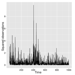
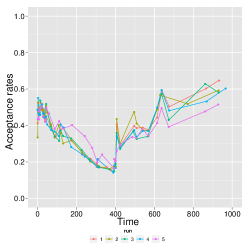
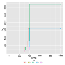
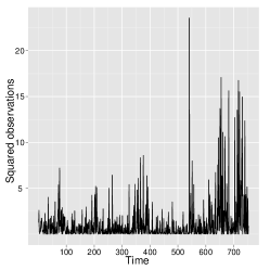
We applied the algorithm to a synthetic data set of length $T=1,000$ (Figure 1(a)) simulated with the values $\mu=0$, $\beta=0$, $\xi=0.5$, $\omega^{2}=0.0625$, $\lambda=0.01$ which were used also in the simulation study of Barndorff-Nielsen and Shephard, (2002). We launched 5 independent runs using $N_{\theta}=1,000$, a ESS threshold set at $50\%$, and the independent Hastings-Metropolis scheme described in Section 2.2. The number $N_{x}$ was set initially to 100, and increased whenever the acceptance rate went below $20\%$ (Figure 1(b)-(c)). Figure 1(d)-(e) shows estimates of the posterior marginal distribution of some parameters. Note the impact the large jump in the volatility has on $N_{x}$, which is systematically (across runs) increased around time $400$, and the posterior distribution of the parameters of the volatility process, see Figure 1(f).

Figure 1: Single-factor stochastic volatility model, synthetic dataset. (a) Squared observations vs time. (b)-(f) Results obtained from 5 repeated runs: (b) acceptance rate; (c) $N_{x}$ vs time; (d) to (f) overlaid kernel density estimators of the posterior distribution of $\mu$, $\beta$, $\xi$ at different times $t=250,500,1000$, the vertical dashed line indicates the true value and solid red lines the prior density.

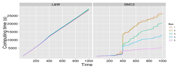
It is interesting to compare the numerical performance of SMC² to that of the SOPF and Liu and West, (2001)’s particle filter (referred to as L&W in the following) for this model and data, and for a comparable CPU budget. The SOPF, if run with $N=10^{5}$ particles, collapses to one single particle at about $t=700$ and is thus completely unusable in this context. L&W is a version of SOPF where the $\theta$-components of the particles are diversified using a Gaussian move that leaves the first two empirical moments of the particle sample unchanged. This move unfortunately introduces a bias which is hard to quantity. We implemented L&W with $N=2\times 10^{5}$ $(x,\theta)$-particles and we set the smoothing parameter $h$ to $10^{-1}$; see the Supplement for results with various values of $h$. This number of particles was to chosen to make the computing time of SMC² and L&W comparable, see Figure 2(a). Unsurprisingly, L&W runs are very consistent in terms of computing times, whereas those of SMC² are more variable, mainly because the number of $x$-particles does not reach the same value across the runs and the number of resample-move steps varies. Each of these runs took between $1.5$ and $7$ hours using a simple Python script and only one processing unit of a 2008 desktop computer (equipped with an Intel Core 2 Duo E8400). Note that, given that these methods could easily be parallelized, the computational cost can be greatly reduced; a $100\times$ speed-up is plausible using appropriate hardware.

Our results suggest that the bias in L&W is significant. Figure 2(b) shows the posterior distribution of $\xi$, the mean of volatility, at time $t=500$, which is about $100$ time steps after the large jump in volatility at time $t=407$. The results for both algorithms are compared to those from a long PMCMC run (implemented as in Peters et al.,, 2010, and detailed in the Supplement) with $N_{x}=500$ and $10^{5}$ iterations. Figure 2(c) reports on the estimation of the log evidence $\log p(y_{1:t})$ for each algorithm, plotting the estimated log evidence of each run minus the mean of the log evidence of the $5$ SMC² runs. We see that the log evidence estimated using L&W is systematically biased, positively or negatively depending on the time steps, with a large discontinuity at time $t=407$, which is due to underestimation of the tails of the predictive distribution.

Figure 2: Single-factor stochastic volatility model, synthetic dataset, comparison between methods. (a) Computing time of $5$ independent runs of L&W (left) and SMC² (right) in seconds, against time. (b) Estimation of the posterior marginal distribution of mean volatility, $\xi$. (c) Estimation of the log evidence, the curves represent the estimated evidence of each run minus the mean across $5$ runs of the log evidence estimated using SMC².

We now consider models of different complexity for the S&P 500 index. The data set is made of $753$ observations from January 3rd 2005 to December 31st 2007 and it is shown on Figure 3(a).

Figure 3: (a): the squares of the S&P 500 data from 03/01/2005 to 21/12/2007. (b): acceptance rates of the resample-move step for the full model over two independent runs. (c): log-evidence comparison between models (relative to the one-factor model).

We first consider a two-factor model, according to which the actual volatility is a sum of two independent components each of which follows a Lévy driven model. Previous research indicates that a two-factor model is sufficiently flexible, whereas more factors do not add significantly when considering daily data, see for example Barndorff-Nielsen and Shephard, (2002); Griffin and Steel, (2006) for Lévy driven models and Chernov et al., (2003) for diffusion-driven SV models. We consider one component which describes long-term movements in the volatility, with memory parameter $\lambda_{1}$, and another which captures short-term variation, with parameter $\lambda_{2}>>\lambda_{1}$. The second component allows more freedom in modelling the tails of the distribution of log-returns. The contribution of the slowly mixing process to the overall mean and variance of the spot volatility is controlled by the parameter $w\in(0,1)$. Thus, for this model $x_{t}=(v_{1,t},z_{1,t},v_{2,t},z_{2,t})$ with $v_{t}=v_{1,t}+v_{2,t}$, where each pair $(v_{i,t},z_{i,t})$ evolves according to (14) with parameters $(w_{i}\xi,w_{i}\omega^{2},\lambda_{i})$ with $w_{1}=w,w_{2}=1-w$. The system errors are generated by independent sets of variables $(k_{i},c_{i,1:k},e_{i,1:k})$, and $z_{0,i}$ are initialized according to the corresponding gamma distributions. Finally, we extend the observation equation to capture a significant feature observed in returns on stocks: low returns provoke increase in subsequent volatility, see for example Black, (1976) for an early reference. In parameter driven SV models, one generic strategy to incorporate such feedback is to correlate the noise in the observation and state processes, see Harvey and Shephard, (1996) in the context of the logarithmic SV model, and Section 3 of Barndorff-Nielsen and Shephard, (2001) for Lévy driven models. We take up their suggestion, and re-write the observation equation as

$$y_{t}=\mu+\beta v_{t}+v_{t}^{1/2}\epsilon_{t}+\rho_{1}\sum_{j=1}^{k_{1}}e_{1,j}+\rho_{2}\sum_{j=1}^{k_{2}}e_{2,j}-\xi(w\rho_{1}\lambda_{1}+(1-w)\rho_{2}\lambda_{2})$$ (15)

where $e_{i,j}$ are the system error variables involved in the generation of $v_{t}$ and $\rho_{i}$ are the leverage parameters which we expect to be negative. Thus, in this specification we deal with a model with a 5-dimensional state and 9 parameters.

The mathematical tractability of this family of models and the specification in terms of stationary and memory parameters allows to a certain extent subjective Bayesian modelling. Nevertheless, since the main emphasis here is to evaluate the performance of SMC² we choose priors that (as we verify a posteriori) are rather flat in the areas of high posterior density. Note that the prior for $\xi$ and $\omega^{2}$ has to reflect the scaling of the log-returns by a multiplicative factor. We take an $\mathrm{Exp}(1)$ prior for $\lambda_{1}$, an $\mathrm{Exp}(0.5)$ for $\lambda_{2}-\lambda_{1}$, thus imposing the identifiability constraint $\lambda_{2}>\lambda_{1}$. We take a $\mathrm{U}(0,1)$ prior for $w$, an $\mathrm{Exp}(1/5)$ for $\xi$ and $\omega^{2}$, and Gaussian priors with large variances for the observation equation parameters.

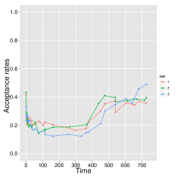
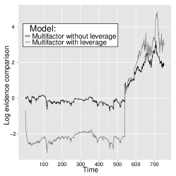
We launch the three models for the S&P 500 data: single factor, multifactor without and with leverage; note that multifactor without leverage means the full model, but with $\rho_{1}=\rho_{2}=0$ in (15). We use $N_{\theta}=2000$, and $N_{x}$ is set initially to $100$ and then dynamically increases as already described. The acceptance rates stay reasonable as illustrated on Figure 3. Figure 3 shows the log evidence $\log p(y_{1:t})$ for the two factor models minus the log evidence for the single factor model. Negative values at time $t$ means that the observations favour the single factor model up to time $t$. Notice how the model evidence changes after the big jump in volatility around time $t=550$. Estimated posterior densities for all parameters are provided in the Supplement.

4.2 Assessing extreme athletic records

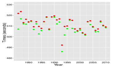
The second application illustrates the potential of SMC² in smoothing while accounting for parameter uncertainty. In particular, we consider state-space models that have been proposed for the dynamic evolution of athletic records, see for example Robinson and Tawn, (1995), Gaetan and Grigoletto, (2004), Fearnhead et al., 2010b . We analyse the time series of the best times recorded for women’s 3000 metres running events between 1976 and 2010. The motivation is to assess to which extent Wang Junxia’s world record in 1993 was unusual: $486.11$ seconds while the previous record was $502.62$ seconds. The data is shown in Figure 4 and include two observations per year $y=y_{1:2}$, with $y_{1}<y_{2}$: $y_{1}$ is the best annual time and $y_{2}$ the second best time on the race where $y_{1}$ was recorded. The data is available from http://www.alltime-athletics.com/ and it is further discussed in the aforementioned articles. A further fact that sheds doubt on the record is that the second time for 1993 corresponds to an athlete from the same team as the record holder.

We use the same modelling as Fearnhead et al., 2010b . The observations follow a generalized extreme value (GEV) distribution for minima, with cumulative distribution function $G$ defined by:

$$G(y|\mu,\xi,\sigma)=1-\exp\left[-\left\{1-\xi\left(\frac{y-\mu}{\sigma}\right)\right\}_{+}^{-1/\xi}\right]$$ (16)

where $\mu$, $\xi$ and $\sigma$ are respectively the location, shape and scale parameters, and $\{\cdot\}_{+}=\max(0,\cdot)$. We denote by $g$ the associated probability density function. The support of this distribution depends on the parameters; e.g. if $\xi<0$, $g$ and $G$ are non-zero for $y>\mu+\sigma/\xi$. The probability density function for $y=y_{1:2}$ is given by:

$$g(y_{1:2}|\mu,\xi,\sigma)=\{1-G(y_{2}|\mu,\xi,\sigma)\}\prod_{i=1}^{2}\frac{g(y_{i}|\mu,\xi,\sigma)}{1-G(y_{i}|\mu,\xi,\sigma)}\,$$ (17)

subject to $y_{1}<y_{2}$. The location $\mu$ is not treated as a parameter but as a smooth second-order random walk process:

$$x_{t}=(\mu_{t},\dot{\mu}_{t})^{\prime}\,,\quad x_{t+1}\mid x_{t},\nu\sim\mathcal{N}\left(Fx_{t},Q\right)\,,\quad F=\begin{pmatrix}1&1\\ 0&1\end{pmatrix}\text{ and }Q=\nu^{2}\begin{pmatrix}1/3&1/2\\ 1/2&1\end{pmatrix}$$ (18)

To complete the model specification we set a diffuse initial distribution $\mathcal{N}(520,10^{2})$ on $\mu_{0}$. Thus we deal with bivariate observations in time $y_{t}=y_{t,1:2}$, a state-space model with non-Gaussian observation density given in (17), a two-dimensional state process given in (18), and a $3$-dimensional unknown parameter vector, $\theta=(\nu,\xi,\sigma)$. We choose independent exponential prior distributions on $\nu$ and $\sigma$ with rate $0.2$. The sign of $\xi$ has determining impact on the support of the observation density, and the computation of extremal probabilities. For this application, given the form of (16) and the fact that the observations are necessarily bounded from below, it makes sense to assume that $\xi\leq 0$, hence we take an exponential prior distribution on $-\xi$ with rate $0.5$. (We also tried a $N(0,3^{2})$ prior, which had some moderate impact on the estimates presented below, but the corresponding results are not reported here.)

The data we will use in the analysis exclude the two times recorded on 1993. Thus, in an abuse of notation $y_{1976:2010}$ below refers to the pairs of times for all years but 1993, and in the model we assume that there was no observation for that year. Formally we want to estimate probabilities

$$p_{t}^{y}=\mathbb{P}(y_{t}\leq y|y_{1976:2010})=\int_{\Theta}\int_{\mathcal{X}}G(y|\mu_{t},\theta)p(\mu_{t}|y_{1976:2010},\theta)p(\theta|y_{1976:2010})\,d\mu_{t}d\theta$$

where the smoothing distribution $p(\mu_{t}|y_{1976:2010},\theta)$ and the posterior distribution $p(\theta|y_{1976:2010})$ appear explicitly; below we also consider the probabilities conditionally on the parameter values, rather than integrating over those. The interest lies in $p_{1993}^{486.11}$, $p_{1993}^{502.62}$ and $p_{t}^{cond}:=p_{t}^{486.11}/p_{t}^{502.62}$, which is the probability of observing at year $t$ Wang Junxia’s record given that we observe a better time than the previous world record. The rationale for using this conditional probability is to take into account the exceptional nature of any new world record.

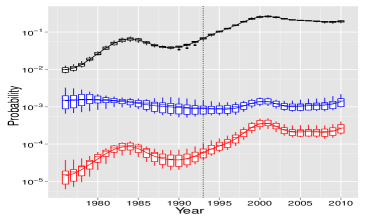
The algorithm is launched $10$ times with $N_{\theta}=1,000$ and $N_{x}=250$. The resample-move steps are triggered when the ESS goes below $50\%$, as in the previous example, and the proposal distribution used in the move steps is an independent Gaussian distribution fitted on the particles. The computing time of each of the $10$ runs varies between $30$ and $70$ seconds (using the same machine as in the previous section), which is why we allowed ourselves to use a fairly large number of particles compared to the small time horizon. Figure 4 represents the estimates $\hat{p}_{t}^{y}$ at each year, for $y=486.11$ (lower box-plots) and $y=502.62$ (upper box-plots), as well as $\hat{p}_{t}^{cond}=\hat{p}_{t}^{486.11}/\hat{p}_{t}^{502.62}$ (middle box-plots). The box-plots show the variability across the independent runs of the algorithm, and the lines connect the mean values computed across independent runs at each year. The mean value of $\hat{p}_{1993}^{cond}$ over the runs is $9.4\cdot 10^{-4}$ and the standard deviation over the runs is $3.3\cdot 10^{-4}$. Note that the estimates $\hat{p}_{t}^{y}$ are computed using the smoothing algorithm described in Section 3.3.

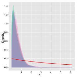
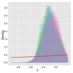
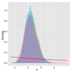
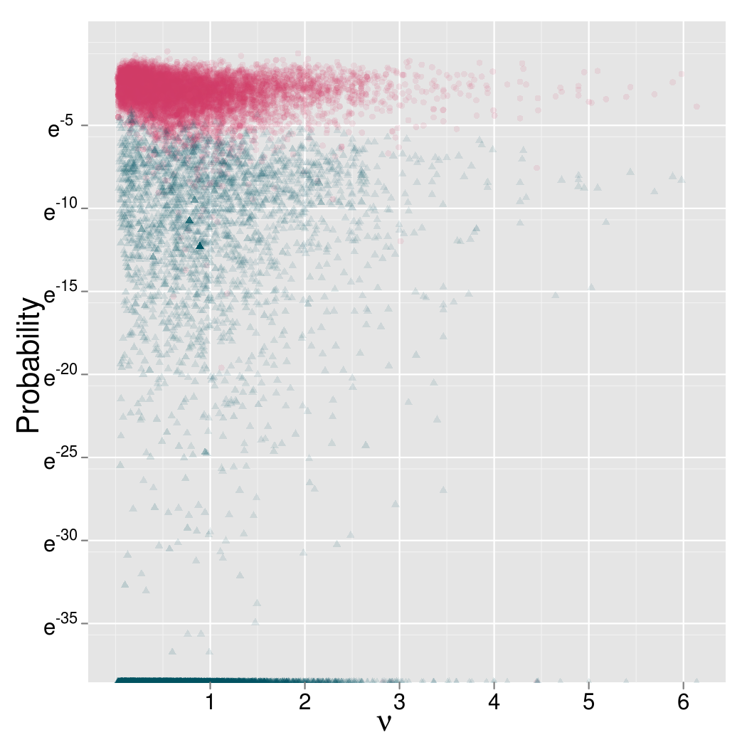
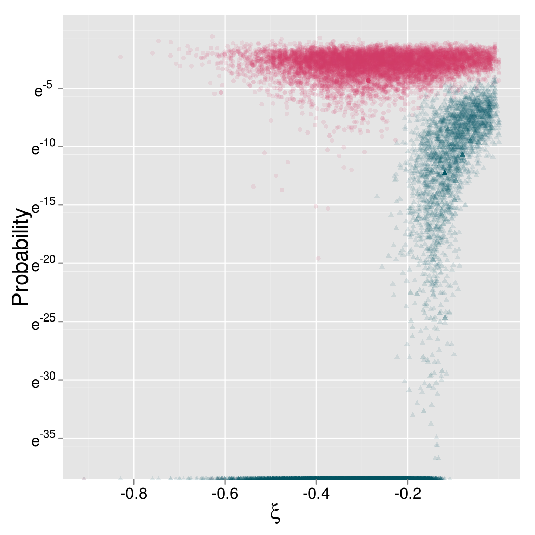
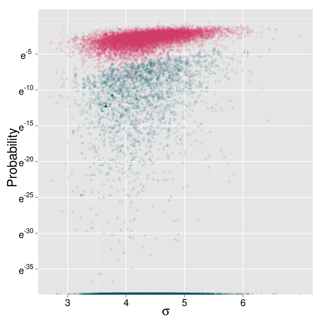
The second row of Figure 4 shows the posterior distributions of the three parameters $(\nu,\xi,\sigma)$ using kernel density estimations of the weighted $\theta$-particles. The density estimators obtained for each run are overlaid to show the consistency of the results over independent runs. The prior density function (full line) is nearly flat over the region of high posterior mass. The third row of Figure 4 shows scatter plots of the probabilities $G(y|\mu_{1993}^{n^{\star}(m)},\theta^{m})$ against the parameters $\theta^{m}$. The triangles represent these probabilities for $y=486.11$ while the circles represent the probabilities for $y=502.62$. The cloud of points at the bottom of these plots correspond to parameters $\theta^{m}$ for which the probability $G(486.11|\mu_{1993}^{n^{\star}(m)},\theta^{m})$ is exactly 0.

Figure 4: Athletics records. (a) Best two times of each year, in women’s 3000 metres events between 1976 and 2010; (b) box-plots over 10 runs of SMC² of estimates of the probability of interest (top) ${p_{t}^{502.62}}$, (middle) ${p_{t}^{cond}}$ and (bottom) ${p_{t}^{486.11}}$; the $y$-axis is in log scale and the dotted line indicates the year 1993; (c)-(e) posterior distribution of the parameters approximated by SMC², with results of $10$ independent runs overlaid on each plot and where the full line represents the prior density function; (f)-(h) probability of observing at year $1993$ a recorded time less than $486.11$ seconds (blue triangles, lower cloud of points) and less than $502.62$ seconds (red circles, upper cloud of points) against the components of $\theta$, where point sizes and transparencies are proportional to the weights of the $\theta$-particles.

5 Extensions

In this paper, we developed an “exact approximation” of the IBIS algorithm, that is, an ideal SMC algorithm targetting the sequence $\pi_{t}(\theta)=p(\theta|y_{1:t})$, with incremental weight $\pi_{t}(\theta)/\pi_{t-1}(\theta)=p(y_{t}|y_{1:t-1},\theta)$. The phrase “exact approximation”, borrowed from Andrieu et al., (2010), refers to the fact that our approach targets the exact marginal distributions, for any fixed value $N_{x}$.

5.1 Intractable densities

We have argued that SMC² can cope with state-space models with intractable transition densities provided these can be simulated from. More generally, it can cope with intractable transition of observation densities provided they can be unbiasedly estimated. Filtering for dynamic models with intractable densities for which unbiased estimators can be computed was discussed in Fearnhead et al., (2008). It was shown that replacing these densities by their unbiased estimators is equivalent to introducing additional auxiliary variables in the state-space model. SMC² can directly be applied in this context by replacing these terms by the unbiased estimators to obtain sequential state and parameter inference for such models.

5.2 SMC² for tempering

A natural question is whether we can construct other types of SMC² algorithms, which would be “exact approximations” of different SMC strategies. Consider for instance, again for a state-space model, the following geometric bridge sequence (in the spirit of e.g. Neal,, 2001), which allows for a smooth transition from the prior to the posterior:

$$\pi_{t}(\theta)\propto p(\theta)\left\{p(y_{1:T}|\theta)\right\}^{\gamma_{t}},\quad\gamma_{t}=t/L,$$

where $L$ is the total number of iterations. As pointed out by one referee, see also Fulop and Duan, (2011), it is possible to derive some sort of SMC² algorithm that targets iteratively the sequence

$$\pi_{t}(\theta)\propto p(\theta)\left\{\hat{p}(y_{1:T}|\theta)\right\}^{\gamma_{t}},\quad\gamma_{t}=t/L,$$

where $\hat{p}(y_{1:T}|\theta)$ is a particle filtering estimate of the likelihood. Note that $\left\{\hat{p}(y_{1:T}|\theta)\right\}^{\gamma_{t}}$ is not an unbiased estimate of $\left\{{p}(y_{1:T}|\theta)\right\}^{\gamma_{t}}$ when $\gamma_{t}\in(0,1)$. This makes the interpretation of the algorithm more difficult, as it cannot be analysed as a noisy, unbiased, version of an ideal algorithm. In particular, Proposition 2 on the complexity of SMC² cannot be easily extended to the tempering case. It is also less flexible in terms of PMCMC steps: for instance, it is not possible to implement the conditional SMC step described in Section 3.6.2, or more generally a particle Gibbs step, because such steps rely on the mixture representation of the target distribution, where the mixture index is some selected trajectory, see (9), and this representation does not hold in the tempering case. More importantly, this tempering strategy does not make it possible to perform sequential analysis as the SMC² algorithm discussed in this paper.

The fact remains that this tempering strategy may prove useful in certain non-sequential scenarios, as suggested by the numerical examples of Fulop and Duan, (2011). It may be used also for determining MAP (maximum a posteriori) estimators, and in particular the maximum likelihood estimator (using a flat prior), by letting $\gamma_{t}\rightarrow+\infty$.

Appendix A: Proof of Proposition (1)

We remark first that $\psi_{t,\theta}$ may be rewritten as follows:

$$\psi_{t,\theta}(x_{1:t}^{1:N_{x}},a_{1:t-1}^{1:N_{x}})=\left\{\prod_{n=1}^{N_{x}}q_{1,\theta}\left(x_{1}^{n}\right)\right\}\left\{\prod_{s=2}^{t}\prod_{n=1}^{N_{x}}W_{s-1,\theta}^{a_{s-1}^{n}}q_{s,\theta}\left(x_{s}^{n}|x_{s-1}^{a_{s-1}^{n}}\right)\right\}.$$

Starting from (7) and (3), one obtains

$$\pi_{t}(\theta,x_{1:t}^{1:N_{x}},a_{1:t-1}^{1:N_{x}}) = \frac{p(\theta)\psi_{t,\theta}(x_{1:t}^{1:N_{x}},a_{1:t-1}^{1:N_{x}})}{N_{x}^{t}p(y_{1:t})}\prod_{s=1}^{t}\left\{\sum_{n=1}^{N_{x}}w_{s,\theta}(x_{s-1}^{a_{s-1}^{n}},x_{s}^{n})\right\}$$

$$= \frac{p(\theta)}{N_{x}^{t}p(y_{1:t})}\sum_{n=1}^{N_{x}}\Bigg{[}w_{t,\theta}(x_{t-1}^{a_{t-1}^{n}},x_{t}^{n})\left\{\prod_{i=1}^{N_{x}}q_{1,\theta}(x_{1}^{i})\right\}$$

$$\qquad\left\{\prod_{s=2}^{t}\prod_{i=1}^{N_{x}}W_{s-1,\theta}^{a_{s-1}^{i}}q_{s,\theta}(x_{s}^{i}|x_{s-1}^{a_{s-1}^{i}})\right\}\prod_{s=1}^{t-1}\left\{\sum_{i=1}^{N_{x}}w_{s,\theta}(x_{s-1}^{a_{s-1}^{i}},x_{s}^{i})\right\}\Bigg{]}$$

by distributing the final product in the first line, and using the convention that $w_{1,\theta}(x_{0}^{a_{0}^{n}},x_{1}^{n})=w_{1,\theta}(x_{1}^{n})$.

To obtain (1), we consider the summand above, for a given value of $n$, and put aside the random variables that correspond to the state trajectory $\mathbf{x}_{1:t}^{n}$. We start with $\mathbf{x}_{1:t}^{n}(t)=x_{t}^{n}$, and note that

$$w_{t,\theta}(x_{t-1}^{a_{t-1}^{n}},x_{t}^{n})q_{t,\theta}(x_{t}^{n}|x_{t-1}^{a_{t-1}^{n}}) = f_{\theta}(x_{t}^{n}|x_{t-1}^{a_{t-1}^{n}})g_{\theta}(y_{t}|x_{t}^{n})$$

$$= f_{\theta}\left(\mathbf{x}_{1:t}^{n}(t)|\mathbf{x}_{1:t}^{n}(t-1)\right)g_{\theta}\left(y_{t}|\mathbf{x}_{1:t}^{n}(t)\right),$$

and that

$$W_{t-1,\theta}^{a_{t-1}^{n}}\left\{\sum_{i=1}^{N_{x}}w_{t-1,\theta}(x_{t-2}^{a_{t-2}^{i}},x_{t-1}^{i})\right\}=w_{t-1,\theta}\left(\mathbf{x}_{1:t}^{n}(t-2),\mathbf{x}_{1:t}^{n}(t-1)\right).$$

Thus, the summand in the expression of $\pi_{t}$ above may be rewritten as

$$w_{t-1,\theta}(\mathbf{x}_{1:t}^{n}(t-2),\mathbf{x}_{1:t}^{n}(t-1))f_{\theta}\left(\mathbf{x}_{1:t}^{n}(t)|\mathbf{x}_{1:t}^{n}(t-1)\right)g_{\theta}\left(y_{t}|\mathbf{x}_{1:t}^{n}(t)\right)\left\{\prod_{i=1}^{N_{x}}q_{1,\theta}(x_{1}^{i})\right\}\times\\ \left\{\prod_{s=2}^{t-1}\prod_{i=1}^{N_{x}}W_{s-1,\theta}^{a_{s-1}^{i}}q_{s,\theta}(x_{s}^{i}|x_{s-1}^{a_{s-1}^{i}})\right\}\left\{\prod_{\stackrel{{\scriptstyle i=1}}{{i\neq\mathbf{h}_{t}^{n}(n)}}}^{N_{x}}W_{t-1,\theta}^{a_{t-1}^{i}}q_{t,\theta}(x_{t}^{i}|x_{t-1}^{a_{t-1}^{i}})\right\}\prod_{s=2}^{t-1}\left\{\sum_{i=1}^{N_{x}}w_{s-1,\theta}(x_{s-2}^{a_{s-2}^{n}},x_{s-1}^{i})\right\}.$$

By applying recursively, for $s=t-1,\ldots,1$ the same type of substitutions, that is,

$$w_{s}\left(\mathbf{x}_{1:t}^{n}(s-1),\mathbf{x}_{1:t}^{n}(s)\right)q_{s,\theta}(x_{s}^{\mathbf{h}_{t}^{n}(s)}|x_{s-1}^{\mathbf{h}_{t}^{n}(s-1)}) = f_{\theta}\left(\mathbf{x}_{1:t}^{n}(s)|\mathbf{x}_{1:t}^{n}(s-1)\right)g_{\theta}\left(y_{s}|\mathbf{x}_{1:t}^{n}(s)\right),$$

$$w_{1}\left(\mathbf{x}_{1}^{n}(1)\right)q_{1,\theta}(x_{1}^{\mathbf{h}_{t}^{n}(1)}) = \mu_{\theta}\left(\mathbf{x}_{1:t}^{n}(1)\right)g_{\theta}\left(y_{1}|\mathbf{x}_{1:t}^{n}(1)\right),$$

and, for $s\geq 2$,

$$W_{s-1,\theta}^{a_{s-1}^{n}}\left\{\sum_{i=1}^{N_{x}}w_{s-1,\theta}(x_{s-2}^{a_{s-2}^{i}},x_{s-1}^{i})\right\}=w_{s-1,\theta}\left(\mathbf{x}_{1:t}^{n}(s-2),\mathbf{x}_{1:t}^{n}(s-1)\right).$$

and noting that

$$p(\theta,\mathbf{x}_{1:t}^{n},y_{1:t}) = p(y_{1:t})p(\theta|y_{1:t})p(\mathbf{x}_{1:t}^{n}|y_{1:t},\theta)$$

$$= p(\theta)\prod_{s=1}^{t}\left\{f_{\theta}\left(\mathbf{x}_{1:t}^{n}(s)|\mathbf{x}_{1:t}^{n}(s-1)\right)g_{\theta}\left(y_{s}|\mathbf{x}_{1:t}^{n}(s)\right)\right\},$$

where $p(\theta,\mathbf{x}_{1:t}^{n},y_{1:t})$ stands for the joint probability density defined by the model, for the triplet of random variables $(\theta,x_{1:t},y_{1:t})$, evaluated at $x_{1:t}=\mathbf{x}_{1:t}^{n}$, one eventually gets:

$$\pi_{t}(\theta,x_{1:t}^{1:N_{x}},a_{1:t-1}^{1:N_{x}})=p(\theta|y_{1:t})\times$$

$$\frac{1}{N_{x}^{t}}\sum_{n=1}^{N_{x}}p(\mathbf{x}_{1:t}^{n}|\theta,y_{1:t})\left\{\prod_{\begin{subarray}{c}i=1\\ i\neq\mathbf{h}_{t}^{n}(1)\end{subarray}}^{N_{x}}q_{1,\theta}(x_{1}^{i})\right\}\left\{\prod_{s=2}^{t}\prod_{\begin{subarray}{c}i=1\\ i\neq\mathbf{h}_{t}^{n}(s)\end{subarray}}^{N_{x}}W_{s-1,\theta}^{a_{s-1}^{i}}q_{s,\theta}(x_{s}^{i}|x_{s-1}^{a_{s-1}^{i}})\right\}.$$

Appendix B: Proof of Proposition 2 and discussion of assumptions

Since $p(\theta|y_{1:t})$ is the marginal distribution of $\bar{\pi}_{t,t+p}$, by iterated conditional expectation we get:

$$\frac{p(y_{t+1:t+p}|y_{1:t})^{2}}{\mathcal{E}_{t,t+p}^{N_{x}}} = \mathbb{E}_{p(\theta|y_{1:t})}\left[\mathbb{E}_{\bar{\pi}_{t,t+p}(\cdot|\theta)}\left\{\hat{Z}_{t+p|t}^{2}(\theta,x_{1:t+p}^{1:N_{x}},a_{1:t+p-1}^{1:N_{x}})\right\}\right]$$

$$= \mathbb{E}_{p(\theta|y_{1:t})}\left[\mathbb{E}_{\pi_{t}(\cdot|\theta)}\left\{\mathbb{E}_{\psi_{t+p|t}(\cdot|x_{1:t}^{1:N_{x}},a_{1:t-1}^{1:N_{x}}\theta)}\left\{\hat{Z}_{t+p|t}^{2}(\theta,x_{1:t+p}^{1:N_{x}},a_{1:t+p-1}^{1:N_{x}})\right\}\right\}\right]\,.$$

To study the inner expectation, we make the following first set of assumptions:

• For all $\theta\in\Theta$, and $x,x^{\prime},x^{\prime\prime}\in\mathcal{X}$,

  $$\frac{f_{\theta}(x|x^{\prime})}{f_{\theta}(x|x^{\prime\prime})}\leq\beta.$$

• For all $\theta\in\Theta$, $x,x^{\prime}\in\mathcal{X}$, $y\in\mathcal{Y}$,

  $$\frac{g_{\theta}(y|x)}{g_{\theta}(y|x^{\prime})}\leq\delta.$$

Under these assumptions, one obtains the following non-asymptotic bound.

Proposition 3 (Theorem 1.5 of Cérou et al., (2011))

For $N_{x}\geq\beta\delta p$,

$$\mathbb{E}_{\psi_{t+p|t}(\cdot|x_{1:t}^{1:N_{x}},a_{1:t-1}^{1:N_{x}}\theta)}\left\{\frac{\hat{Z}_{t+p|t}^{2}(\theta,x_{1:t+p}^{1:N_{x}},a_{1:t+p-1}^{1:N_{x}})}{p(y_{t+1:t+p}|y_{1:t},\theta)^{2}}\right\}-1\leq 4\beta\delta\frac{p}{N_{x}}.$$

The Proposition above is taken from Cérou et al., (2011), up to some change of notations and a minor modification: Cérou et al., (2011) establish this result for the likelihood estimate $\hat{Z}_{t}$, obtained by running a particle from time $1$ to time $t$. However, their proof applies straightforwardly to the partial likelihood estimate $\hat{Z}_{t+p|t}$, obtained by running a particle filter from time $t+1$ to time $t+p$, and therefore with initial distribution $\eta_{0}$ set to the mixture of Dirac masses at the particle locations at time $t$. We note in passing that Assumptions (H1a) and (H1b) may be loosened up slightly, see Whiteley, (2011). A direct consequence of Proposition 3, the main definitions and the iterated expectation is Proposition 2(a) for $\eta=4\beta\delta$.

Proposition 2(b) requires a second set of conditions taken from Chopin, (2002). These relate to the asymptotic behaviour of the marginal posterior distribution $p(\theta|y_{1:t})$ and they have been used to study the weight degeneracy of IBIS. Let $l_{t}(\theta)=\log p(y_{1:t}|\theta)$. The following assumptions hold almost surely.

• The MLE $\hat{\theta}_{t}$ (the mode of function $l_{t}(\theta)$) exists and converges to $\theta_{0}$ as $n\rightarrow+\infty$.

• The observed information matrix defined as

  $$\Sigma_{t}=-\frac{1}{t}\frac{\partial l_{t}(\hat{\theta}_{t})}{\partial\theta\partial\theta^{\prime}}$$

  is positive definite and converges to $I(\theta_{0})$, the Fisher information matrix.

• There exists $\Delta$ such that, for $\delta\in(0,\Delta)$,

  $$\limsup_{t\rightarrow+\infty}\left[\frac{1}{t}\sup_{\left\|\theta-\hat{\theta}_{t}\right\|>\delta}\left\{l_{t}(\theta)-l_{t}(\hat{\theta}_{t})\right\}\right]<0.$$

• The function $l_{t}/t$ is six-times continuously differentiable, and its derivatives of order six are bounded relative to $t$ over any compact set $\Theta^{\prime}\subset\Theta$.

Under these conditions one may apply Theorem 1 of Chopin, (2002) (see also Proof of Theorem 4 in Chopin,, 2004) to conclude that $\mathcal{E}_{t,t+p}^{\infty}\geq 2\gamma$ for a given $\gamma>0$ and $t$ large enough, provided $p=\left\lceil\tau t\right\rceil$ for some $\tau>0$ (that depends on $\gamma$). Together with Proposition 2(a) and by a small modification of the Proof of Theorem 4 in Chopin, (2004) to fix $\gamma$ instead of $\tau$, we obtain Proposition 2(b) provided $N_{x}=\lceil\eta t\rceil$, and $\eta=4\beta\delta$.

Note that (H2a) and (H2b) essentially amount to establishing that the MLE has a standard asymptotic behaviour (such as in the IID case). This type of results for state-space models is far from trivial, owning among other things to the intractable nature of the likelihood $p(y_{1:t}|\theta)$. A good entry in this field is Chapter 12 of Cappé et al., (2005), where it can be seen that the first set of conditions above, (H1a) and (H2b), are sufficient conditions for establishing (H2a) and (H2b), see in particular Theorem 12.5.7 page 465. Condition (H2d) is trivial to establish, if one assumes bounds similar to those in (H1a) and (H1b) for the derivatives of $g_{\theta}$ and $f_{\theta}$. Condition (H2c) is harder to establish. We managed to prove that this condition holds for a very simple linear Gaussian model; notes are available from the first author. Independent work by Judith Rousseau and Elisabeth Gassiat is currently carried out on the asymptotic properties of posterior distributions of state-space models, where (H2c) is established under general conditions (personal communication).

The implication of Proposition 2 to the stability of SMC² is based on the additional assumption that after resampling at time $t$ we obtain exact samples from $\pi_{t}$. In practice, this is only approximately true since an MCMC scheme is used to sample new particles. This assumption also underlies the analysis of IBIS in Chopin, (2002), where it was demonstrated empirically (see e.g. Fig. 1(a) in that paper) that the MCMC kernel which updates the $\theta$ particles has a stable efficiency over time since it uses the population of $\theta$-particles to design the proposal distribution. We also observe empirically that the performance of the PMCMC step does not deteriorate over time provided $N_{x}$ is increased appropriately, see for example Figure 1(b). It is important to establish such a result theoretically, i.e., that the total variation distance of the PMCMC kernel from the target distribution remains bounded over time provided $N_{x}$ is increased appropriately. Note that a fundamental difference between IBIS and SMC² is that respect is that in the latter the MCMC step targets distributions in increasing dimensions as time increases. Obtaining such a theoretical result is a research project on its own right, since such quantitative results lack, to the best of our knowledge, from the existing literature. The closest in spirit is Theorem 6 in Andrieu and Roberts, (2009) which, however, holds for “large enough” $N_{x}$, instead of providing a quantification of how large $N_{x}$ needs to be.

References

- Andrieu et al., (2010) Andrieu, C., Doucet, A., and Holenstein, R. (2010). Particle Markov chain Monte Carlo methods. J. R. Statist. Soc. B, 72(3):269–342.
- Andrieu and Roberts, (2009) Andrieu, C. and Roberts, G. (2009). The pseudo-marginal approach for efficient Monte Carlo computations. The Annals of Statistics, 37(2):697–725.
- Barndorff-Nielsen and Shephard, (2001) Barndorff-Nielsen, O. E. and Shephard, N. (2001). Non-Gaussian Ornstein-Uhlenbeck-based models and some of their uses in financial economics. J. R. Stat. Soc. Ser. B Stat. Methodol., 63(2):167–241.
- Barndorff-Nielsen and Shephard, (2002) Barndorff-Nielsen, O. E. and Shephard, N. (2002). Econometric analysis of realized volatility and its use in estimating stochastic volatility models. J. R. Stat. Soc. Ser. B Stat. Methodol., 64(2):253–280.
- Black, (1976) Black, F. (1976). Studies of stock price volatility changes. In Proceedings of the 1976 meetings of the business and economic statistics section, American Statistical Association, volume 177, page 81.
- Cappé et al., (2004) Cappé, O., Guillin, A., Marin, J. M., and Robert, C. (2004). Population Monte Carlo. J. Comput. Graph. Statist., 23:907–929.
- Cappé et al., (2005) Cappé, O., Moulines, E., and Rydén, T. (2005). Inference in Hidden Markov Models. Springer-Verlag, New York.
- Carpenter et al., (1999) Carpenter, J., Clifford, P., and Fearnhead, P. (1999). Improved particle filter for nonlinear problems. IEE Proc. Radar, Sonar Navigation, 146(1):2–7.
- Carvalho et al., (2010) Carvalho, C., Johannes, M., Lopes, H., and Polson, N. (2010). Particle learning and smoothing. Statistical Science, 25(1):88–106.
- Cérou et al., (2011) Cérou, F., Del Moral, P., and Guyader, A. (2011). A nonasymptotic theorem for unnormalized Feynman–Kac particle models. Ann. Inst. Henri Poincarré, 47(3):629–649.
- Chernov et al., (2003) Chernov, M., Ronald Gallant, A., Ghysels, E., and Tauchen, G. (2003). Alternative models for stock price dynamics. Journal of Econometrics, 116(1-2):225–257.
- Chopin, (2002) Chopin, N. (2002). A sequential particle filter for static models. Biometrika, 89:539–552.
- Chopin, (2004) Chopin, N. (2004). Central Limit Theorem for sequential Monte Carlo methods and its application to Bayesian inference. Ann. Stat., 32(6):2385–2411.
- Chopin, (2007) Chopin, N. (2007). Inference and model choice for sequentially ordered hidden Markov models. J. R. Statist. Soc. B, 69(2):269–284.
- Crisan and Doucet, (2002) Crisan, D. and Doucet, A. (2002). A survey of convergence results on particle filtering methods for practitioners. IEEE J. Sig. Proc., 50(3):736–746.
- Del Moral, (2004) Del Moral, P. (2004). Feynman-Kac Formulae. Springer.
- Del Moral et al., (2006) Del Moral, P., Doucet, A., and Jasra, A. (2006). Sequential Monte Carlo samplers. Journal of the Royal Statistical Society: Series B (Statistical Methodology), 68(3):411–436.
- Del Moral and Guionnet, (1999) Del Moral, P. and Guionnet, A. (1999). Central limit theorem for nonlinear filtering and interacting particle systems. Ann. Appl. Prob., 9:275–297.
- Douc and Moulines, (2008) Douc, R. and Moulines, E. (2008). Limit theorems for weighted samples with applications to sequential Monte Carlo methods. Ann. Statist., 36(5):2344–2376.
- Doucet et al., (2001) Doucet, A., de Freitas, N., and Gordon, N. J. (2001). Sequential Monte Carlo Methods in Practice. Springer-Verlag, New York.
- Doucet et al., (2000) Doucet, A., Godsill, S., and Andrieu, C. (2000). On sequential Monte Carlo sampling methods for Bayesian filtering. Statist. Comput., 10(3):197–208.
- Doucet et al., (2009) Doucet, A., Kantas, N., Singh, S., and Maciejowski, J. (2009). An overview of Sequential Monte Carlo methods for parameter estimation in general state-space models. In Proceedings IFAC System Identification (SySid) Meeting.
- Doucet et al., (2011) Doucet, A., Poyiadjis, G., and Singh, S. (2011). Sequential Monte Carlo computation of the score and observed information matrix in state-space models with application to parameter estimation. Biometrika, 98:65–80.
- Fearnhead, (2002) Fearnhead, P. (2002). MCMC, sufficient statistics and particle filters. Statist. Comput., 11:848–862.
- (25) Fearnhead, P., Papaspiliopoulos, O., Roberts, G., and Stuart, A. (2010a). Random weight particle filtering of continuous time processes. J. R. Stat. Soc. Ser. B Stat. Methodol., 72:497–513.
- Fearnhead et al., (2008) Fearnhead, P., Papaspiliopoulos, O., and Roberts, G. O. (2008). Particle filters for partially observed diffusions. J. R. Statist. Soc. B, 70:755–777.
- (27) Fearnhead, P., Wyncoll, D., and Tawn, J. (2010b). A sequential smoothing algorithm with linear computational cost. Biometrika, 97(2):447.
- Fulop and Duan, (2011) Fulop, A. and Duan, J. (2011). Marginalized sequential monte carlo samplers. Technical report, SSRN 1837772.
- Fulop and Li, (2011) Fulop, A. and Li, J. (2011). Robust and efficient learning: A marginalized resample-move approach. Technical report, SSRN 1724203.
- Gaetan and Grigoletto, (2004) Gaetan, C. and Grigoletto, M. (2004). Smoothing sample extremes with dynamic models. Extremes, 7(3):221–236.
- Gilks and Berzuini, (2001) Gilks, W. R. and Berzuini, C. (2001). Following a moving target - Monte Carlo inference for dynamic Bayesian models. J. R. Statist. Soc. B, 63:127–146.
- Gordon et al., (1993) Gordon, N. J., Salmond, D. J., and Smith, A. F. M. (1993). Novel approach to nonlinear/non-Gaussian Bayesian state estimation. IEE Proc. F, Comm., Radar, Signal Proc., 140(2):107–113.
- Griffin and Steel, (2006) Griffin, J. and Steel, M. (2006). Inference with non-Gaussian Ornstein-Uhlenbeck processes for stochastic volatility. Journal of Econometrics, 134(2):605–644.
- Harvey and Shephard, (1996) Harvey, A. and Shephard, N. (1996). Estimation of an asymmetric stochastic volatility model for asset returns. Journal of Business & Economic Statistics, 14(4):429–434.
- Jasra et al., (2007) Jasra, A., Stephens, D., and Holmes, C. (2007). On population-based simulation for static inference. Statistics and Computing, 17(3):263–279.
- Kim et al., (1998) Kim, S., Shephard, N., and Chib, S. (1998). Stochastic volatility: likelihood inference and comparison with ARCH models. Rev. Econ. Studies, 65(3):361–393.
- Kitagawa, (1998) Kitagawa, G. (1998). A self-organizing state-space model. J. Am. Statist. Assoc., 93:1203–1215.
- Koop and Potter, (2007) Koop, G. and Potter, S. M. (2007). Forecasting and estimating multiple change-point models with an unknown number of change-points. Review of Economic Studies, 74:763 – 789.
- Künsch, (2001) Künsch, H. (2001). State space and hidden Markov models. In Barndorff-Nielsen, O. E., Cox, D. R., and Klüppelberg, C., editors, Complex Stochastic Systems, pages 109–173. Chapman and Hall.
- Liu and Chen, (1998) Liu, J. and Chen, R. (1998). Sequential Monte Carlo methods for dynamic systems. J. Am. Statist. Assoc., 93:1032–1044.
- Liu and West, (2001) Liu, J. and West, M. (2001). Combined parameter and state estimation in simulation-based filtering. In Doucet, A., de Freitas, N., and Gordon, N. J., editors, Sequential Monte Carlo Methods in Practice, pages 197–223. Springer-Verlag.
- Liu, (2008) Liu, J. S. (2008). Monte Carlo strategies in scientific computing. Springer Series in Statistics. Springer, New York.
- Neal, (2001) Neal, R. M. (2001). Annealed importance sampling. Statist. Comput., 11:125–139.
- Oudjane and Rubenthaler, (2005) Oudjane, N. and Rubenthaler, S. (2005). Stability and uniform particle approximation of nonlinear filters in case of non ergodic signals. Stochastic Analysis and applications, 23:421–448.
- Papaspiliopoulos et al., (2007) Papaspiliopoulos, O., Roberts, G. O., and Sköld, M. (2007). A general framework for the parametrization of hierarchical models. Statist. Sci., 22(1):59–73.
- Peters et al., (2010) Peters, G., Hosack, G., and Hayes, K. (2010). Ecological non-linear state space model selection via adaptive particle markov chain monte carlo. Arxiv preprint arXiv:1005.2238.
- Roberts et al., (2004) Roberts, G. O., Papaspiliopoulos, O., and Dellaportas, P. (2004). Bayesian inference for non-Gaussian Ornstein-Uhlenbeck stochastic volatility processes. J. R. Stat. Soc. Ser. B Stat. Methodol., 66(2):369–393.
- Robinson and Tawn, (1995) Robinson, M. and Tawn, J. (1995). Statistics for exceptional athletics records. Applied Statistics, 44(4):499–511.
- Silva et al., (2009) Silva, R., Giordani, P., Kohn, R., and Pitt, M. (2009). Particle filtering within adaptive Metropolis Hastings sampling. Arxiv preprint arXiv:0911.0230.
- Storvik, (2002) Storvik, G. (2002). Particle filters for state-space models with the presence of unknown static parameters. IEEE Transaction on Signal Processing, 50:281–289.
- Whiteley, (2011) Whiteley, N. (2011). Stability properties of some particle filters. Arxiv preprint arXiv:1109.6779.