Estimators of Fractal Dimension: Assessing the Roughness of Time Series and Spatial Data

Abstract

The fractal or Hausdorff dimension is a measure of roughness (or smoothness) for time series and spatial data. The graph of a smooth, differentiable surface indexed in $\mathbb{R}^{d}$ has topological and fractal dimension $d$. If the surface is nondifferentiable and rough, the fractal dimension takes values between the topological dimension, $d$, and $d+1$. We review and assess estimators of fractal dimension by their large sample behavior under infill asymptotics, in extensive finite sample simulation studies, and in a data example on arctic sea-ice profiles. For time series or line transect data, box-count, Hall–Wood, semi-periodogram, discrete cosine transform and wavelet estimators are studied along with variation estimators with power indices 2 (variogram) and 1 (madogram), all implemented in the R package fractaldim. Considering both efficiency and robustness, we recommend the use of the madogram estimator, which can be interpreted as a statistically more efficient version of the Hall–Wood estimator. For two-dimensional lattice data, we propose robust transect estimators that use the median of variation estimates along rows and columns. Generally, the link between power variations of index $p>0$ for stochastic processes, and the Hausdorff dimension of their sample paths, appears to be particularly robust and inclusive when $p=1$.

keywordwidth330pt

, and T. Gneiting, H. Sevcikova, D. B. Percival

1 Introduction

Fractal-based analyses of time series, transects, and natural or man-made surfaces have found extensive applications in almost all scientific disciplines (Mandelbrot, 1982). While much of the literature ties fractal properties to statistical self-similarity, no such link is necessary. Rather, we adopt the argument of Bruno and Raspa (1989), Davies and Hall (1999) and Gneiting and Schlather (2004) that the fractal or Hausdorff dimension quantifies the roughness or smoothness of time series and spatial data in the limit as the observational scale becomes infinitesimally fine. In practice, measurements can only be taken at a finite range of scales, and usable estimates of the fractal dimension depend on the availability of observations at sufficiently fine temporal or spatial resolution (Malcai et al., 1997; Halley et al., 2004).

We follow common practice in defining the fractal dimension of a point set $X\subset\mathbb{R}^{d}$ to be the classical Hausdorff dimension (Hausdorff, 1919; Falconer, 1990). For $\varepsilon>0$, an $\varepsilon$-cover of $X$ is a finite or countable collection $\{B_{i}\dvtx i=1,2,\ldots\}$ of balls $B_{i}\subset\mathbb{R}^{d}$ of diameter $|B_{i}|$ less than or equal to $\varepsilon$ that covers $X$. With

$$H^{\delta}(X) = \lim_{\varepsilon\to 0}\inf\Biggl{\{}\sum_{i=1}^{\infty}|B_{i}|^{\delta}\dvtx\{B_{i}\dvtx i=1,2,\ldots\}$$

$$\hskip 77.0pt\mbox{is an $\varepsilon$-cover of }X\Biggr{\}}$$

denoting the $\delta$-dimensional Hausdorff measure of $X$, there exists a unique nonnegative value $D$ such that $H^{\delta}(X)=\infty$ if $\delta<D$ and $H^{\delta}(X)=0$ if $\delta>D$. This value $D$ is the Hausdorff dimension of the point set $X$. Under weak regularity conditions, the Hausdorff dimension coincides with the box-count dimension,

$$D_{\rm BC}=\lim_{\varepsilon\to 0}\frac{\log N(\varepsilon)}{\log(1/\varepsilon)},$$ (1)

where $N(\varepsilon)$ denotes the smallest number of cubes of width $\varepsilon$ in $\mathbb{R}^{d}$ which can cover $X$, and also with other natural and/or time-honored notions of dimension (Falconer, 1990).

=350pt Class Variogram or covariance Parameters Fractional Brownian motion $\gamma_{2}(t)=|c\hskip 0.85358ptt|^{\alpha}$ $\alpha\in(0,2]$ Matérn $\sigma(t)=\frac{2^{(\alpha/2)-1}}{\Gamma(\alpha/2)}|ct|^{\alpha/2}K_{\alpha/2}(|ct|)$ $\alpha\in(0,2]$ Powered exponential $\sigma(t)=\exp(-|ct|^{\alpha})$ $\alpha\in(0,2]$ Cauchy $\sigma(t)=(1+|ct|^{\alpha})^{-\tau/\alpha}$ $\alpha\in(0,2];\tau>0$ Dagum $\sigma(t)=1-(\frac{|ct|^{\tau}}{1+|ct|^{\tau}})^{\alpha/\tau}$ $\tau\in(0,2];\alpha\in(0,\tau)$

Table 1: Some parametric classes of variograms and covariance functions for a Gaussian process $\{X_{t}\dvtx t\in\mathbb{R}^{d}\}$. The covariance functions have been normalized such that $\sigma(0)=1$. Here, $\alpha$ is the fractal index, $c>0$ is a range parameter, and $K_{\nu}$ is a modified Bessel function of the second kind of order $\nu$. The Matérn and Dagum families allow for less restrictive assumptions on the parameters than stated here

In this paper we restrict attention to the case in which the point set

$$X=\{(t,X_{t})\in\mathbb{R}^{d}\times\mathbb{R}\dvtx t\in{\mathrm{T}}\subset\mathbb{R}^{d}\}\subset\mathbb{R}^{d+1}$$

is the graph of time series or spatial data observed at a finite set ${\mathrm{T}}\subset\mathbb{R}^{d}$ of typically regularly spaced times or locations. The fractal dimension then refers to the properties of the curve ($d=1$) or surface ($d\geq 2$) that arises in the continuum limit as the data are observed at an infinitesimally dense subset of the temporal or spatial domain, which without loss of generality can be assumed to be the unit interval or unit cube. In time series analysis and spatial statistics, this limiting scenario is referred to as infill asymptotics (Hall and Wood, 1993; Dahlhaus, 1997; Stein, 1999).

If the limit curve or limit surface is smooth and differentiable, its fractal dimension, $D$, equals its topological dimension, $d$. For a rough and nondifferentiable curve or surface, the fractal dimension may exceed the topological dimension. For example, suppose that $\{X_{t}\dvtx t\in\mathbb{R}^{d}\}$ is a Gaussian process with stationary increments, whose variogram or structure function,

$$\gamma_{2}(t)=\tfrac{1}{2}{\mathbb{E}}(X_{u}-X_{u+t})^{2},$$ (2)

satisfies

$$\gamma_{2}(t)=|c_{2}t|^{\alpha}+\mathcal{O}(|t|^{\alpha+\beta})\quad\mbox{as }t\to 0,$$ (3)

where $\alpha\in(0,2]$, $\beta\geq 0$, and $c_{2}>0$, and $|\cdot|$ denotes the Euclidean norm. Then the graph of a sample path has fractal dimension

$$D=d+1-\frac{\alpha}{2}$$ (4)

almost surely (Orey, 1970; Adler 1981). This relationship links the fractal dimension of the sample paths to the behavior of the variogram or structure function at the coordinate origin, and can be extended to broad classes of potentially anisotropic and nonstationary processes, as well as some non-Gaussian processes (Adler, 1981; Hall and Roy, 1994; Xue and Xiao, 2011). It allows us to think of fractal dimension as a second-order property of a Gaussian stochastic process, in addition to being a roughness measure for a realized curve or surface. Accordingly, we refer to the index $\alpha$ in the asymptotic relationship (3) as the fractal index.

Table 1 provides examples of Gaussian processes that exhibit this asymptotic behavior. FractionalBrownian motion is a nonstationary, statistically self-similar process that is defined in terms of the variogram (Mandelbrot and Van Ness, 1968). The other entries in the table refer to stationary processes with covariance function $\sigma(t)={\rm cov}(X_{u},X_{t+u})$, which relates to the variogram as

$$\gamma_{2}(t)=\sigma(0)-\sigma(t),\quad t\in\mathbb{R}^{d}.$$

Key examples include the Matérn family (Matérn, 1986; Guttorp and Gneiting, 2006), used by Goff and Jordan (1988) to parameterize the fractal dimension of oceanic features; the Cauchy class, introduced by Gneiting and Schlather (2004) to illustrate local and global properties of random functions; and the Dagum family (Berg, Mateu and Porcu, 2008). In simulation settings, the powered exponential class (Yaglom, 1987) is a convenient default example. The exponent $\beta$ in the asymptotic relationship (3) equals $\beta=2-\alpha$ for the Matérn class, $\beta=\alpha$ for the powered exponential and Cauchy families, and $\beta=\tau$ for the Dagum family. Generally, the smaller the value of $\beta$, the harder the estimation of the fractal index, $\alpha$, and the more pronounced the finite sample bias of estimators of the fractal index or fractal dimension.

Figure 1: Sample paths of stationary Gaussian processes with powered exponential covariance function, $\sigma(t)=\exp(-|t|^{\alpha})$, and fractal index, $\alpha$, equal to 1.9, 1.4, 1.0 and 0.2. The corresponding values of the fractal dimension, $D$, are 1.05, 1.3, 1.5 and 1.9, respectively. The simulation domain is a grid over the unit interval with spacing $1/1{,}024$.

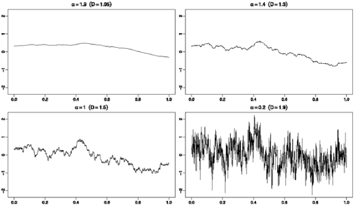
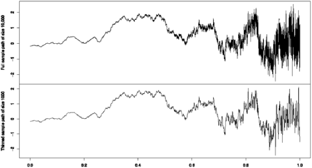
As an illustration for time series or line transect data, Figure 1 displays Gaussian sample paths from the powered exponential family with the fractal index, $\alpha$, ranging from 1.9 to 0.2, and the fractal dimension, $D$, extending from 1.05 to 1.9. The smaller $\alpha$, the rougher the sample path, and the larger the fractal dimension, with the lower limit, $D=1$, being associated with a smooth curve, and the upper limit, $D=2$, corresponding to a space-filling, exceedingly rough graph. Figure 2 shows a realization from the nonstationary Gaussian Matérn model of Anderes and Stein (2011), in a case in which the fractal index and the fractal dimension vary linearly along the unit interval. To illustrate the visual effects of the measurement scale, both the original sample path of size 10,000 and an equidistantly thinned version of size 1,000 are shown.

Figure 2: A sample path from the nonstationary Gaussian Matérn process of Anderes and Stein (2011), where the fractal dimension, $D$, grows linearly from $D=1$ at time $t=0$ to $D=2$ at time $t=1$. To illustrate the visual effects of the temporal resolution, both the original sample path with grid spacing $1/10{,}000$ (top panel) and an equidistantly thinned version with grid spacing $1/1{,}000$ (bottom panel) are shown. The nonstationary covariance is given by equation (10) of Anderes and Stein (2011) with $\sigma^{2}=1$, $\rho=1/2$, and linearly varying local smoothness parameter, $\nu_{t}=1-t$.

Figure 3: Sample surfaces of stationary spatial Gaussian processes with the powered exponential covariance function, $\sigma(t)=\exp(-|t|^{\alpha})$, and fractal index, $\alpha$, equal to 1.5, 1.0 and 0.2. The corresponding values of the fractal dimension, $D$, are 2.25, 2.5 and 2.9. The simulation domain is a grid on the unit square in $\mathbb{R}^{2}$ with spacing $1/512$ along each coordinate.

Turning to spatial data, Figure 3 shows Gaussian sample surfaces from the powered exponential class with the fractal index, $\alpha$, being equal to 1.5, 1.0 and 0.2. The surfaces are increasingly rough with the fractal dimension, $D$, being equal to 2.25, 2.5 and 2.9, respectively.

A wealth of applications requires the characterization of the roughness or smoothness of time series, line transect or spatial data, with Burrough (1981) and Malcai et al. (1997) summarizing an impressive range of experimental results. For example, fractal dimensions have been studied for geographic profiles and surfaces, such as the underside of sea ice (Rothrock and Thorndike, 1980), the topography of the sea floor (Goff and Jordan, 1988), Martial surface (Orosei et al., 2003) and terrestrial features (Weissel, Pratson and Malinverno, 1994; Turcotte, 1997; Gagnon, Lovejoy and Schertzer, 2006). Further references can be found in Molz, Rajaram and Lu (2004) for applications in subsurface hydrology and in Halley et al. (2004) for applications in ecology. Not surprisingly then, estimators for the fractal dimension have been proposed and widely used in various literatures, including physics, engineering, the earth sciences, and statistics, with the works of Burrough (1981), Goff and Jordan (1988), Bruno and Raspa (1989), Dubuc et al. (1989a, 1989b), Jakeman and Jordan (1990), Theiler (1990), Klinkenberg and Goodchild (1992), Schepers, van Beek and Bassingthwaighte (1992), Hall and Wood (1993), Constantine and Hall (1994), Kent and Wood (1997), Davies and Hall (1999), Chan and Wood (2000), Zhu and Stein (2002), Chan and Wood (2004) and Bez and Bertrand (2011) being examples. Our objectives in this paper are to survey the literature across disciplines, review and assess the various types of estimators, and provide recommendations for practitioners, along with novel directions for theoretical work.

The remainder of the paper is organized as follows. In Section 2 we describe estimators of fractal dimension for time series and line transect data, including box-count, Hall–Wood, variogram, madogram, power variation, semi-periodogram and wavelet-based techniques. Then in Section 3 we assess and compare the estimators. Considering both efficiency and robustness, we concur with Bruno and Raspa (1989) and Bez and Bertrand (2011) and recommend the use of the madogram estimator, that is, the variation estimator with power index $p=1$, which can be interpreted as a statistically efficient version of the Hall–Wood estimator. An underlying motivation is that for an intrinsically stationary process with variogram of order $p>0$ of the form

$$\quad\gamma_{p}(t) = \tfrac{1}{2}{\mathbb{E}}|X_{u}-X_{u+t}|^{p}$$

$$= |c_{p}t|^{\alpha p/2}+\mathcal{O}\bigl{(}|t|^{(\alpha+\beta)p/2}\bigr{)}\quad\mbox{as }t\to 0,$$

the relationship (4) between the fractal index, $\alpha$, and the fractal dimension, $D$, appears to be more robust and inclusive when $p=1$, as compared to the default case, in which $p=2$.

Section 4 discusses ways in which estimators for the time series or line transect case can be adapted to spatial data observed over a regular lattice in $\mathbb{R}^{2}$, and Section 5 evaluates these proposals. Our preferred estimators in this setting are simple, robust transect estimators that employ the median of variation estimates with power index $p=1$ along individual rows and columns. A data example on arctic sea-ice profiles is given in Section 6. The paper ends in Section 7, where we make a call for new directions in theoretical and methodological work that addresses both probabilists and statisticians. Furthermore, we hint at inference for nonstationary or multifractional processes, where the fractal dimension of a sample path may vary temporally or spatially. All computations in the paper use the fractaldim package (Ševčíková, Gneiting and Percival, 2011), which implements our proposals in R (Ihaka and Gentleman, 1996).

2 Estimating the Fractal Dimension of Time Series and Line Transect Data

Spurred and inspired by the now classical essay of Mandelbrot (1982), a large number of methods have been developed for estimating fractal dimension. By the early 1990s a sizable, mostly heuristic literature on the estimation of fractal dimension for time series and line transect data had accumulated in the physical, engineering and earth sciences, where various reviews are available (Dubuc et al., 1989a; Klinkenberg and Goodchild, 1992; Schepers, van Beek and Bassingthwaighte, 1992; Gallant et al., 1994; Klinkenberg, 1994; Schmittbuhl, Vilotte and Roux, 1995). These developments prompted the statistical community to introduce new methodology, along with asymptotic theory for box-count (Hall and Wood, 1993), variogram (Constantine and Hall, 1994; Kent and Wood, 1997), level crossing (Feuerverger, Hall and Wood, 1994) and spectral (Chan, Hall and Poskitt, 1995) estimators, among others.

Essentially all methods follow a common scheme, in that: [(a)]

a certain numerical property, say $Q$, of the time series or line transect data is computed as a function of “scale,” say $\varepsilon$;

an asymptotic power law $Q(\varepsilon)\propto\varepsilon^{b}$ as the scale $\varepsilon\to 0$ becomes infinitesimally small is derived or postulated; where

the scaling exponent, $b$, is a linear function of the fractal dimension, $D$;

and thus $D$ is estimated by linear regression of $\log Q(\varepsilon)$ on $\log\varepsilon$, with emphasis on the smallest observed values of the scale $\varepsilon$. Table 2 shows the data property, the measure of scale and the scaling law for various methods. For techniques working in the spectral domain, the scaling law applies as the frequency grows to infinity, equivalent to the scale becoming infinitesimally small in the time domain.

=380pt Method Property Scale Scaling law Regime Box-count $N(\varepsilon)$: number of boxes $\varepsilon$: box width $N(\varepsilon)\propto\varepsilon^{-D}$ $\varepsilon\to 0$ Divider $L(\varepsilon)$: length of curve $\varepsilon$: step size $L(\varepsilon)\propto\varepsilon^{-1-D}$ $\varepsilon\to 0$ Level crossing $M(h)$: number of crossings $h$: bandwidth $M(h)\propto h^{1-D}$ $h\to 0$ Variogram $\gamma_{2}(t)$: variogram $t$: lag $\gamma_{2}(t)\propto t^{4-2D}$ $t\to 0$ Madogram $\gamma_{1}(t)$: madogram $t$: lag $\gamma_{1}(t)\propto t^{2-D}$ $t\to 0$ Spectral $f(\omega)$: spectral density $\omega$: frequency $f(\omega)\propto\omega^{2D-5}$ $\omega\to\infty$ Wavelet $\nu^{2}(\tau)$: wavelet variance $\tau$: scale $\nu^{2}(\tau)\propto\tau^{4-2D}$ $\tau\to 0$

Table 2: Some extant methods for estimating the fractal dimension of time series and line transect data

In the balance of this section, we describe the most popular estimators of fractal dimension in the equally spaced time series or line transect setting. Without loss of generality, we may assume that the observation domain is the unit interval. In the case of $n_{s}=n+1$ equally spaced observations, the data graph is the point set

$$\biggl{\{}(t,X_{t})\dvtx t=\frac{i}{n},i=0,1,\ldots,n\biggr{\}}\subset\mathbb{R}^{2}.$$ (6)

The relevant asymptotic regime then is infill asymptotics, in which the number of observations grows to infinity, whereas the underlying domain, namely the unit interval, remains fixed. For convenience in what follows, we refer to both $n$ and $n_{s}$ as the sample size.

2.1 Box-Count Estimator

The popular box-count estimator is motivated by the scaling law (1) that defines the box-count dimension. The basic idea is simple, in that the time series graph is initially covered by a single box. The box is divided into four quadrants, and the number of cells required to cover the curve is counted. Then each subsequent quadrant is divided into four subquadrants, and one continues doing so until the box width equals the resolution of the data, keeping track of the number of quadrants required to cover the graph at each step. If $N(\varepsilon)$ denotes the number of boxes required at width or scale $\varepsilon$, the box-count estimator equals the slope in an ordinary least squares regression fit of $\log N(\varepsilon)$ on $\log\varepsilon$. Similarly to Mandelbrot’s (1967) divider technique, the method can be used to quantify the fractal dimension of any planar point set, rather than just equally spaced time series or line transect data.

Figure 4: Illustration of the box-count algorithm and naive box-count estimates for the two datasets in the lower row of Figure 1. See the text for details.

Figure 5: Log-log regression for the standard version of the box-count estimator and the datasets in the lower row of Figure 1. Only the points marked with filled circles are used when fitting the regression line.

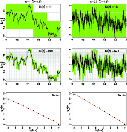
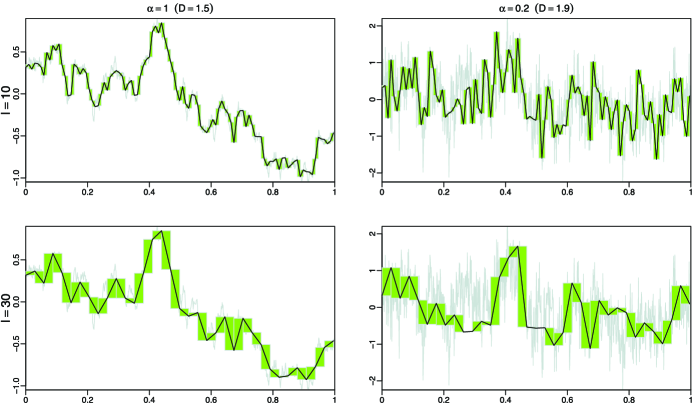
In our setting of a data graph of the form (6), where, for simplicity, we assume that $n=2^{K}$ is a power of 2, the box-count algorithm can be summarized as follows. Let $u=\max_{0\leq j\leq n}X_{j/n}-\min_{0\leq j\leq n}X_{j/n}$ denote the range of the data. Consider scales $\varepsilon_{k}=2^{k-K}$ where $k=0,1,\ldots,K$. At the largest scale, $\varepsilon_{K}=1$, the graph (6) can be covered by a single box of width $1$ and height $u$, which we now call the bounding box. At scale $\varepsilon_{k}$ the bounding box can be tiled by $4^{K-k}$ boxes of width $2^{k-K}$ and height $u2^{k-K}$ each, and we define $N(\varepsilon_{k})$ to be the number of such boxes that intersect the linearly interpolated data graph. Figure 4 provides an illustration on two of the datasets in Figure 1, for which $n=1024$ and $K=10$. For example, the upper left plot considers $k=8$, where $\varepsilon_{8}=2^{-2}$ and $N(\varepsilon_{8})=11$, and the middle left plot looks at $k=5$, where $\varepsilon_{5}=2^{-5}$ and $N(\varepsilon_{5})=207$. The naive box-count estimator then uses the slope in an ordinary least squares regression fit of $\log N(\varepsilon)$ on $\log\varepsilon$, that is,

$$\widehat{D}_{\mathrm{B}C}=-\Biggl{\{}\sum_{k=0}^{K}(s_{k}-\bar{s})\log N(\varepsilon_{k})\Biggr{\}}\Biggl{\{}\sum_{k=0}^{K}(s_{k}-\bar{s})^{2}\Biggr{\}}^{-1},$$

where $s_{k}=\log\varepsilon_{k}$ and $\bar{s}$ is the mean of $s_{0},s_{1},\ldots,s_{K}$. In our illustrating example, this leads to the estimates shown in the lower row of Figure 4.

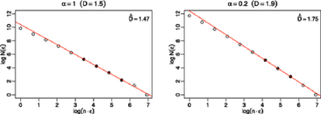
Several authors identified problems with the naive estimator that includes all scales in the regression fit of $\log N(\varepsilon)$ on $\log\varepsilon$, and proposed modifications that address these issues (Dubuc et al., 1989a; Liebovitch and Toth, 1989; Block, von Bloh and Schellnhuber, 1990; Taylor and Taylor, 1991). Indeed, one always has $N(\varepsilon_{0})\geq n$ and $N(\varepsilon_{K})=1$, which suggests that the counts at both the smallest and the largest scales ought to be discarded. Liebovitch and Toth (1989) proposed to exclude the smallest scales $\varepsilon_{k}$ for which $N(\varepsilon_{k})>n/5$, as well as the two largest scales, from the regression fit. We adopt this proposal in our standard version of the box-count estimator, as illustrated in Figure 5. The restriction on the scales improves the statistical and computational efficiency of the estimator. However, it is in the limit as $\varepsilon\to 0$ that the underlying scaling law (1) operates, and thus it is unfortunate that information at the very smallest scales is discarded.

A natural variant of the box-count estimator uses scales $\varepsilon_{l}=l/n$, rather than scales $\varepsilon_{k}=2^{k}/n$ at the powers of 2 only. In the next section we discuss a related estimator that takes up this idea, addresses the aforementioned limitations, and is tailored to time series data of the form (6).

Figure 6: Illustration of the Hall–Wood algorithm for the datasets in the lower row of Figure 1. The quantity $\widehat{A}(l/n)$ is computed as the sum of the colored areas, where $n=1{,}024$, $l=10$ (upper row) and $l=30$ (lower row).

2.2 Hall–Wood Estimator

Hall and Wood (1993) introduced a version of the box-count estimator that operates at the smallest observed scales and avoids the need for rules of thumb in its implementation.

To motivate their proposal, let $A(\varepsilon)$ denote the total area of the boxes at scale $\varepsilon$ that intersect with the linearly interpolated data graph (6). There are $N(\varepsilon)$ such boxes, and so $A(\varepsilon)\propto N(\varepsilon)\hskip 0.85358pt\varepsilon^{2}$, which leads us to a reformulation of definition (1), namely,

$$D_{\rm BC}=2-\lim_{\varepsilon\to 0}\frac{\log A(\varepsilon)}{\log(\varepsilon)}.$$ (7)

At scale $\varepsilon_{l}=l/n$, where $l=1,2,\ldots,$ an estimator of $A(l/n)$ is

$$\widehat{A}(l/n)=\frac{l}{n}\sum_{i=1}^{\lfloor n/\hskip 0.85358ptl\rfloor}\bigl{|}X_{il/n}-X_{(i-1)l/n}\bigr{|},$$ (8)

where $\lfloor n/l\rfloor$ denotes the integer part of $n/l$. Figure 6 suggests a natural interpretation of this quantity, in that it approximates $A(l/n)$, with all features at scales less than $l/n$ being ignored. For an alternative, and potentially preferable, interpretation in terms of power variations, see Section 2.4.

Figure 7: Log–log regression for the Hall–Wood estimator (10) and the datasets in the lower row of Figure 1. Only the two points marked with filled circles are used when fitting the regression line.

Figure 8: Log-log regression for the variogram estimator (13) and the datasets in the lower row of Figure 1. Only the two points marked with filled circles are used when fitting the regression line.

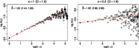
The Hall–Wood estimator with design parameter $m=1$, as used in the numerical experiments of Hall and Wood (1993), is based on an ordinary least squares regression fit of $\log\widehat{A}(l/n)$ on $\log(l/n)$:

$$\widehat{D}_{\mathrm{HW}}=2-\Biggl{\{}\sum_{l=1}^{L}(s_{l}-\bar{s})\log\widehat{A}(l/n)\Biggr{\}}\Biggl{\{}\sum_{l=1}^{L}(s_{l}-\bar{s})^{2}\Biggr{\}}^{-1},$$ (9)

where $L\geq 2$, $s_{l}=\log(l/n)$ and $\bar{s}=\frac{1}{L}\sum_{l=1}^{L}s_{l}$. Hall and Wood (1993) recommended the use of $L=2$ to minimize bias, which is unsurprising, in view of the limit in (7) being taken as $\varepsilon\to 0$. Using $L=2$ yields our standard implementation of the Hall–Wood estimator, namely,

$$\widehat{D}_{\mathrm{HW}}=2-\frac{\log\widehat{A}(2/n)-\log\widehat{A}(1/n)}{\log 2}.$$ (10)

Figure 7 shows the corresponding log–log plots and regression fits in our illustrating example.

2.3 Variogram Estimator

Owing to its intuitive appeal and ease of implementation, the variogram estimator has been very popular. A prominent early application is that of Burrough (1981). The first asymptotic study under the infill scenario was published in the physics literature (Jakeman and Jordan, 1990), followed by key contributions of Constantine and Hall (1994), Kent and Wood (1997), Davies and Hall (1999) and Chan and Wood (2004) in statistical journals.

Recall that the variogram or structure function $\gamma(t)$ of a stochastic process $\{X_{t}\dvtx t\in\mathbb{R}\}$ with stationary increments is defined in (2) as one-half times the expectation of the square of an increment at lag $t$. The classical method of moments estimator for $\gamma(t)$ at lag $t=l/n$ from time series or line transect data (6) is

$$\quad\widehat{V}_{2}(l/n)=\frac{1}{2(n-l)}\sum_{i=l}^{n}\bigl{(}X_{i/n}-X_{(i-l)/n}\bigr{)}^{2}.$$ (11)

In view of the relationship (4) between the fractal index, defined in (3), and the fractal dimension, $D$, a regression fit of $\log\widehat{V}(t)$ on $\log t$ yields the variogram estimator,

$$\widehat{D}_{{\mathrm{V}};2} = 2-\frac{1}{2}\Biggl{\{}\sum_{l=1}^{L}(s_{l}-\bar{s})\log\widehat{V}_{2}(l/n)\Biggr{\}}$$

$${}\hskip 15.0pt\cdot\Biggl{\{}\sum_{l=1}^{L}(s_{l}-\bar{s})^{2}\Biggr{\}}^{-1},$$

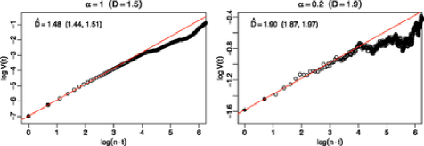
where $L\geq 2$, $s_{l}=\log(l/n)$ and $\bar{s}$ is the mean of $s_{1},\ldots,s_{L}$. Figure 8 illustrates the log–log regression for the datasets in the lower row of Figure 1. In addition to the corresponding point estimate, we provide a 90% central interval estimate, using the parametric bootstrap method as proposed by Davies and Hall (1999).

Constantine and Hall (1994) argued that the bias of the variogram estimator increases with the cut-off $L$ in the log–log regression, and Davies and Hall (1999) showed numerically that the mean squared error (MSE) of the estimator for a Gaussian process with powered exponential covariance is minimized when $L=2$. Zhu and Stein (2002) argued similarly in a spatial setting. These results are unsurprising and have intuitive support from the fact that the behavior of the theoretical variogram in an infinitesimal neighborhood of zero determines the fractal dimension of the Gaussian sample paths. We thus choose $L=2$ in our implementation, resulting in the estimate

$$\quad\widehat{D}_{{\mathrm{V}};2}=2-\frac{1}{2}\frac{\log\widehat{V}_{2}(2/n)-\log\widehat{V}_{2}(1/n)}{\log 2}.$$ (13)

As Kent and Wood (1997) suggested, generalized least squares rather than ordinary least squares regression could be employed, though the methods coincide when $L=2$.

It is well known that the method of moments estimator (11) is nonrobust. It is therefore tempting to replace it by the highly robust variogram estimator proposed by Genton (1998), which is based on the robust estimator of scale of Rousseeuw and Croux (1993). We implemented an estimator of the fractal dimension that uses (2.3) with $L=2$, but with the method of moments estimate (11) replaced by Genton’s highly robust variogram estimator. In a simulation setting, this estimator works well. However, it breaks down frequently when applied to real data, where it yields very limited, discrete sets of possible values for the estimate only. Upon further investigation, this stems from the ubiquitous discreteness of real-world data, under which the Rousseeuw and Croux (1993) estimator can fail, in ways just described. While discreteness is a general issue when estimating fractal dimension, the problem is exacerbated by the use of this estimator. In this light, the next section investigates another approach to more robust estimators of fractal dimension.

2.4 Variation Estimators

We now discuss a generalization of the variogram estimator that is based on the variogram of order $p$ of a stochastic process with stationary increments, namely,

$$\gamma_{p}(t)=\tfrac{1}{2}{\mathbb{E}}|X_{u}-X_{t+u}|^{p}.$$ (14)

When $p=2$, we recover the variogram (2), when $p=1$ the madogram, and when $p=1/2$ the rodogram (Bruno and Raspa, 1989; Emery, 2005; Bez and Bertrand 2011). Standard arguments show that a Gaussian process with a variogram of the form (3) admits analogous expansions of the variogram of order $p$, in that

$$\ \gamma_{p}(t)=|c_{p}t|^{\alpha p/2}+\mathcal{O}\bigl{(}|t|^{(\alpha+\beta)p/2}\bigr{)}\quad\mbox{as }t\to 0,$$ (15)

with fixed values of the fractal index, $\alpha\in(0,2]$,$\beta>0$, and a constant $c_{p}>0$ that satisfies

$$c_{p}=\biggl{(}\frac{2^{p-1}}{\sqrt{\pi}}\Gamma\biggl{(}\frac{p+1}{2}\biggr{)}\biggr{)}^{2/(\alpha p)}c_{2}.$$

The fractal index, $\alpha$, of the Gaussian process and the Hausdorff dimension, $D$, of its sample paths then admit the linear relationship (4).

A natural generalization of the method of moments variogram estimator (11) for time series or line transect data of the form (6) is the power variation of order $p$, namely,

$$\qquad\widehat{V}_{p}(l/n)=\frac{1}{2(n-l)}\sum_{i=l}^{n}\bigl{|}X_{i/n}-X_{(i-l)/n}\bigr{|}^{p}.$$ (16)

We then define the variation estimator of order $p$ for the fractal dimension as

$$\widehat{D}_{{\mathrm{V}};p} = 2-\frac{1}{p}\Biggl{\{}\sum_{l=1}^{L}(s_{l}-\bar{s})\log\widehat{V}_{p}(l/n)\Biggr{\}}$$

$${}\hskip 15.0pt\cdot\Biggl{\{}\sum_{l=1}^{L}(s_{l}-\bar{s})^{2}\Biggr{\}}^{-1},$$

where $L\geq 2$, $s_{l}=\log(l/n)$ and $\bar{s}$ is the mean of $s_{l},\ldots,s_{L}$. This definition nests the variogram, madogram and rodogram estimators, which arise when $p=2$, $1$ and $1/2$, respectively. The general case, $p>0$, has been studied by Coeurjolly (2001, 2008).

For the same reasons as before, and supported by simulation experiments, we let $L=2$ in our implementation, so that

$$\quad\widehat{D}_{{\mathrm{V}};p}=2-\frac{1}{p}\frac{\log\widehat{V}_{p}(2/n)-\log\widehat{V}_{p}(1/n)}{\log 2}.$$ (18)

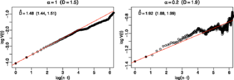
As an illustration, Figure 9 shows the log–log regression fit for the variation estimator of order $p=1$ and our example data. For instances of the use of the madogram estimator in the applied literature, see Weissel, Pratson and Malinverno (1994) and Zaiser et al. (2004).

Figure 9: Log–log regression for the madogram estimator [variation estimator (18) with power index $p=1$] and the datasets in the lower row of Figure 1. Only the two points marked with filled circles are used when fitting the regression line.

A natural question then is for the choice of the power index $p>0$. With the estimator depending on the relationship (4) between the fractal index, $\alpha$, in the expansion (15) and the Hausdorff dimension, $D$, of the sample path, it is critically important to assess its validity when the assumption of Gaussianity is violated. In the standard case in which $p=2$, Hall and Roy (1994) showed that, while the relationship (4) extends to some non-Gaussian processes, it fails easily. For example, it applies to marginally power-transformed Gaussian fields if and only if the transformation power exceeds $1/2$. Other counterexamples can be found in the work of Bruno and Raspa (1989) and Scheuerer (2010).

Bruno and Raspa (1989) and Bez and Bertrand (2011) applied the Lipschitz–Hölder heuristics ofMandelbrot [(1977), page 304] to argue that the relationship (4) is universal when $p=1$. While we agree that the relationship is particularly robust and inclusive when $p=1$, the Lipschitz–Hölder heuristics, which connects the Lipschitz exponent of a sample path to its Hausdorff dimension, is tied to continuity. Thus, it can fail if the sample paths are sufficiently irregular. For instance, the sample paths of a binary stochastic process, which attains the values 0 and 1 only, have Hausdorff dimension $D=1$. As the corresponding variogram (14) is independent of its order, we may refer to the common version as $\gamma$. If the expected number of sample path jumps per unit time is finite, then $\gamma$ grows linearly at the coordinate origin (Masry, 1972). In this case, the relationship (4) holds if, and only if, the common variogram, $\gamma$, is understood to be of order $p=1$. However, there are binary processes whose variogram behaves like $\gamma(t)=\mathcal{O}(|t|^{\gamma})$ as $t\to 0$, where $0<\gamma<1$, and then the relationship fails. Notwithstanding these examples, the argument of Bruno and Raspa (1989) and Bez and Bertrand (2011) is persuasive, and we maintain that the relationship (4) is particularly inclusive when $p=1$. A natural conjecture is that if $p=1$, then the relationship is valid if the process is ergodic (in a suitable sense) and the expected number of sample path discontinuities per unit time is finite. Furthermore, it is worth noting that there are processes for which the madogram exists and the foregoing is satisfied, while second moments do not exist (Ehm, 1981).

The following interesting connection between the Hall–Wood estimator and the madogram estimator also suggests a special role of the power index $p=1$. For $l$ a positive integer and $j=0,1,\ldots,l-1$, let

$$\widehat{A}^{(j)}(l/n)=\frac{l}{n}\sum_{i=1}^{\lfloor(n-j)/l\rfloor}\bigl{|}X_{(il+j)/n}-X_{(il+j-l)/n}\bigr{|}.$$

Then $\widehat{A}(l/n)=\widehat{A}^{(0)}(l/n)$ and

$$\widehat{V}_{1}(l/n)=\frac{1}{2}\frac{n}{n-1}\frac{1}{l}\sum_{j=0}^{l-1}\widehat{A}^{(j)}(l/n)$$

is, up to inessential constants, the mean of $l$ distinct copies of $\widehat{A}(l/n)$. A comparison of the general forms (9) and (2.4), or the standard forms (10) and (18), of the Hall–Wood estimator with the madogram estimator suggests that the latter is a statistically more efficient version of the Hall–Wood estimator. A similar, more tedious calculation can be used to argue heuristically that the box-count estimator has a bias, typically leading to lower estimates of the fractal dimension than the Hall–Wood and variation estimators. For a confirmation in simulation studies, see Section 3.2.

Figure 10: Root mean squared error (RMSE) of the variation estimator (18) as a function of the power exponent, $p$, for Gaussian fractional Brownian motion (left) and Gaussian processes with powered exponential covariance (right). The scale parameter used is $c=1$, and each RMSE is computed from 1,000 Monte Carlo replicates of Gaussian sample paths under the sampling scheme (6), where $n=1{,}024$. The curves correspond to fixed values of the fractal index, $\alpha$, and have their minima marked.

Figure 11: Same as Figure 10, except that in each sample path a randomly placed observation is contaminated by an additive Gaussian outlier with standard deviation $0.1$.

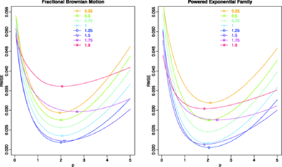
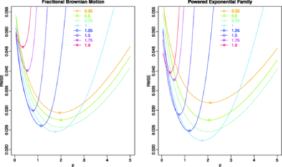
Here we restrict attention to a small initial study that assesses the efficiency and outlier resistance of variation estimators. Figures 10 and 11 show the root mean squared error (RMSE) of the variation estimator (18) from Gaussian sample paths in dependence on the power index, $p$. The curves are computed from 1,000 independent realizations with sample size $n=1{,}024$, correspond to fixed values of the fractal index, $\alpha$, and have their minima marked. Figure 10 concerns the ideal Gaussian model, where the estimator performs best for power indices of about $p=2$, corresponding to the variogram estimator, similarly to the observations of Coeurjolly [(2001), page 1417]. Figure 11 shows that the RMSE can deteriorate considerably under a single additive outlier, with the effect being stronger for smoother sample paths, that is, higher values of the fractal index. The smaller the power index, the more outlier resistant the variation estimator.

A possible variant of the variation estimator uses $p$-moments of higher increments, as proposed by Kent and Wood (1997) and Istas and Lang (1997) in the case $p=2$. For example, one could turn to second differences, rather than first differences, and base a log–log regression on

$$\quad\widehat{V}_{p}^{(2)}(l/n) = \frac{1}{2(n-2l)}$$

$${}\cdot\sum_{i=l}^{n-l}\bigl{|}X_{(i+l)/n}-2X_{i/n}+X_{(i-l)/n}\bigr{|}^{p},$$

rather than the standard variation (16). Also, if more than two points are used in the regression, the generalized least squares method could be used in lieu of the ordinary least squares technique. However, there is no clear advantage in doing so in applied settings, in which the corresponding covariance structure is unknown and needs to be estimated as well.

2.5 Spectral and Wavelet Estimators

We now consider the semi-periodogram estimator of Chan, Hall and Poskitt (1995), which operates in the frequency domain and is closely related to the spectral estimator of Dubuc et al. (1989a). The basis for this estimator is the well-known fact that the spectral density function for a stationary stochastic process with a second-order variogram of the form (3) decays like $|\omega|^{-\alpha-1}$ as frequency $|\omega|\to\infty$ (Stein, 1999). For a stationary Gaussian process $\{X_{t}\dvtx t\in[0,1]\}$, Chan, Hall and Poskitt (1995) defined

$$B(\omega)=2\int_{0}^{1}X_{t}\cos(\omega[2t-1])\,{\rm d}t$$

and called

$$J(\omega)=B(\omega)^{2}$$

the semi-periodogram. Under weak regularity conditions, the expected value of the semi-periodogram decays in the same way as the spectral density function. Suppose now that we have $n_{s}=2m+1$ observations $X_{t}$ at times $t=i/(2m)$, where $i=0,1,\ldots,2m.$ In this setting, Chan, Hall and Poskitt (1995) approximated $B(\omega)$ by

$$\widehat{B}(\omega)=\frac{1}{m}\Biggl{[}\frac{X_{0}+X_{1}}{2}+\sum_{i=1}^{2m-1}X_{i/(2m)}\cos\biggl{(}\omega\frac{i-m}{m}\biggr{)}\Biggr{]}$$

and the semi-periodogram $J(\omega)$ by

$$\widehat{J}(\omega)=\widehat{B}(\omega)^{2}.$$

The semi-periodogram estimator of the fractal dimension $D$ is

$$\widehat{D}_{{\mathrm{P}}} = \frac{5}{2}+\frac{1}{2}\Biggl{\{}\sum_{l=1}^{L}(s_{l}-\bar{s})\log\widehat{J}(\omega_{l})\Biggr{\}}$$

$${}\hskip 16.0pt\cdot\Biggl{\{}\sum_{l=1}^{L}(s_{l}-\bar{s})^{2}\Biggr{\}}^{-1},$$

where $\omega_{l}=2\pi l$, $s_{l}=\log\omega_{l}$ and $\bar{s}$ is the mean of $s_{1},\allowbreak\ldots,s_{L}$. The highest unaliased frequency (i.e., the Nyquist frequency) is $\pi m$, which is reflected by the fact that $\widehat{B}(\pi m+\delta)=\widehat{B}(\pi m-\delta)$ for any $\delta$. This suggests setting $L=\lfloor m/2\rfloor$, but Chan, Hall and Poskitt (1995) recommended using $L=\lfloor\min\{m/2,n_{s}^{2/3}\}\rfloor$, which is less than $\lfloor m/2\rfloor$ for $m\geq 34$. As $m$ grows, this rule thus has the effect of eliminating $\widehat{J}(\omega)$ at high frequencies in forming $\widehat{D}_{{\mathrm{P}}}$, which at first seems counterintuitive, given that the underlying scaling law applies as $\omega$ increases. However, as $\omega$ approaches the Nyquist frequency, aliasing causes the expectation of $\widehat{J}(\omega)$ to deviate markedly from the decay rate of $\omega^{-\alpha-1}$, leading to the need to eliminate high-frequency terms when forming $\widehat{D}_{{\mathrm{P}}}$. Figure 12 shows an example of the log–log regression for the semi-periodogram estimator for datasets from Figure 1, where $n_{s}=1{,}025$ and hence $L=101<m/2=256$.

Figure 12: Log-log regression for the semi-periodogram estimator and the datasets in the lower row of Figure 1. Only the points marked with filled circles are used when fitting the regression line.

Figure 13: Log–log regression for the DCT-II estimator and the datasets in the lower row of Figure 1. Only the points marked with filled circles are used when fitting the regression line.

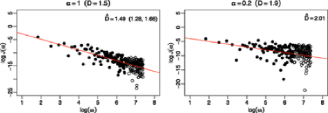
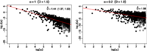
The definition of $\widehat{B}(\omega)$ is similar in spirit to the so-called type-II discrete cosine transform (DCT-II); see Ahmed, Natarajan and Rao (1974) and Strang (1999) for background. Davies (2001) noted that this transform has some attractive properties when used as a basis for spectral analysis, so it is of interest to explore the DCT-II as a substitute for the semi-periodogram in estimating fractal dimension. Given time series data of the form (6), taking the definition of the DCT-II given by Gonzalez and Woods (2007) and adjusting it for our convention for the samples $X_{i/(2m)}$ yields

$$\widetilde{B}(\omega)=\biggl{(}\frac{2}{2m+1}\biggr{)}^{1/2}\sum_{i=0}^{2m}X_{i/(2m)}\cos\biggl{(}\omega\frac{2i+1}{4m}\biggr{)}$$

and $\widetilde{J}(\omega)=\widetilde{B}(\omega)^{2}$. Here the Nyquist frequency is $2\pi m$, as can be seen by noting that $\widetilde{J}(2\pi m+\delta)=\widetilde{J}(2\pi m-\delta)$ for any $\delta$. If we now let $\omega_{l}=2\pi lm/(2m+1)$ with $s_{l}=\log\omega_{l}$ and $\bar{s}$ being the mean of the $s_{l}$’s as before, the log–log regression estimator (2.5) can be applied with $\widehat{J}(\omega_{l})$ replaced by $\widetilde{J}(\omega_{l})$ and $L=\lfloor\min\{2m,4n_{s}^{2/3}\}\rfloor$. The DCT-II estimator uses approximately four times more points in the log–log regression than does the semi-periodogram estimator. For example, in Figure 13 we have $L=406$, whereas we had $L=101$ in Figure 12.

Figure 14: Log–log regression for the wavelet estimator and the datasets in the lower row of Figure 1. Only the points marked with filled circles are used when fitting the regression line.

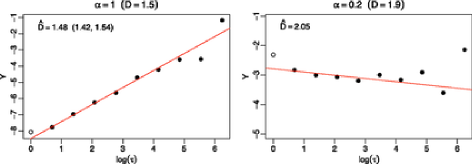
The semi-periodogram estimator also serves as motivation for a similar wavelet estimator, which is an adaptation of a weighted least squares estimator for the long memory parameter of a fractionally differenced process (Percival and Walden, 2000, Section 9.5). Given a time series of length $n_{s}$, we compute its maximal overlap discrete wavelet transform (MODWT) out to level $J_{0}=\lfloor\log_{2}(n_{s})\rfloor$ using reflection boundary conditions; this can be done using the function modwt in the R package wavelets (Aldrich, 2010). This MODWT yields $J_{0}$ vectors of wavelet coefficients $\widetilde{\bf W}_{j}$, $j=1,\ldots,J_{0}$, each of which contains $2n_{s}$ coefficients. The coefficients in the $j$th vector are associated with the scale $\tau_{j}=2^{j-1}$. The average of these coefficients squared, that is, $\|\widetilde{\bf W}_{j}\|^{2}/2n_{s}$, provides an estimator of the wavelet variance $\nu^{2}(\tau_{j})$. This variance varies approximately as $\tau_{j}^{\alpha}$ for large $\tau_{j}$ [Percival and Walden, 2000, equation (297b)],where $\alpha$ is the fractal index, from which the fractal dimension can be deduced; see Table 2. The scale $\tau_{j}$ corresponds to the band of frequencies $(\pi/2^{j},\pi/2^{j-1}]$.

The information that is captured by the semi-periodogram at high frequencies is thus captured in the wavelet variance at small scales $\tau_{j}$. Since Chan, Hall and Poskitt (1995) eliminated certain high frequencies in their semi-periodogram estimator, this suggests using just the wavelet variances indexed by $j=J_{0},\ldots,J_{1}$, where $J_{0}=\max\{1,\lfloor\log_{2}(n_{s})/3-1\rfloor\}$. Because the variance of the wavelet variance estimators depends upon $\tau_{j}$, we replace the ordinary least squares estimator of the slope that is the basis for equation (2.5) with a weighted least squares estimator, say $\hat{\alpha}_{\rm WL}$ [Percival and Walden, 2000, equation (376c)]. The corresponding estimator of the fractal dimension $D$ is $\widehat{D}_{\rm WL}=2-\frac{1}{2}\hat{\alpha}_{\rm WL}$. Figure 14 gives an example of the wavelet estimator of $D$. Note that the estimator of $D$ in the right-hand plot is $\widehat{D}_{\rm WL}=2.05$, which is greater than the upper limit $D=2$ for the Hausdorff dimension of a curve. Sampling variability can cause this to happen on occasion with the other estimators also. In the simulation experiments reported below, the wavelet estimator proved to perform comparably to the DCT-II estimator, so we have chosen to drop the former and report only on the latter in what follows.

3 Performance Assessment: Time Series and Line Transect Data

We now turn to an evaluation of the various types of estimators, where we consider the large sample behavior under infill asymptotics and report on a finite sample simulation study that assesses both efficiency and robustness.

3.1 Asymptotic Theory

As noted, the fractal dimension refers to the properties of a graph in a hypothetical limiting process that might exist if the scale of measurement were to become infinitely fine. Hence, estimators of fractal dimension are studied under infill asymptotics (Hall and Wood, 1993; Stein, 1999), in which the number of observations grows to infinity, whereas the underlying domain, namely the unit interval, remains fixed. We assume that time series or line transect data of the form (6) arise from a Gaussian process $\{X_{t}\dvtx t\in[0,1]\}$ with a second-order structure of the type (3), where we let $n$ grow without bounds. Typically, the literature assumes stationarity, so that the process $\{X_{t}\dvtx t\in[0,1]\}$ has a covariance function of the form

$$\sigma(t)=\sigma(0)-|ct|^{\alpha}+\mathcal{O}(|t|^{\alpha+\beta})\quad\mbox{as }t\to 0,$$

where $\alpha\in(0,2)$, $\beta\geq 0$ and $c>0$. The behavior of the bias, variance and mean squared error (MSE) of the estimators, and the corresponding types of limit distributions, then depend on the fractal index $\alpha$ and on $\beta$. Typically, the corresponding asymptotic results carry over to Gaussian processes with stationary increments and a variogram or structure function of the form (3).

For any Hall–Wood or variogram estimator $\widehat{D}$ of the form (9) or (2.3) with a fixed value of the design parameter $L$, the key results of Hall and Wood (1993) and Constantine and Hall (1994) are that

$$\mbox{MSE}(\widehat{D})$$

$$\quad=\cases{\mathcal{O}(n^{-1})+\mathcal{O}(n^{-2\beta}),&\mbox{if }$0<\alpha<\frac{3}{2}$,\cr\mathcal{O}(n^{-1}\log n)+\mathcal{O}(n^{-2\beta}),&\mbox{if }$\alpha=\frac{3}{2}$,\cr\mathcal{O}(n^{2\alpha-4})+\mathcal{O}(n^{-2\beta}),&\mbox{if }$\frac{3}{2}<\alpha<2$,}$$

where in each case the first term corresponds to the variance, and the second term to the squared bias. If $\alpha\leq 3/2$, then $\widehat{D}$ has a normal limit; if $\alpha>3/2$, the limit is a Rosenblatt distribution as described by Taqqu (1975). In a recent far-reaching paper, Coeurjolly (2008) showed that in the Gaussian case and for the variation estimator (2.4) with general power index $p>0$, the asymptotic behavior is still described by (3.1). Furthermore, the convergence rates are retained if the arithmetic mean in the definition of the power variation (16) is replaced by a trimmed mean, or by a convex combination of sample quantiles. While some of these results carry over to certain specific non-Gaussian processes (Chan and Wood, 2004; Achard and Coeurjolly, 2010), the limiting distribution theory is considerably richer then, and a general non-Gaussian theory remains lacking.

Figure 15: Root mean squared error (RMSE) of estimators of fractal dimension in dependence on the sample size, $n$, computed from Gaussian sample paths of the form (6) with powered exponential covariance function, $\sigma(t)=\exp(-|t|^{\alpha})$. For each combination of $\alpha$ and $n$, the number of Monte Carlo replicates is 1,000.

It is interesting to observe the change in the asymptotic rate of convergence at $\alpha=3/2$ for all these types of estimators. However, Kent and Wood (1997) showed that the variogram estimator achieves an MSE of order

$$\mbox{MSE}(\widehat{D})=\mathcal{O}(n^{-1})+\mathcal{O}(n^{-2\beta})$$ (22)

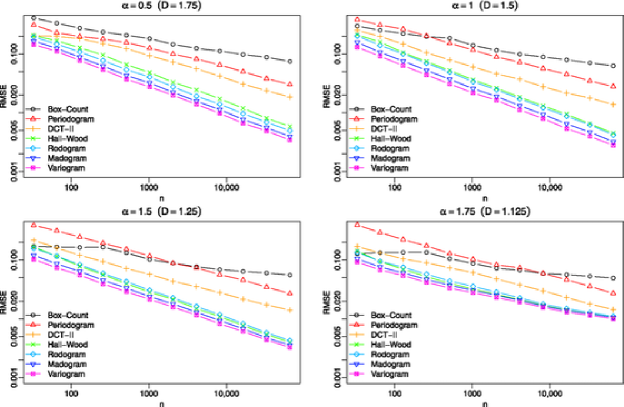
for all $\alpha\in(0,2)$ if the design parameter satisfies $L\geq 3$ and the generalized least squares technique, rather than the ordinary least squares method, is used in the log–log regression fit, and/or second differences of the form (2.4) are used. Similarly, Coeurjolly (2008) demonstrated that the asymptotic rate of convergence for the variation estimator with general power index $p>0$ can be improved if second differences or related special types of increments are used. In finite sample simulation studies for the variogram estimator ($p=2$), Kent and Wood (1997) did not find a clear-cut advantage in using generalized least squares and/or second differences, and our own experience with variation estimators of diverse power indices is similar. As Kent and Wood (1997) argued, the likely cause is that, the closer $\alpha$ is to 2, the larger $n$ must be before the asymptotic regime is reached. This behavior is in marked contrast to the case of spatial lattice data, to be discussed below.

Chan, Hall and Poskitt (1995) developed asymptotic theory for the semi-periodogram estimator, but the MSE decays at best at rate $\mathcal{O}(n^{-1/4})$ in their results. The asymptotic scenario for the level crossing estimator in Feuerverger, Hall and Wood (1994) involves a bandwidth parameter and thus is not directly comparable.

3.2 Simulation Study: Gaussian Processes

We now turn to a simulation study, in which we confirm and complement the foregoing asymptotic results in a Gaussian setting. In doing so, exact simulation is critically important (Chan and Wood, 2000; Zhu and Stein (2002)), and we use the circulant embedding approach (Dietrich and Newsam 1993; Wood and Chan, 1994; Stein, 2002; Gneiting et al., 2006) as implemented in the R package RandomFields (Schlather, 2001) to generate Gaussian sample paths, using the function GaussRF. The circulant embedding technique relies on the fast Fourier transform and is both exact and fast.

Figure 16: Boxplots for estimates of the fractal dimension from Gaussian sample paths of the form (6), where $n=1{,}024$, with powered exponential covariance function, $\sigma(t)=\exp(-|t|^{\alpha})$, and the fractal index, $\alpha$, being equal to 0.4, 1.0 and 1.6, respectively. The corresponding true values of the fractal dimension, $D$, namely 1.8, 1.5 and 1.2, are shown as dashed lines. The number of Monte Carlo replicates is 500.

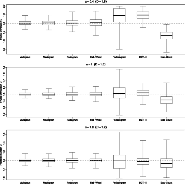
Figure 15 shows log–log plots for the root mean squared error (RMSE) of the various types of estimators in their dependence on the sample size $n$, computed from 1,000 independent trajectories of the form (6) from the corresponding stationary Gaussian process with a powered exponential covariance function, $\sigma(t)=\exp(-|t|^{\alpha})$. The graphs are approximately linear, and their slopes show good agreement with the asymptotic laws in (3.1). Furthermore, they confirm the aforementioned observation of Kent and Wood (1997) that large values of the fractal index, $\alpha$, require large sample sizes to reach the asymptotic regime. The variogram estimator generally shows the lowest MSE, followed by the madogram and rodogram, and then the Hall–Wood, DCT-II, periodogram and box-count estimators. This ranking is retained under Gaussian processes with covariance functions from the Matérn and Cauchy families, as well as for fractional Brownian motion, for all values of the fractal index $\alpha$ and all sufficiently large sample sizes, $n$. The use of variation estimators based on second differences, as defined in (2.4), typically does not yield lower RMSEs (results not shown).

Figure 17: Scatterplot matrix for estimates of the fractal dimension from Gaussian sample paths of the form (6) with exponential covariance function, $\sigma(t)=\exp(-|t|)$, and sample size $n=1{,}024$. The true value of the fractal dimension is $D=1.5$. The panels along the diagonal show histograms of the estimates, and those above the diagonal pairwise Pearson correlation coefficients. The number of Monte Carlo replicates is 500.

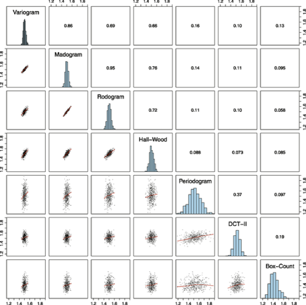
Figures 16 and 17 show box- and scatterplots for the same types of estimators and the same class of Gaussian processes, where the sample size is $n=1{,}024$. Three groups of estimators can be distinguished, the first comprising the variogram and other two variation estimators along with the Hall–Wood estimator, the second the spectral estimators, and the third the box-count estimator. The most efficient estimator is the variogram estimator, closely followed by the madogram estimator. As we have argued theoretically before, the madogram estimator is a more efficient version of the Hall–Wood estimator, in that the estimators are strongly correlated, but the former is less dispersed. While the spectral estimators are less competitive, showing substantially higher dispersion than the variation estimators, the DCT-II estimator improves considerably on the periodogram estimator. The box-count estimator generally shows a bias, with the estimates being too low.

Figure 18: Estimates of the fractal dimension plotted at the midpoints of a sliding estimation window of size $1{,}025$, for a Gaussian sample path of the form (6), where $n=10{,}000$, with exponential covariance function, $\sigma(t)=\exp(-|t|)$. The true fractal dimension, $D=1.5$, is marked by the dashed line. The label on the horizontal axis, $i$, indicates the midpoint of the sliding estimation block, at $i/10{,}000$.

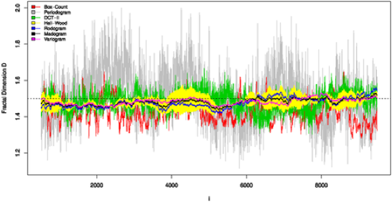
Figure 18 illustrates these results in a further experiment, in which we consider a Gaussian sample path with the exponential covariance function, $\sigma(t)=\exp(-|t|)$, and estimate the fractal dimension along sliding blocks of size $1{,}024$. The corresponding estimates are plotted at the midpoint of the sliding block. It is clearly seen that the variogram and other variation estimators are the least dispersed, and that the madogram estimator is a more efficient version of the Hall–Wood estimator. The spectral estimators are the most dispersed, with the DCT-II estimator outperforming the periodogram estimator, and the box-count estimator is biased.

Thus far in this section, we have studied the efficiency of the estimators under an ideal Gaussian process assumption. However, robustness against deviations from Gaussianity is a critically important requirement on any practically useful estimator of the fractal dimension. In this light, we now expand our simulation study, and consider a situation in which Gaussian sample paths are contaminated by additive outliers. Specifically, given a sample path of the form (6), we let $i$ be discrete uniform on $\{0,1,\ldots,n\}$ and replace $X_{i/n}$ by $X_{i/n}+y$, where $y$ is normal with mean zero and standard deviation 0.1 and independent of $i$. This process is repeated to obtain the desired number of outliers.

Figure 19: Root mean squared error (RMSE) of estimators of fractal dimension in dependence on the fractal index, $\alpha$, for Gaussian sample paths of the form (6) with sample size $n=1{,}024$ and powered exponential covariance function, $\sigma(t)=\exp(-|t|^{\alpha})$. The panel on the left corresponds to the ideal Gaussian process setting; the panel on the right to a situation with five additive outliers in each sample path. The number of Monte Carlo replicates is 1,000.

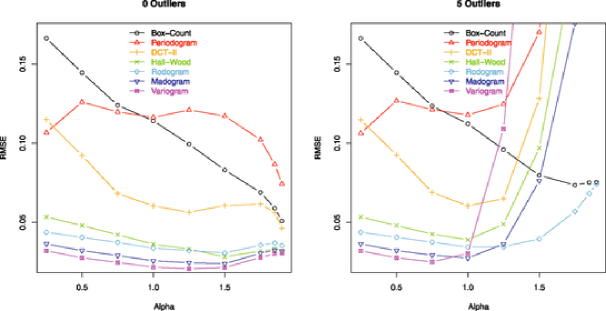
Figure 19 shows RMSEs from such an experiment, using sample size $n=1{,}024$, five additive outliers, and the powered exponential covariance function, $\sigma(t)=\exp(-|t|^{\alpha})$, with values of the fractal index $\alpha$ that nearly span the full range from 0 to 2. Not surprisingly, the results resemble those in Figures 10 and 11, which considered variation estimators and the case of a single outlier only, and echo the findings of Achard and Coeurjolly (2010). Amongst the variation estimators considered here, the most outlier resistant is the rodogram estimator ($p=1/2$), but the box-count estimator, which performs poorly overall when there are no outliers, becomes competitive at the highest $\alpha$ considered ($1.9$).

3.3 Discussion

The foregoing results and arguments lead us to a recommendation for practitioners, in that we join Bruno and Raspa (1989) and Bez and Bertrand (2011) and call for the use of the madogram estimator, that is, the variation estimator with power index $p=1$. The madogram estimator can be interpreted as a statistically superior version of the Hall–Wood estimator, is simultaneously more outlier resistant and more efficient than many of its competitors, and has strong intuitive appeal. Importantly, the critical relationship (4) between the fractal index of a stochastic process whose variogram of order $p$ shows a behavior of the form (1) at the origin, and the fractal dimension of its sample paths, is apparently valid for a larger class of non-Gaussian processes when $p=1$ than for certain other choices of $p$ (in particular, $p=2$), thereby justifying the use of the madogram estimator for both Gaussian and non-Gaussian stochastic processes. Its resistance to outliers can be enhanced further if the arithmetic mean in the definition of the power variation (16) is replaced by a trimmed mean, as proposed by Coeurjolly (2008).

4 Estimating the Fractal Dimension of Spatial Data

We now turn to estimators of the fractal dimension of spatial data, as discussed by Dubuc et al. (1989b), Constantine and Hall (1994), Davies and Hall (1999), Chan and Wood (2000) and Zhu and Stein (2002), among other authors. Burrough (1981) noted a wealth of applications to landscape and other environmental data, with those of Rothrock andThorndike (1980) on the underside of sea ice, and Goff and Jordan (1988) on the topography of the sea floor, being particularly interesting examples.

From a probabilistic point of view, a natural initial question is for the theoretical relationship between the fractal dimension of a surface indexed in $\mathbb{R}^{2}$, and the fractal dimension of its sections or line transects. Assuming stationarity of the spatial random field and additional (weak) regularity conditions, Hall and Davies (1995) showed that the fractal dimensions along line transects are all identical to one another, except that in one special direction the dimension may be less than in all others. Very general results that do not depend on the stochastic process setting are available from the fundamental work of Marstrand (1954). We join Davies and Hall (1999) in arguing that these results provide substantial support for the use of fractal dimension as a canonical measure of surface roughness. In particular, they allow us to estimate the fractal dimension of a surface by adding 1 to any estimate of the fractal dimension of the corresponding line transects.

Technically, we focus discussion on the situation in which a spatial stochastic process, indexed by the unit square in $\mathbb{R}^{2}$, is sampled on a regular lattice, to yield a surface graph of the form

$$\left\{(t,X_{t})\dvtx t=\pmatrix{t_{1}\cr t_{2}}=\frac{1}{n}\pmatrix{i_{1}\cr i_{2}},i_{1}=0,1,\ldots,n,\right.$$

$${}\hskip 39.0pt\left.\vphantom{\pmatrix{t_{1}\cr t_{2}}}i_{2}=0,1,\ldots,n\right\}\subset\mathbb{R}^{3}.$$

Before reviewing estimators of fractal dimension studied in the extant literature, and introducing new estimators, we propose a simple, unified notation. Specifically, for $k>0$ we let

$$S(k) = \left\{(i_{1},i_{2},j_{1},j_{2})\in\{0,1,\ldots,n\}^{4}\dvtx\right.\vphantom{\pmatrix{i_{1}\cr i_{2}}}$$

$$\hskip 44.0pt{}\left.\hskip 3.0pt\left|\pmatrix{i_{1}\cr i_{2}}-\pmatrix{j_{1}\cr j_{2}}\right|=k\right\},$$

and denote the cardinality of this set by $N(k)$. If $N(k)>1$, we refer to $k$ as a relevant distance. The estimators in the subsequent Sections 4.1 to 4.2 then take the form

$$\widehat{D} = 2-\frac{1}{p}\biggl{\{}\sum_{k\in\mathcal{K}}(s_{k}-\bar{s})\log\widehat{V}_{p}(k/n)\biggr{\}}$$

$$\hskip 17.0pt{}\cdot\biggl{\{}\sum_{k\in\mathcal{K}}(s_{k}-\bar{s})^{2}\biggr{\}}^{-1},$$

where $\mathcal{K}$ is a finite collection of relevant distances, $s_{k}=\log(k/n)$, $\bar{s}$ is the mean of $\{s_{k}\dvtx k\in\mathcal{K}\}$, and $\widehat{V}_{p}(k/n)$ is a certain variation with general power index $p>0$.

Two-dimensional geometry allows for many options in the choice of the distance representatives and the variation, and we restrict attention to the most plausible and best performing estimators in the literature, all of which are based on power variations (Davies and Hall, 1999; Chan and Wood, 2000; Zhu and Stein (2002)). As concerns the set $\mathcal{K}$ of distance representatives, simulation experiments, experience in the line transect case, and the work of Chan and Wood (2000) and Zhu and Stein (2002) all suggest that a restriction to the smallest relevant distances only tends to lead to the best performance. In addition to minimizing the bias of the estimator, this strategy keeps the computational complexity low as well.

4.1 Isotropic Estimator

Davies and Hall (1999) considered an estimator based on the isotropic empirical variogram, which we now generalize. For a relevant distance $k$, consider the variation

$$\quad\widehat{V}_{{\rm ISO};p}(k/n) = \frac{1}{2N(k)}$$

$${}\cdot\sum_{S(k)}|X_{i_{1}/n,i_{2}/n}-X_{j_{1}/n,j_{2}/n}|^{p}$$

with general power index $p>0$. The isotropic estimator $\widehat{D}_{{\rm ISO};p}$ with power index $p$ then is defined by (4) with the set $\mathcal{K}=\{1,\sqrt{2},2\}$ of distance representatives and the variation $\widehat{V}$ given by (4.1). Thus, we consider variations at horizontal and verticalspacings of one and two grid points ($k=1$ and $k=2$), and a diagonal spacing of a single grid point ($k=\sqrt{2}$), respectively.

4.2 Filter Estimator

Zhu and Stein (2002) studied a broad range of increment-based estimators, among which the “Filter 1” estimator shows good performance. We generalize by defining a filter estimator with general power index $p>0$, rather than just $p=2$ as in the work of Zhu and Stein (2002). Specifically, for a relevant distance $k>0$ let

$$\widehat{V}_{{\rm F};p}(k/n) = \frac{1}{2N(k)}$$

$${}\cdot\sum_{S(k)}\bigl{|}X_{i_{1}/n,i_{2}/n}$$

$${}\hskip 25.0pt-2X_{(i_{1}+j_{1})/(2n),(i_{2}+j_{2})/(2n)}$$

$${}\hskip 63.0pt\hskip 25.0pt+X_{j_{1}/n,j_{2}/n}\bigr{|}^{p}.$$

The filter estimator $\widehat{D}_{{\rm F};\hskip 0.85358ptp}$ with power index $p$ then is defined by (4) with the set $\mathcal{K}=\{2,2\sqrt{2},4\}$ of distance representatives and the variation $\widehat{V}$ given by (4.2). This considers variations at horizontal and vertical spacings of one and two grid points ($k=1$ and $k=2$), and a diagonal spacing of a single grid point ($k=\sqrt{2}$), respectively. Hence, the filter estimator is the natural equivalent of the isotropic estimator $\widehat{D}_{{\rm ISO};p}$, but now using second differences, rather than first differences.

4.3 Square Increment Estimator

The square increment estimator is based on a proposal of Chan and Wood (2000), who restrictedattention to quadratic variations. Here we definea square increment variation of general power index $p>0$, namely,

$$\widehat{V}_{{\rm SI};p}(k/n) = \frac{1}{2N(k)}$$

$${}\cdot\sum_{S(k)}|X_{i_{1}/n,i_{2}/n}-X_{i_{1}/n,j_{2}/n}$$

$${}\hskip 25.0pt-X_{j_{1}/n,i_{2}/n}+X_{j_{1}/n,j_{2}/n}|^{p},$$

where $k$ is a relevant distance. The square increment estimator $\widehat{D}_{{\rm SI};p}$ then is defined by (4) with the set $\mathcal{K}=\{\sqrt{2},2\sqrt{2}\}$ of distance representatives, corresponding to squares that have side widths of one and two grid points, and the variation $\widehat{V}$ given by (4.3).

4.4 Transect Estimators

Finally, we consider two very simple estimators that are based on the variation estimator $\widehat{D}_{{\mathrm{V}};p}$ with general power index $p>0$ of Section 2.4, or a variant that uses second differences, as defined in equation (2.4). In either case, a line transect estimate of the fractal dimension is computed for each row and each column in the grid. The transect-variation and transect-increment estimators $\widehat{D}_{{\rm TV};p}$ and $\widehat{D}_{{\rm TI};p}$ with power index $p$ then add 1 to the median of the $2n$ corresponding line transect estimates. In the former case, the line transect estimates are based on first differences, in the latter on second differences.

5 Performance Assessment: Spatial Data

We now assess the estimators by their large sample behavior under infill asymptotic as well as in finite sample simulation studies, considering both efficiency and robustness.

Figure 20: Root mean squared error (RMSE) for estimators of fractal dimension for data of the form (4) from spatial stochastic processes with powered exponential covariance, $\sigma(t)=\exp(-|t|^{\alpha})$, versus the (square root of the) sample size, $n$. The power index used is $p=2$, and for each combination of $\alpha$ and $n$, the number of Monte Carlo replicates is 1,000.

5.1 Asymptotic Theory

Davies and Hall (1999), Chan and Wood (2000) and Zhu and Stein (2002) developed asymptotic theory for a very wide range of estimators of the form (4) that are based on variations with power index $p=2$. Generally, their results apply under an infill asymptotic scenario for sample paths of the form (4) from an intrinsically stationary Gaussian spatial process with fractal index $\alpha\in(0,2)$ and a variogram that behaves like (3) at the origin. For estimators that are based on variations corresponding to a first difference, the generic result is that

$$\mbox{MSE}(\widehat{D})$$

(28)

$$\quad=\cases{\mathcal{O}(n^{-2})+\mathcal{O}(n^{-4\beta}),&\mbox{if }$0<\alpha<1$,\cr\mathcal{O}(n^{-2}L(n))+\mathcal{O}(n^{-4\beta}),&\mbox{if }$\alpha=1$,\cr\mathcal{O}(n^{2\alpha-4})+\mathcal{O}(n^{-4\beta}),&\mbox{if }$1<\alpha<2$,}$$

where $L$ is a function which is slowly varying at infinity. If $\alpha\leq 1$, then $\widehat{D}$ has a normal limit, while, if $\alpha>1$, the limit is related to a Rosenblatt distribution, with some of these results carrying over to certain specific non-Gaussian processes (Chan and Wood, 2004). However, if the variations correspond to a second difference, such as in the cases of the filter and square increment estimators, and/or the generalized least squares techniques, rather than the ordinary least squares method, is used, an improved asymptotic behavior, namely,

$$\mbox{MSE}(\widehat{D})=\mathcal{O}(n^{-2})+\mathcal{O}(n^{-4\beta})$$ (29)

for all $0<\alpha<2$, is achieved, with an associated limit distribution that is normal. For regularity conditions and further detail, we refer to the original work of Davies and Hall (1999), Chan and Wood (2000), Zhu and Stein (2002) and Chan and Wood (2004), which is impressive. While these authors restricted attention to quadratic variations with power index $p=2$ only, we conjecture, based on the work of Guyon and León (1989), Istas and Lang (1997) and Barndorff-Nielsen, Corcuera and Podolskij (2009) on the power variations of Gaussian processes, that analogous results continue to hold under a general power index $p>0$, similar to the line transect case studied by Coeurjolly (2008).

As the amount of data in the sampling scheme (4) is about $n^{2}$, the asymptotic rates of convergence in (5.1) and (29) conform with those in the time series or line transect case, except that the transition from the classical to slower rates of convergence occurs already at $\alpha=1$ (or $D=3/2$), rather than at $\alpha=3/2$ (or $D=7/4$). Hence, these results suggest that there may be a higher benefit to using increments that are based on second differences in the spatial case than in the time series or line transect case.

5.2 Simulation Study: Gaussian Spatial Processes

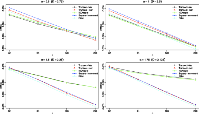
In the subsequent simulation study, we use state-of-the-art implementations of the circulant embedding method (Stein, 2002; Gneiting et al., 2006) to generate Gaussian sample surfaces. Figure 20 shows the root mean squared error (RMSE) of the estimators versus the (square root of the) sample size, $n$, using data of the form (4) from stationary spatial processes with powered exponential covariance function, $\sigma(t)=\exp(-|t|^{\alpha})$. The estimators use the traditional power index $p=2$, and the number of Monte Carlo replicates is 1,000.

The asymptotic rates of convergence in (5.1)and (29) suggest linear graphs with slope $-1$ on the logarithmic scale for the filter and square increment estimators and all values of the fractal index, $\alpha$. For the isotropic estimator, they suggest slope $-1$ for $\alpha\leq 1$, slope $-1/2$ for $\alpha=3/2$, and slope $-1/4$ for $\alpha=7/4$. Our empirical results are in good agreement with the theoretical slopes, and attest to the superior performance of the filter estimator in the ideal Gaussian process setting, as noted by Zhu and Stein (2002). Also, these and other simulation results lead us to conjecture that the transect-variation estimator behaves like (5.1), while the transect-increment estimator shares the favorable uniform asymptotic rate of convergence in (29).

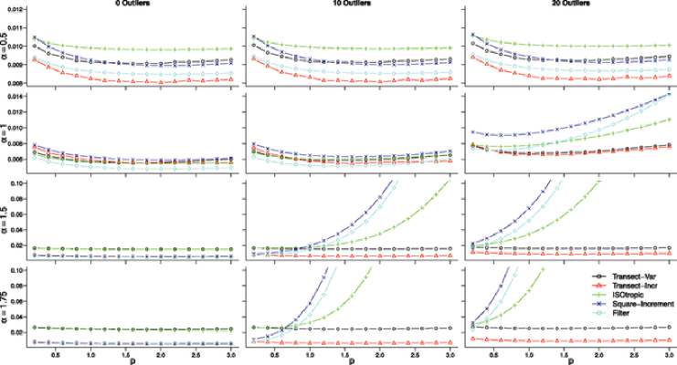
In Figure 21 we consider estimators with general power index $p>0$, but fix $n=256$ in the spatial sampling scheme (4). Again, we use the powered exponential covariance model, and the number of Monte Carlo replicates is 1,000, each comprising a total of $(n+1)^{2}=66{,}049$ observations within the unit square. The left column shows the RMSE in the ideal Gaussian process setting, in which the filter, square increment and transect-increment estimators perform best. Furthermore, the efficiency of these estimators depends only very little on the choice of the power index.

Figure 21 also studies the behavior of the estimators in the presence of outliers. Specifically, the middle and right-hand columns show RMSEs in situations in which the Gaussian sample paths have been contaminated by 10 and 20 additive outliers, respectively, in ways essentially identical to those described in Section 3.2. Note that the vertical scale differs from row to row, with the largest RMSEs corresponding to the smoothest surfaces. The smoother the surface, that is, the larger the value of the fractal index, $\alpha$, the more impact the outliers have on the estimators. Two of the estimators that dominate in the uncontaminated setting, namely the filter and the square increment estimators, are the least outlier resistant, even though the outlier fraction is very small in our study, at 0.015 and 0.03 percent, respectively. The most resistant estimators are the transect estimators.

These results allow for an interpretation in terms of breakdown points. While comprehensive formal definitions of breakdown points for dependent data have recently become available (Genton and Lucas, 2003), it suffices here to take a heuristic point of view, and define the breakdown point of an estimator as the minimal fraction of contaminated data that can ruin an estimator. Evidently, the isotropic, filter and square increment estimators have breakdown point zero. In contrast, the transect estimators have a positive breakdown point of about $1/(2\sqrt{m})$ under the spatial sampling scheme (4), where $m\,{=}\,n^{2}$ is the approximate amount of data. To see this, note that each outlier affects the individual estimate for at most two of the $2n$ transects, from which the median is formed. Thus, a transect estimator cannot be ruined, unless a fraction of at least $(n/2)/n^{2}$, or $1/(2\sqrt{m})$, of the data are contaminated.

5.3 Discussion

While confirming extant theoretical and simulation results for spatial data, which suggest the use of variations that are based on second differences, the results of this section lead us to two novel insights.

Figure 21: Root mean squared error of isotropic, filter, square increment, transect-variation and transect-increment estimators of fractal dimension in dependence on the power index, $p$. The underlying sample paths are of the form (4) with $n=256$ from Gaussian spatial processes with powered exponential covariance, $\sigma(t)=\exp(-|t|^{\alpha})$. The columns correspond to situations with no outliers (left), 10 additive outliers (middle) and 20 additive outliers (right), respectively. The rows are for distinct values of the fractal index, namely $\alpha=0.5,1.0,1.5$ and $1.75$. The number of Monte Carlo replicates is 1,000.

Figure 22: Arctic sea-ice profiles, with the panels showing files sc98drft.002, 003 and 005–008, respectively, and the labels being in meters. See the text for details.

Thus far, the statistical literature has restricted attention to variation-based estimators with power index $p=2$. A first observation is that the efficiency of these estimators depends little on the power index, $p>0$. Outlier resistance and robustness arguments then suggest the use of smaller power indices, with Section 2.4 supporting the choice of $p=1$.

A second and potentially very surprising insight is the superior performance of the transect-variation and transect-increment estimators. These estimators have positive breakdown points and outperform the traditional estimators even under minimal deviations from the ideal Gaussian process setting. Indeed, in practice, we would expect much larger deviations than in our simulation setting, in which the outliers had substantially lower variability than the process itself, and occurred at fractions of about 1 in 6,000 and 1 in 3,000 only. As the transect-increment estimator appears to share the favorable uniform rate of convergence (29) with the best performing extant estimators, this suggests the availability of an estimator, namely the transect-increment estimator with power index $p=1$, that is both robust and efficient. We believe that these are highly promising prospects that deserve further study.

If spatial data are observed at irregularly scattered locations, rather than a regular grid, the only available estimator is a suitably modified version of the isotropic estimator (4.1), with $S(k)$ now representing pairs of stations that are approximately a distance $k$ apart. In such cases, the use of the power index $p=1$ again seems prudent.

6 Data Example: Arctic Sea-Ice Profiles

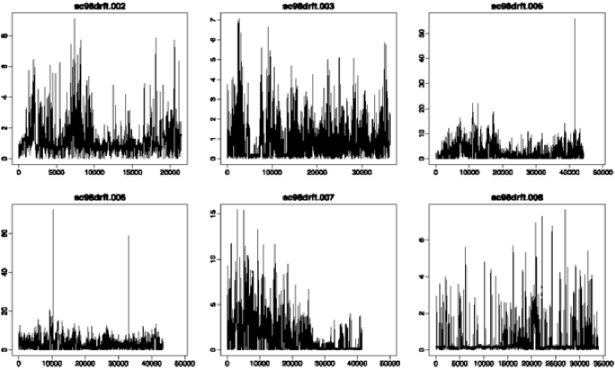
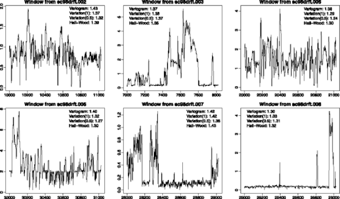
In this penultimate section, we estimate the fractal dimension of arctic sea-ice profiles based upon measurements of sea-ice draft (93% of thickness). These profiles can be regarded as line transectsthrough the underwater surface of sea ice because they were collected using upward-looking sonars by submarines traveling under the sea ice with no appreciable deviations from a single direction anddepth. The data used here were sampled one meter apart at a resolution of one meter by the U.S. Navy in August 1998 in the Arctic Ocean, and are available online from the National Snow and Ice Data Center at http://nsidc.org/data/docs/noaa/g01360_upward_looking_sonar. We examined six profiles of about 240 km total length (files sc98drft.002, 003 and 005–008). These profiles are illustrated in Figures 22 and 23 and show pronounced non-Gaussian features. Given the resolution, we join the extant literature in using fractal dimension to characterize the surface roughness of the macroscopic, topographic structure of sea ice, so that meters correspond to sufficiently small scales.

We use a sliding estimation window of width $n=1{,}024$ meters, move these blocks along the profiles in increments of 10 meters, and estimate fractal dimension for each of them, using variation estimators with power indices $p=2$ (variogram), $1$ (madogram) and $1/2$ (rodogram) along with the Hall–Wood estimator. Thus, for each method there are 23,303 blocks in total, with Figure 23 showing examples of profiles and dimension estimates. Figures 24 and 25 show the corresponding boxplots, histograms and pairwise scatter diagrams, composited over all blocks. While all four methods result in similar estimates, the strongest correlation is, not surprisingly, between the Hall–Wood and madogram estimators, with the latter being our estimator of choice.

Figure 23: Selected blocks of width 1,024 meters from the sea-ice profiles in Figure 22, along with the corresponding estimates of fractal dimension.

Figure 24: Boxplots for variation estimates with power indices $p=2$ (variogram), $1$ (madogram) and $1/2$ (rodogram) along with Hall–Wood estimates of fractal dimension for the blocks in the ice profile data. See the text for details.

Figure 25: Scatterplot matrix for variation estimates with power indices $p=2$ (variogram), $1$ (madogram) and $1/2$ (rodogram) along with Hall–Wood estimates of fractal dimension for the blocks in the ice profile data. See the text for details.

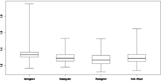
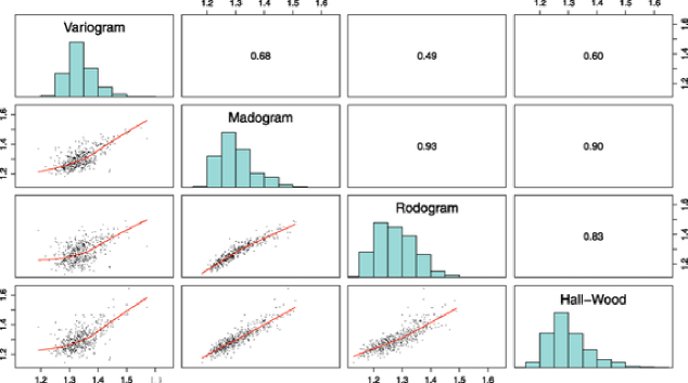
Overall, the Arctic sea-ice profiles have Hausdorff dimension of about 1.3 along line transects, and thus of about 2.3 spatially. These estimates are at the lower end of results reported in the literature. For instance, Bishop and Chellis (1989) argued that profiles of ice keels have fractal dimensions ranging from 1.2 to 1.7, while Connors, Levine and Shell (1990) reported estimates of about 1.4 and 1.6 for first year and multiyear ice segments, respectively. Further results and background information can be found in the works of Rothrock and Thorndike (1980) and Goff et al. (1995).

7 Concluding Remarks

In closing this review, we return to the opening quote of Lenny Smith [(2007), page 115] that precedes the abstract of our paper. Indeed, healthy skepticism about dimension estimates based on real-world data is well justified, in that estimates of fractal dimension depend on the availability of data at suitable scales and face issues of discreteness, and the effects of measurement error might also need to be disentangled. Notwithstanding these issues, estimates of fractal dimension can serve as informative descriptors of surface roughness.

In the case of time series or line transect data, we recommend the use of the madogram estimator, that is, the variation estimator with power index $p=1$. In the case of spatial lattice data, transect estimators based on madogram estimators along rows and columns show high promise. These recommendations echo observations of Bruno and Raspa (1989) and Bez and Bertrand (2011), who argued that the critical relationship (4) between the fractal index of a stochastic process whose variogram of order $p>0$ shows a behavior of the form (1) at the origin, and the fractal dimension of its sample paths, is particularly robust and inclusive when $p=1$. We encourage work toward rigorous results in these directions, including both variograms and their equivalents for general types of line transect and spatial increments.

Furthermore, we call for the development of large sample theory for variation estimators of general power index, including but not limited to our preferred choice of $p=1$. While for time series this has been achieved in the far-reaching recent work of Coeurjolly (2008), the case of spatial data remains open. As noted in Section 5.1, we believe that many of the results in the extant default case $p=2$ can be carried over to a general power index, $p>0$. In doing so, the results of Guyon and León (1989), Istas and Lang (1997) and Barndorff-Nielsen, Corcuera and Podolskij (2009) on the power variations of Gaussian processes provide tools that can be applied in concert with the methodology put forth in an impressive strand of asymptotic literature for $p=2$, which includes the work of Hall and Wood (1993), Constantine and Hall (1994), Kent and Wood (1997), Davies and Hall (1999), Chan and Wood (2000) and Zhu and Stein (2002), among others. Of particular interest is our conjecture in the spatial setting of Section 5.1, according to which the transect-variation approach allows for estimators of the fractal dimension that are simultaneously highly efficient and robust. This approach can be paired with the use of trimmed means or linear combinations of sample quantiles in defining power variations, as suggested by Coeurjolly (2008) for time series, or with the use of bipower and multipower variations (Barndorff-Nielsen et al. 2006; Barndorff-Nielsen, Corcuera and Podolskij, 2011). While the case of Gaussian processes appears to be challenging yet tractable, a general asymptotic theory for non-Gaussian processes remains elusive, despite the recent progress by Chan and Wood (2004) and Achard and Coeurjolly (2010).

To our knowledge, Bayesian methods for estimating fractal dimension have not been explored yet, except that the method of Handcock and Stein (1993) could be applied in a parametric context. Physical insight can drive the choice of the prior, and the development of Bayesian madogram estimators might be a promising option.

Multifractional Brownian motion (Peltier and Levy Vehel, 1995; Benassi, Jaffard and Roux, 1997; Herbin, 2006) is a generalization of the classical fractional Brownian motion, where the fractal dimension is allowed to vary along the sample paths. Similarly, the nonstationary Gaussian random fields described by Anderes and Stein (2011) allow for location-dependent, local Hausdorff dimensions, which need to be estimated as functions, rather than a single number. In this setting, the estimators considered in our paper can be used as building blocks for the more complex estimators needed to handle these nonstationary processes, as studied by Benassi, Cohen and Istas (1998), Ayache and Lévy Véhel (2004) and Coeurjolly (2005), among others. For an applied perspective, see Gagnon, Lovejoy and Schertzer (2006).

To close on a practical note, we have developed an R package, called fractaldim, that implements the estimators of fractal dimension discussed in this paper (Ševčíková, Gneiting and Percival, 2011). It has the ability to compute estimates for a single dataset, or a series of estimates along sliding blocks, as in our data example. Multiple estimates can be conveniently bundled into a single call, and the default arguments correspond to the recommendations in this paper.

For example, to generate four log–log plots of the type shown in Figure 5, a few lines of code suffice:

par(mfrow=c(2,2))
series <- GaussRF(x=c(0,1,1/1024),
  model=’stable’, gridtriple=TRUE,
  param=c(mean=0, variance=1,
  scale=1, kappa=1))
methods <- c(’hallwood’,
  ’periodogram’, ’variogram’,
  ’madogram’))
D <- fd.estimate(series,
  method=methods, plot.loglog=T,
  plot.allpoints=T)

Here, the function GaussRF from the RandomFields package is used to generate a Gaussian sample path with exponential covariance and fractal index $\alpha=1$. The desired estimation methods are passed to the estimation function, fd.estimate, as character strings as in our example. Alternatively, each method can be given as a list with a name element determining the method, and any additional elements specifying parameters. For example, an entry list(name=’variation’, p.index=1) is equivalent to ’madogram’.

To obtain interval estimates with a parametric bootstrap method, as proposed by Davies and Hall (1999) and shown in many of our figures, the following call suffices, using the simulated series from above, boot.it bootstrap replicates, and the madogram estimator:

D <- fd.estimate(series,
  methods=’madogram’)
D.boot <- rep(NA, boot.it)
alpha <- 4 - 2*D$fd
for (i in 1:boot.it)
 {
 boot.series <- GaussRF(
   x=c(0,1,1/1024), model=’stable’,
   gridtriple=TRUE,
   param=c(mean=0, variance=1,
   scale=D$scale^(-1/alpha),
   kappa=alpha))
 D.boot[i] <- fd.estimate(
   boot.series,
   methods=’madogram’)$fd
 }

Confidence intervals can be obtained from the array D.boot in the usual way. Additional functions for variation estimators in the line transect case are available within the dvfBm package (Coeurjolly,2009).

References

- Achard and Coeurjolly (2010) {barticle}[mr] \bauthor\bsnmAchard, \bfnmSophie\binitsS. and \bauthor\bsnmCoeurjolly, \bfnmJean-François\binitsJ.-F. (\byear2010). \btitleDiscrete variations of the fractional Brownian motion in the presence of outliers and an additive noise. \bjournalStat. Surv. \bvolume4 \bpages117–147. \biddoi=10.1214/09-SS059, issn=1935-7516, mr=2658892 \bptokimsref \endbibitem
- Adler (1981) {bbook}[mr] \bauthor\bsnmAdler, \bfnmRobert J.\binitsR. J. (\byear1981). \btitleThe Geometry of Random Fields. \bpublisherWiley, \baddressChichester. \bidmr=0611857 \bptokimsref \endbibitem
- Ahmed, Natarajan and Rao (1974) {barticle}[mr] \bauthor\bsnmAhmed, \bfnmN.\binitsN., \bauthor\bsnmNatarajan, \bfnmT.\binitsT. and \bauthor\bsnmRao, \bfnmK. R.\binitsK. R. (\byear1974). \btitleDiscrete cosine transform. \bjournalIEEE Trans. Computers \bvolumeC-23 \bpages90–93. \bidissn=0018-9340, mr=0356555 \bptokimsref \endbibitem
- Aldrich (2010) {bmisc}[auto:STB—2011/11/18—13:56:26] \bauthor\bsnmAldrich, \bfnmE.\binitsE. (\byear2010). \bhowpublishedWavelets: A package of funtions for computing wavelet filters, wavelet transforms and multiresolution analyses, R package version 0.2-6. \bptokimsref \endbibitem
- Anderes and Stein (2011) {barticle}[mr] \bauthor\bsnmAnderes, \bfnmEthan B.\binitsE. B. and \bauthor\bsnmStein, \bfnmMichael L.\binitsM. L. (\byear2011). \btitleLocal likelihood estimation for nonstationary random fields. \bjournalJ. Multivariate Anal. \bvolume102 \bpages506–520. \biddoi=10.1016/j.jmva.2010.10.010, issn=0047-259X, mr=2755012 \bptokimsref \endbibitem
- Ayache and Lévy Véhel (2004) {barticle}[mr] \bauthor\bsnmAyache, \bfnmAntoine\binitsA. and \bauthor\bsnmLévy Véhel, \bfnmJacques\binitsJ. (\byear2004). \btitleOn the identification of the pointwise Hölder exponent of the generalized multifractional Brownian motion. \bjournalStochastic Process. Appl. \bvolume111 \bpages119–156. \biddoi=10.1016/j.spa.2003.11.002, issn=0304-4149, mr=2049572 \bptokimsref \endbibitem
- Barndorff-Nielsen, Corcuera and Podolskij (2009) {barticle}[mr] \bauthor\bsnmBarndorff-Nielsen, \bfnmOle E.\binitsO. E., \bauthor\bsnmCorcuera, \bfnmJosé Manuel\binitsJ. M. and \bauthor\bsnmPodolskij, \bfnmMark\binitsM. (\byear2009). \btitlePower variation for Gaussian processes with stationary increments. \bjournalStochastic Process. Appl. \bvolume119 \bpages1845–1865. \biddoi=10.1016/j.spa.2008.09.004, issn=0304-4149, mr=2519347 \bptokimsref \endbibitem
- Barndorff-Nielsen Corcuera and Podolskij (2011) {bmisc}[auto:STB—2011/11/18—13:56:26] \bauthor\bsnmBarndorff-Nielsen, \bfnmO. E.\binitsO. E., \bauthor\bsnmCorcuera, \bfnmJ. M.\binitsJ. M. and \bauthor\bsnmPodolskij, \bfnmM.\binitsM. (\byear2011). \bhowpublishedMultipower variation for Brownian semistationary processes. Bernoulli 17 1159–1194. \bptokimsref \endbibitem
- Barndorff-Nielsen et al. (2006) {bincollection}[mr] \bauthor\bsnmBarndorff-Nielsen, \bfnmOle E.\binitsO. E., \bauthor\bsnmGraversen, \bfnmSvend Erik\binitsS. E., \bauthor\bsnmJacod, \bfnmJean\binitsJ., \bauthor\bsnmPodolskij, \bfnmMark\binitsM. and \bauthor\bsnmShephard, \bfnmNeil\binitsN. (\byear2006). \btitleA central limit theorem for realised power and bipower variations of continuous semimartingales. In \bbooktitleFrom Stochastic Calculus to Mathematical Finance \bpages33–68. \bpublisherSpringer, \baddressBerlin. \biddoi=10.1007/978-3-540-30788-4_3, mr=2233534 \bptokimsref \endbibitem
- Benassi, Cohen, and Istas (1998) {barticle}[mr] \bauthor\bsnmBenassi, \bfnmAlbert\binitsA., \bauthor\bsnmCohen, \bfnmSerge\binitsS. and \bauthor\bsnmIstas, \bfnmJacques\binitsJ. (\byear1998). \btitleIdentifying the multifractional function of a Gaussian process. \bjournalStatist. Probab. Lett. \bvolume39 \bpages337–345. \biddoi=10.1016/S0167-7152(98)00078-9, issn=0167-7152, mr=1646220 \bptokimsref \endbibitem
- Benassi, Jaffard, and Roux (1997) {barticle}[mr] \bauthor\bsnmBenassi, \bfnmAlbert\binitsA., \bauthor\bsnmJaffard, \bfnmStéphane\binitsS. and \bauthor\bsnmRoux, \bfnmDaniel\binitsD. (\byear1997). \btitleElliptic Gaussian random processes. \bjournalRev. Mat. Iberoam. \bvolume13 \bpages19–90. \bidissn=0213-2230, mr=1462329 \bptokimsref \endbibitem
- Berg, Mateu, and Porcu (2008) {barticle}[mr] \bauthor\bsnmBerg, \bfnmChristian\binitsC., \bauthor\bsnmMateu, \bfnmJorge\binitsJ. and \bauthor\bsnmPorcu, \bfnmEmilio\binitsE. (\byear2008). \btitleThe Dagum family of isotropic correlation functions. \bjournalBernoulli \bvolume14 \bpages1134–1149. \biddoi=10.3150/08-BEJ139, issn=1350-7265, mr=2543589 \bptokimsref \endbibitem
- Bez and Bertrand (2011) {bmisc}[auto:STB—2011/11/18—13:56:26] \bauthor\bsnmBez, \bfnmN.\binitsN. and \bauthor\bsnmBertrand, \bfnmS.\binitsS. (\byear2011). \bhowpublishedThe duality of fractals: Roughness and self-similarity. Theoretical Ecology 4 371–383. \bptokimsref \endbibitem
- Bishop and Chellis (1989) {bmisc}[auto:STB—2011/11/18—13:56:26] \bauthor\bsnmBishop, \bfnmG. C.\binitsG. C. and \bauthor\bsnmChellis, \bfnmS. E.\binitsS. E. (\byear1989). \bhowpublishedFractal dimension: A descriptor of ice keel surface roughness. Geophysical Research Letters 16 1007–1010. \bptokimsref \endbibitem
- Block, von Bloh, and Schellnhuber (1990) {barticle}[mr] \bauthor\bsnmBlock, \bfnmA.\binitsA., \bauthor\bparticlevon \bsnmBloh, \bfnmW.\binitsW. and \bauthor\bsnmSchellnhuber, \bfnmH. J.\binitsH. J. (\byear1990). \btitleEfficient box-counting determination of generalized fractal dimensions. \bjournalPhys. Rev. A (3) \bvolume42 \bpages1869–1874. \biddoi=10.1103/PhysRevA.42.1869, issn=1050-2947, mr=1068470 \bptokimsref \endbibitem
- Bruno and Raspa (1989) {bmisc}[auto:STB—2011/11/18—13:56:26] \bauthor\bsnmBruno, \bfnmR.\binitsR. and \bauthor\bsnmRaspa, \bfnmG.\binitsG. (\byear1989). \bhowpublishedGeostatistical characterization of fractal models of surfaces. In Geostatistics, Vol. 1 (M. Armstrong, ed.) 77–89. Kluwer, Dordrecht. \bptokimsref \endbibitem
- Burrough (1981) {bmisc}[auto:STB—2011/11/18—13:56:26] \bauthor\bsnmBurrough, \bfnmP. A.\binitsP. A. (\byear1981). \bhowpublishedFractal dimensions of landscapes and other environmental data. Nature 294 240–242. \bptokimsref \endbibitem
- Chan, Hall and Poskitt (1995) {barticle}[mr] \bauthor\bsnmChan, \bfnmGrace\binitsG., \bauthor\bsnmHall, \bfnmPeter\binitsP. and \bauthor\bsnmPoskitt, \bfnmD. S.\binitsD. S. (\byear1995). \btitlePeriodogram-based estimators of fractal properties. \bjournalAnn. Statist. \bvolume23 \bpages1684–1711. \biddoi=10.1214/aos/1176324319, issn=0090-5364, mr=1370303 \bptokimsref \endbibitem
- Chan and Wood (2000) {barticle}[mr] \bauthor\bsnmChan, \bfnmGrace\binitsG. and \bauthor\bsnmWood, \bfnmAndrew T. A.\binitsA. T. A. (\byear2000). \btitleIncrement-based estimators of fractal dimension for two-dimensional surface data. \bjournalStatist. Sinica \bvolume10 \bpages343–376. \bidissn=1017-0405, mr=1769748 \bptokimsref \endbibitem
- Chan and Wood (2004) {barticle}[mr] \bauthor\bsnmChan, \bfnmGrace\binitsG. and \bauthor\bsnmWood, \bfnmAndrew T. A.\binitsA. T. A. (\byear2004). \btitleEstimation of fractal dimension for a class of non-Gaussian stationary processes and fields. \bjournalAnn. Statist. \bvolume32 \bpages1222–1260. \biddoi=10.1214/009053604000000346, issn=0090-5364, mr=2065204 \bptokimsref \endbibitem
- Coeurjolly (2001) {barticle}[mr] \bauthor\bsnmCoeurjolly, \bfnmJean-François\binitsJ.-F. (\byear2001). \btitleEstimating the parameters of a fractional Brownian motion by discrete variations of its sample paths. \bjournalStat. Inference Stoch. Process. \bvolume4 \bpages199–227. \biddoi=10.1023/A:1017507306245, issn=1387-0874, mr=1856174 \bptokimsref \endbibitem
- Coeurjolly (2005) {barticle}[mr] \bauthor\bsnmCoeurjolly, \bfnmJean-François\binitsJ.-F. (\byear2005). \btitleIdentification of multifractional Brownian motion. \bjournalBernoulli \bvolume11 \bpages987–1008. \biddoi=10.3150/bj/1137421637, issn=1350-7265, mr=2188838 \bptokimsref \endbibitem
- Coeurjolly (2008) {barticle}[mr] \bauthor\bsnmCoeurjolly, \bfnmJean-François\binitsJ.-F. (\byear2008). \btitleHurst exponent estimation of locally self-similar Gaussian processes using sample quantiles. \bjournalAnn. Statist. \bvolume36 \bpages1404–1434. \biddoi=10.1214/009053607000000587, issn=0090-5364, mr=2418662 \bptokimsref \endbibitem
- Coeurjolly (2009) {bmisc}[auto:STB—2011/11/18—13:56:26] \bauthor\bsnmCoeurjolly, \bfnmJ. F.\binitsJ. F. (\byear2009). \bhowpublisheddvfBm: Discrete variations of a fractional Brownian motion, R package version 1.0. \bptokimsref \endbibitem
- Connors, Levine and Shell (1990) {bmisc}[auto:STB—2011/11/18—13:56:26] \bauthor\bsnmConnors, \bfnmD. N.\binitsD. N., \bauthor\bsnmLevine, \bfnmE. R.\binitsE. R. and \bauthor\bsnmShell, \bfnmR. R.\binitsR. R. (\byear1990). \bhowpublishedA small-scale under-ice morphology study in the high arctic. Cold Regions Research and Engineering Laboratory Monograph 90-1 145–151. \bptokimsref \endbibitem
- Constantine and Hall (1994) {barticle}[mr] \bauthor\bsnmConstantine, \bfnmA. G.\binitsA. G. and \bauthor\bsnmHall, \bfnmPeter\binitsP. (\byear1994). \btitleCharacterizing surface smoothness via estimation of effective fractal dimension. \bjournalJ. Roy. Statist. Soc. Ser. B \bvolume56 \bpages97–113. \bidissn=0035-9246, mr=1257799 \bptokimsref \endbibitem
- Dahlhaus (1997) {barticle}[mr] \bauthor\bsnmDahlhaus, \bfnmR.\binitsR. (\byear1997). \btitleFitting time series models to nonstationary processes. \bjournalAnn. Statist. \bvolume25 \bpages1–37. \biddoi=10.1214/aos/1034276620, issn=0090-5364, mr=1429916 \bptokimsref \endbibitem
- Davies (2001) {barticle}[mr] \bauthor\bsnmDavies, \bfnmRobert B.\binitsR. B. (\byear2001). \btitleIntegrated processes and the discrete cosine transform. \bjournalJ. Appl. Probab. \bvolume38A \bpages105–121. \biddoi=10.1239/jap/1085496595, issn=0021-9002, mr=1915538 \bptokimsref \endbibitem
- Davies and Hall (1999) {barticle}[mr] \bauthor\bsnmDavies, \bfnmSteve\binitsS. and \bauthor\bsnmHall, \bfnmPeter\binitsP. (\byear1999). \btitleFractal analysis of surface roughness by using spatial data. \bjournalJ. R. Stat. Soc. Ser. B Stat. Methodol. \bvolume61 \bpages3–37. \biddoi=10.1111/1467-9868.00160, issn=1369-7412, mr=1664088 \bptnotecheck related\bptokimsref \endbibitem
- Dietrich and Newsam (1993) {bmisc}[auto:STB—2011/11/18—13:56:26] \bauthor\bsnmDietrich, \bfnmC. R.\binitsC. R. and \bauthor\bsnmNewsam, \bfnmG. N.\binitsG. N. (\byear1993). \bhowpublishedA fast and exact method for multidimensional Gaussian stochastic simulations. Water Resources Research 29 \bpages2861–2869. \bptokimsref \endbibitem
- Dubuc et al. (1989a) {barticle}[mr] \bauthor\bsnmDubuc, \bfnmB.\binitsB., \bauthor\bsnmQuiniou, \bfnmJ. F.\binitsJ. F., \bauthor\bsnmRoques-Carmes, \bfnmC.\binitsC., \bauthor\bsnmTricot, \bfnmC.\binitsC. and \bauthor\bsnmZucker, \bfnmS. W.\binitsS. W. (\byear1989a). \btitleEvaluating the fractal dimension of profiles. \bjournalPhys. Rev. A (3) \bvolume39 \bpages1500–1512. \biddoi=10.1103/PhysRevA.39.1500, issn=1050-2947, mr=0983085 \bptokimsref \endbibitem
- Dubuc et al. (1989b) {barticle}[mr] \bauthor\bsnmDubuc, \bfnmB.\binitsB., \bauthor\bsnmZucker, \bfnmS. W.\binitsS. W., \bauthor\bsnmTricot, \bfnmC.\binitsC., \bauthor\bsnmQuiniou, \bfnmJ. F.\binitsJ. F. and \bauthor\bsnmWehbi, \bfnmD.\binitsD. (\byear1989b). \btitleEvaluating the fractal dimension of surfaces. \bjournalProc. Roy. Soc. London Ser. A \bvolume425 \bpages113–127. \bidissn=0962-8444, mr=1019289 \bptokimsref \endbibitem
- Ehm (1981) {barticle}[mr] \bauthor\bsnmEhm, \bfnmW.\binitsW. (\byear1981). \btitleSample function properties of multiparameter stable processes. \bjournalZ. Wahrsch. Verw. Gebiete \bvolume56 \bpages195–228. \biddoi=10.1007/BF00535741, issn=0044-3719, mr=0618272 \bptokimsref \endbibitem
- Emery (2005) {bmisc}[auto:STB—2011/11/18—13:56:26] \bauthor\bsnmEmery, \bfnmX.\binitsX. (\byear2005). \bhowpublishedVariograms of order : A tool to validate a bivariate distribution model. Mathematical Geology 37 163–181. \bptokimsref \endbibitem
- Falconer (1990) {bbook}[mr] \bauthor\bsnmFalconer, \bfnmKenneth\binitsK. (\byear1990). \btitleFractal Geometry: Mathematical Foundations and Applications. \bpublisherWiley, \baddressChichester. \bidmr=1102677 \bptokimsref \endbibitem
- Feuerverger, Hall and Wood (1994) {barticle}[mr] \bauthor\bsnmFeuerverger, \bfnmAndrey\binitsA., \bauthor\bsnmHall, \bfnmPeter\binitsP. and \bauthor\bsnmWood, \bfnmAndrew T. A.\binitsA. T. A. (\byear1994). \btitleEstimation of fractal index and fractal dimension of a Gaussian process by counting the number of level crossings. \bjournalJ. Time Ser. Anal. \bvolume15 \bpages587–606. \biddoi=10.1111/j.1467-9892.1994.tb00214.x, issn=0143-9782, mr=1312323 \bptokimsref \endbibitem
- Gagnon, Lovejoy and Schertzer (2006) {bmisc}[auto:STB—2011/11/18—13:56:26] \bauthor\bsnmGagnon, \bfnmJ. S.\binitsJ. S., \bauthor\bsnmLovejoy, \bfnmS.\binitsS. and \bauthor\bsnmSchertzer, \bfnmD.\binitsD. (\byear2006). \bhowpublishedMultifractal earth topography. Nonlinear Processes in Geophysics 13 541–570. \bptokimsref \endbibitem
- Gallant et al. (1994) {bmisc}[auto:STB—2011/11/18—13:56:26] \bauthor\bsnmGallant, \bfnmJ. C.\binitsJ. C., \bauthor\bsnmMoore, \bfnmI. D.\binitsI. D., \bauthor\bsnmHutchinson, \bfnmM. F.\binitsM. F. and \bauthor\bsnmGessler, \bfnmP.\binitsP. (\byear1994). \bhowpublishedEstimating fractal dimension of profiles: A comparison of methods. Math. Geol. 26 455–481. \bptokimsref \endbibitem
- Genton (1998) {barticle}[mr] \bauthor\bsnmGenton, \bfnmMarc G.\binitsM. G. (\byear1998). \btitleHighly robust variogram estimation. \bjournalMath. Geol. \bvolume30 \bpages213–221. \biddoi=10.1023/A:1021728614555, issn=0882-8121, mr=1610687 \bptokimsref \endbibitem
- Genton and Lucas (2003) {barticle}[mr] \bauthor\bsnmGenton, \bfnmMarc G.\binitsM. G. and \bauthor\bsnmLucas, \bfnmAndré\binitsA. (\byear2003). \btitleComprehensive definitions of breakdown points for independent and dependent observations. \bjournalJ. R. Stat. Soc. Ser. B Stat. Methodol. \bvolume65 \bpages81–94. \biddoi=10.1111/1467-9868.00373, issn=1369-7412, mr=1959094 \bptnotecheck year\bptokimsref \endbibitem
- Gneiting and Schlather (2004) {barticle}[mr] \bauthor\bsnmGneiting, \bfnmTilmann\binitsT. and \bauthor\bsnmSchlather, \bfnmMartin\binitsM. (\byear2004). \btitleStochastic models that separate fractal dimension and the Hurst effect. \bjournalSIAM Rev. \bvolume46 \bpages269–282 (electronic). \biddoi=10.1137/S0036144501394387, issn=0036-1445, mr=2114455 \bptokimsref \endbibitem
- Gneiting et al. (2006) {barticle}[mr] \bauthor\bsnmGneiting, \bfnmTilmann\binitsT., \bauthor\bsnmŠevčíková, \bfnmHana\binitsH., \bauthor\bsnmPercival, \bfnmDonald B.\binitsD. B., \bauthor\bsnmSchlather, \bfnmMartin\binitsM. and \bauthor\bsnmJiang, \bfnmYindeng\binitsY. (\byear2006). \btitleFast and exact simulation of large Gaussian lattice systems in : Exploring the limits. \bjournalJ. Comput. Graph. Statist. \bvolume15 \bpages483–501. \biddoi=10.1198/106186006X128551, issn=1061-8600, mr=2291260 \bptokimsref \endbibitem
- Goff and Jordan (1988) {bmisc}[auto:STB—2011/11/18—13:56:26] \bauthor\bsnmGoff, \bfnmJ. A.\binitsJ. A. and \bauthor\bsnmJordan, \bfnmT. H.\binitsT. H. (\byear1988). \bhowpublishedStochastic modeling of seafloor morphology — inversion of sea beam data for 2nd-order statistics. Journal of Geophysical Research 93 13589–13608. \bptokimsref \endbibitem
- Goff et al. (1995) {bmisc}[auto:STB—2011/11/18—13:56:26] \bauthor\bsnmGoff, \bfnmJ. A.\binitsJ. A., \bauthor\bsnmStewart, \bfnmK. W.\binitsK. W., \bauthor\bsnmSingh, \bfnmH.\binitsH. and \bauthor\bsnmTang, \bfnmX.\binitsX. (\byear1995). \bhowpublishedQuantitative analysis of sea ice draft. 2. Application of stochastic modeling to intersecting topographic profiles. Journal of Geophysical Research 100 7005–7017. \bptokimsref \endbibitem
- Gonzalez and Woods (2007) {bmisc}[auto:STB—2011/11/18—13:56:26] \bauthor\bsnmGonzalez, \bfnmR. C.\binitsR. C. and \bauthor\bsnmWoods, \bfnmR. E.\binitsR. E. (\byear2007). \bhowpublishedDigital Image Processing, 3rd ed. Prentice-Hall, Englewood Cliffs, NJ. \bptokimsref \endbibitem
- Guttorp and Gneiting (2006) {barticle}[mr] \bauthor\bsnmGuttorp, \bfnmPeter\binitsP. and \bauthor\bsnmGneiting, \bfnmTilmann\binitsT. (\byear2006). \btitleStudies in the history of probability and statistics. XLIX. On the Matérn correlation family. \bjournalBiometrika \bvolume93 \bpages989–995. \biddoi=10.1093/biomet/93.4.989, issn=0006-3444, mr=2285084 \bptokimsref \endbibitem
- Guyon and León (1989) {barticle}[mr] \bauthor\bsnmGuyon, \bfnmXavier\binitsX. and \bauthor\bsnmLeón, \bfnmJosé\binitsJ. (\byear1989). \btitleConvergence en loi des -variations d’un processus gaussien stationnaire sur . \bjournalAnn. Inst. H. Poincaré Probab. Stat. \bvolume25 \bpages265–282. \bidissn=0246-0203, mr=1023952 \bptokimsref \endbibitem
- Hall and Davies (1995) {bmisc}[auto:STB—2011/11/18—13:56:26] \bauthor\bsnmHall, \bfnmP.\binitsP. and \bauthor\bsnmDavies, \bfnmS.\binitsS. (\byear1995). \bhowpublishedOn direction-invariance of fractal dimension on a surface. Appl. Phys. A 60 271–274. \bptokimsref \endbibitem
- Hall and Roy (1994) {barticle}[mr] \bauthor\bsnmHall, \bfnmPeter\binitsP. and \bauthor\bsnmRoy, \bfnmRahul\binitsR. (\byear1994). \btitleOn the relationship between fractal dimension and fractal index for stationary stochastic processes. \bjournalAnn. Appl. Probab. \bvolume4 \bpages241–253. \bidissn=1050-5164, mr=1258183 \bptokimsref \endbibitem
- Hall and Wood (1993) {barticle}[mr] \bauthor\bsnmHall, \bfnmPeter\binitsP. and \bauthor\bsnmWood, \bfnmAndrew\binitsA. (\byear1993). \btitleOn the performance of box-counting estimators of fractal dimension. \bjournalBiometrika \bvolume80 \bpages246–252. \biddoi=10.1093/biomet/80.1.246, issn=0006-3444, mr=1225230 \bptokimsref \endbibitem
- Halley et al. (2004) {bmisc}[auto:STB—2011/11/18—13:56:26] \bauthor\bsnmHalley, \bfnmJ. M.\binitsJ. M., \bauthor\bsnmHartley, \bfnmS.\binitsS., \bauthor\bsnmKallimanis, \bfnmA. S.\binitsA. S., \bauthor\bsnmKunin, \bfnmW. E.\binitsW. E., \bauthor\bsnmLennon, \bfnmJ. J.\binitsJ. J. and \bauthor\bsnmSgardelis, \bfnmS. P.\binitsS. P. (\byear2004). \bhowpublishedUses and abuses of fractal methodology in ecology. Ecology Letters 7 254–271. \bptokimsref \endbibitem
- Handcock and Stein (1993) {bmisc}[auto:STB—2011/11/18—13:56:26] \bauthor\bsnmHandcock, \bfnmM.\binitsM. and \bauthor\bsnmStein, \bfnmM. L.\binitsM. L. (\byear1993). \bhowpublishedA Bayesian analysis of kriging. Technometrics 35 403–410. \bptokimsref \endbibitem
- Hausdorff (1919) {bmisc}[auto:STB—2011/11/18—13:56:26] \bauthor\bsnmHausdorff, \bfnmF.\binitsF. (\byear1919). \bhowpublishedDimension und äußeres Maß. Math. Ann. 79 157–179. \bptokimsref \endbibitem
- Herbin (2006) {barticle}[mr] \bauthor\bsnmHerbin, \bfnmErick\binitsE. (\byear2006). \btitleFrom parameter fractional Brownian motions to parameter multifractional Brownian motions. \bjournalRocky Mountain J. Math. \bvolume36 \bpages1249–1284. \biddoi=10.1216/rmjm/1181069415, issn=0035-7596, mr=2274895 \bptokimsref \endbibitem
- Ihaka and Gentleman (1996) {bmisc}[auto:STB—2011/11/18—13:56:26] \bauthor\bsnmIhaka, \bfnmR.\binitsR. and \bauthor\bsnmGentleman, \bfnmR.\binitsR. (\byear1996). \bhowpublished: A language for data analysis and graphics. J. Comput. Graph. Statist. 5 \bpages299–314. \bptokimsref \endbibitem
- Istas and Lang (1997) {barticle}[mr] \bauthor\bsnmIstas, \bfnmJacques\binitsJ. and \bauthor\bsnmLang, \bfnmGabriel\binitsG. (\byear1997). \btitleQuadratic variations and estimation of the local Hölder index of a Gaussian process. \bjournalAnn. Inst. H. Poincaré Probab. Stat. \bvolume33 \bpages407–436. \biddoi=10.1016/S0246-0203(97)80099-4, issn=0246-0203, mr=1465796 \bptokimsref \endbibitem
- Jakeman and Jordan (1990) {bmisc}[auto:STB—2011/11/18—13:56:26] \bauthor\bsnmJakeman, \bfnmE.\binitsE. and \bauthor\bsnmJordan, \bfnmD. L.\binitsD. L. (\byear1990). \bhowpublishedStatistical accuracy of measurements on Gaussian random fractals. J. Phys. D: Appl. Phys. 23 397–405. \bptokimsref \endbibitem
- Kent and Wood (1997) {barticle}[mr] \bauthor\bsnmKent, \bfnmJohn T.\binitsJ. T. and \bauthor\bsnmWood, \bfnmAndrew T. A.\binitsA. T. A. (\byear1997). \btitleEstimating the fractal dimension of a locally self-similar Gaussian process by using increments. \bjournalJ. Roy. Statist. Soc. Ser. B \bvolume59 \bpages679–699. \bidissn=0035-9246, mr=1452033 \bptokimsref \endbibitem
- Klinkenberg (1994) {bmisc}[auto:STB—2011/11/18—13:56:26] \bauthor\bsnmKlinkenberg, \bfnmB.\binitsB. (\byear1994). \bhowpublishedA review of methods used to determine the fractal dimension of linear features. Math. Geol. 26 23–46. \bptokimsref \endbibitem
- Klinkenberg and Goodchild (1992) {bmisc}[auto:STB—2011/11/18—13:56:26] \bauthor\bsnmKlinkenberg, \bfnmB.\binitsB. and \bauthor\bsnmGoodchild, \bfnmM. F.\binitsM. F. (\byear1992). \bhowpublishedThe fractal properties of topography: A comparison of methods. Earth Surface Processes and Landforms 17 217–234. \bptokimsref \endbibitem
- Liebovitch and Toth (1989) {barticle}[mr] \bauthor\bsnmLiebovitch, \bfnmLarry S.\binitsL. S. and \bauthor\bsnmToth, \bfnmTibor\binitsT. (\byear1989). \btitleA fast algorithm to determine fractal dimensions by box counting. \bjournalPhys. Lett. A \bvolume141 \bpages386–390. \biddoi=10.1016/0375-9601(89)90854-2, issn=0375-9601, mr=1030923 \bptokimsref \endbibitem
- Malcai et al. (1997) {bmisc}[auto:STB—2011/11/18—13:56:26] \bauthor\bsnmMalcai, \bfnmO.\binitsO., \bauthor\bsnmLidar, \bfnmD. A.\binitsD. A., \bauthor\bsnmBiham, \bfnmO.\binitsO. and \bauthor\bsnmAvnir, \bfnmD.\binitsD. (\byear1997). \bhowpublishedScaling range and cutoffs in empirical fractals. Phys. Rev. E 56 2817–2828. \bptokimsref \endbibitem
- Mandelbrot (1977) {bbook}[mr] \bauthor\bsnmMandelbrot, \bfnmBenoit B.\binitsB. B. (\byear1977). \btitleFractals: Form, Chance, and Dimension, \beditionRevised ed. \bpublisherW. H. Freeman and Co., \baddressSan Francisco, CA. \bidmr=0471493 \bptokimsref \endbibitem
- Mandelbrot (1982) {bbook}[mr] \bauthor\bsnmMandelbrot, \bfnmBenoit B.\binitsB. B. (\byear1982). \btitleThe Fractal Geometry of Nature. \bpublisherW. H. Freeman and Co., \baddressSan Francisco, CA. \bidmr=0665254 \bptokimsref \endbibitem
- Mandelbrot and Van Ness (1968) {barticle}[mr] \bauthor\bsnmMandelbrot, \bfnmBenoit B.\binitsB. B. and \bauthor\bsnmVan Ness, \bfnmJohn W.\binitsJ. W. (\byear1968). \btitleFractional Brownian motions, fractional noises and applications. \bjournalSIAM Rev. \bvolume10 \bpages422–437. \bidissn=0036-1445, mr=0242239 \bptokimsref \endbibitem
- Marstrand (1954) {barticle}[mr] \bauthor\bsnmMarstrand, \bfnmJ. M.\binitsJ. M. (\byear1954). \btitleSome fundamental geometrical properties of plane sets of fractional dimensions. \bjournalProc. London Math. Soc. (3) \bvolume4 \bpages257–302. \bidissn=0024-6115, mr=0063439 \bptokimsref \endbibitem
- Masry (1972) {barticle}[mr] \bauthor\bsnmMasry, \bfnmElias\binitsE. (\byear1972). \btitleOn covariance functions of unit processes. \bjournalSIAM J. Appl. Math. \bvolume23 \bpages28–33. \bidissn=0036-1399, mr=0309220 \bptokimsref \endbibitem
- Matérn (1986) {bbook}[mr] \bauthor\bsnmMatérn, \bfnmBertil\binitsB. (\byear1986). \btitleSpatial Variation, \bedition2nd ed. \bseriesLecture Notes in Statistics \bvolume36. \bpublisherSpringer, \baddressBerlin. \bidmr=0867886 \bptokimsref \endbibitem
- Molz, Rajaram and Lu (2004) {bmisc}[auto:STB—2011/11/18—13:56:26] \bauthor\bsnmMolz, \bfnmF. J.\binitsF. J., \bauthor\bsnmRajaram, \bfnmH.\binitsH. and \bauthor\bsnmLu, \bfnmS. L.\binitsS. L. (\byear2004). \bhowpublishedStochastic fractal-based models of heterogeneity in subsurface hydrology: Origins, applications, limitations, and future research questions. Reviews of Geophysics 42 RG1002. \bptokimsref \endbibitem
- Orey (1970) {barticle}[mr] \bauthor\bsnmOrey, \bfnmSteven\binitsS. (\byear1970). \btitleGaussian sample functions and the Hausdorff dimension of level crossings. \bjournalZ. Wahrsch. Verw. Gebiete \bvolume15 \bpages249–256. \bidmr=0279882 \bptokimsref \endbibitem
- Orosei et al. (2003) {bmisc}[auto:STB—2011/11/18—13:56:26] \bauthor\bsnmOrosei, \bfnmR.\binitsR., \bauthor\bsnmBianchi, \bfnmR.\binitsR., \bauthor\bsnmCoradini, \bfnmA.\binitsA., \bauthor\bsnmEspinasse, \bfnmS.\binitsS., \bauthor\bsnmFederico, \bfnmC.\binitsC., \bauthor\bsnmFerriccioni, \bfnmA.\binitsA. and \bauthor\bsnmGavrishin, \bfnmA. I.\binitsA. I. (\byear2003). \bhowpublishedSelf-affine behavior of Martian topography at kilometer scale from Mars Orbiter Laser Altimeter data. Journal of Geophysical Research — Planets 108 E4 8023. \bptokimsref \endbibitem
- Peltier and Levy Vehel (1995) {bmisc}[auto:STB—2011/11/18—13:56:26] \bauthor\bsnmPeltier, \bfnmR. F.\binitsR. F. and \bauthor\bsnmLevy Vehel, \bfnmJ.\binitsJ. (\byear1995). \bhowpublishedMultifractional Brownian motion: Definition and preliminary results. Technical report, INRIA Rocquencourt. \bptokimsref \endbibitem
- Percival and Walden (2000) {bbook}[mr] \bauthor\bsnmPercival, \bfnmDonald B.\binitsD. B. and \bauthor\bsnmWalden, \bfnmAndrew T.\binitsA. T. (\byear2000). \btitleWavelet Methods for Time Series Analysis. \bseriesCambridge Series in Statistical and Probabilistic Mathematics \bvolume4. \bpublisherCambridge Univ. Press, \baddressCambridge. \bidmr=1770693 \bptokimsref \endbibitem
- Rothrock and Thorndike (1980) {bmisc}[auto:STB—2011/11/18—13:56:26] \bauthor\bsnmRothrock, \bfnmD. A.\binitsD. A. and \bauthor\bsnmThorndike, \bfnmA. S.\binitsA. S. (\byear1980). \bhowpublishedGeometric properties of the underside of sea ice. Journal of Geophysical Research 85 3955–3963. \bptokimsref \endbibitem
- Rousseeuw and Croux (1993) {barticle}[mr] \bauthor\bsnmRousseeuw, \bfnmPeter J.\binitsP. J. and \bauthor\bsnmCroux, \bfnmChristophe\binitsC. (\byear1993). \btitleAlternatives to the median absolute deviation. \bjournalJ. Amer. Statist. Assoc. \bvolume88 \bpages1273–1283. \bidissn=0162-1459, mr=1245360 \bptokimsref \endbibitem
- Schepers, van Beek and Bassingthwaighte (1992) {bmisc}[auto:STB—2011/11/18—13:56:26] \bauthor\bsnmSchepers, \bfnmH. E.\binitsH. E., \bauthor\bparticlevan \bsnmBeek, \bfnmJ. H. G. M.\binitsJ. H. G. M. and \bauthor\bsnmBassingthwaighte, \bfnmJ. B.\binitsJ. B. (\byear1992). \bhowpublishedFour methods to estimate the fractal dimension from self-affine signals. IEEE Engineering in Medicine and Biology 11 57–64. \bptokimsref \endbibitem
- Scheuerer (2010) {barticle}[mr] \bauthor\bsnmScheuerer, \bfnmMichael\binitsM. (\byear2010). \btitleRegularity of the sample paths of a general second order random field. \bjournalStochastic Process. Appl. \bvolume120 \bpages1879–1897. \biddoi=10.1016/j.spa.2010.05.009, issn=0304-4149, mr=2673978 \bptokimsref \endbibitem
- Scheuerer (2001) {bmisc}[auto:STB—2011/11/18—13:56:26] \bauthor\bsnmSchlather, \bfnmM.\binitsM. (\byear2001). \bhowpublishedSimulation and analysis of random fields. R News 1 18–20. \bptokimsref \endbibitem
- Schmittbuhl, Vilotte and Roux (1995) {bmisc}[auto:STB—2011/11/18—13:56:26] \bauthor\bsnmSchmittbuhl, \bfnmJ.\binitsJ., \bauthor\bsnmVilotte, \bfnmJ. P.\binitsJ. P. and \bauthor\bsnmRoux, \bfnmS.\binitsS. (\byear1995). \bhowpublishedReliability of self-affine measurements. Phys. Rev. E 51 131–147. \bptokimsref \endbibitem
- Ševčíková, Gneiting and Percival (2011) {bmisc}[auto:STB—2011/11/18—13:56:26] \bauthor\bsnmŠevčíková, \bfnmH.\binitsH., \bauthor\bsnmGneiting, \bfnmT.\binitsT. and \bauthor\bsnmPercival, \bfnmD. B.\binitsD. B. (\byear2011). \bhowpublishedfractaldim: Estimation of fractal dimensions, R package version 0.8-0. \bptokimsref \endbibitem
- Smith (2007) {bmisc}[auto:STB—2011/11/18—13:56:26] \bauthor\bsnmSmith, \bfnmL.\binitsL. (\byear2007). \bhowpublishedChaos: A Very Short Introduction. Cambridge Univ. Press, New York. \bptokimsref \endbibitem
- Stein (1999) {bbook}[mr] \bauthor\bsnmStein, \bfnmMichael L.\binitsM. L. (\byear1999). \btitleInterpolation of Spatial Data: Some Theory for Kriging \bseriesSpringer Series in Statistics. \bpublisherSpringer, \baddressNew York. \bidmr=1697409 \bptokimsref \endbibitem
- Stein (2002) {barticle}[mr] \bauthor\bsnmStein, \bfnmMichael L.\binitsM. L. (\byear2002). \btitleFast and exact simulation of fractional Brownian surfaces. \bjournalJ. Comput. Graph. Statist. \bvolume11 \bpages587–599. \biddoi=10.1198/106186002466, issn=1061-8600, mr=1938447 \bptokimsref \endbibitem
- Strang (1999) {barticle}[mr] \bauthor\bsnmStrang, \bfnmGilbert\binitsG. (\byear1999). \btitleThe discrete cosine transform. \bjournalSIAM Rev. \bvolume41 \bpages135–147 (electronic). \biddoi=10.1137/S0036144598336745, issn=0036-1445, mr=1669796 \bptokimsref \endbibitem
- Taqqu (1975) {barticle}[mr] \bauthor\bsnmTaqqu, \bfnmMurad S.\binitsM. S. (\byear1975). \btitleWeak convergence to fractional Brownian motion and to the Rosenblatt process. \bjournalZ. Wahrsch. Verw. Gebiete \bvolume31 \bpages287–302. \bidmr=0400329 \bptnotecheck year\bptokimsref \endbibitem
- Taylor and Taylor (1991) {barticle}[mr] \bauthor\bsnmTaylor, \bfnmCharles C.\binitsC. C. and \bauthor\bsnmTaylor, \bfnmS. James\binitsS. J. (\byear1991). \btitleEstimating the dimension of a fractal. \bjournalJ. Roy. Statist. Soc. Ser. B \bvolume53 \bpages353–364. \bidissn=0035-9246, mr=1108332 \bptokimsref \endbibitem
- Theiler (1990) {barticle}[mr] \bauthor\bsnmTheiler, \bfnmJames\binitsJ. (\byear1990). \btitleEstimating fractal dimension. \bjournalJ. Opt. Soc. Amer. A \bvolume7 \bpages1055–1073. \biddoi=10.1364/JOSAA.7.001055, issn=0740-3232, mr=1054127 \bptokimsref \endbibitem
- Turcotte (1997) {bbook}[mr] \bauthor\bsnmTurcotte, \bfnmDonald L.\binitsD. L. (\byear1997). \btitleFractals and Chaos in Geology and Geophysics, \bedition2nd ed. \bpublisherCambridge Univ. Press, \baddressCambridge. \bidmr=1458893 \bptokimsref \endbibitem
- Weissel, Pratson and Malinverno (1994) {bmisc}[auto:STB—2011/11/18—13:56:26] \bauthor\bsnmWeissel, \bfnmJ.\binitsJ., \bauthor\bsnmPratson, \bfnmL. F.\binitsL. F. and \bauthor\bsnmMalinverno, \bfnmA.\binitsA. (\byear1994). \bhowpublishedThe length-scaling properties of topography. Journal of Geophysical Research 99 13997–14012. \bptokimsref \endbibitem
- Wood and Chan (1994) {barticle}[mr] \bauthor\bsnmWood, \bfnmAndrew T. A.\binitsA. T. A. and \bauthor\bsnmChan, \bfnmGrace\binitsG. (\byear1994). \btitleSimulation of stationary Gaussian processes in . \bjournalJ. Comput. Graph. Statist. \bvolume3 \bpages409–432. \biddoi=10.2307/1390903, issn=1061-8600, mr=1323050 \bptokimsref \endbibitem
- Xue and Xiao (2011) {bmisc}[auto:STB—2011/11/18—13:56:26] \bauthor\bsnmXue, \bfnmY.\binitsY. and \bauthor\bsnmXiao, \bfnmY.\binitsY. (\byear2011). \bhowpublishedFractal and smoothness properties of space–time Gaussian models. Front. Math. China 6 1217–1248. \bptokimsref \endbibitem
- Yaglom (1987) {bbook}[mr] \bauthor\bsnmYaglom, \bfnmA. M.\binitsA. M. (\byear1987). \btitleCorrelation Theory of Stationary and Related Random Functions. Vol. I: Basic Results. \bpublisherSpringer, \baddressNew York. \bidmr=0893393 \bptokimsref \endbibitem
- Zaiser et al. (2004) {bmisc}[auto:STB—2011/11/18—13:56:26] \bauthor\bsnmZaiser, \bfnmM.\binitsM., \bauthor\bsnmGrasset, \bfnmF. M.\binitsF. M., \bauthor\bsnmKoutsos, \bfnmV.\binitsV. and \bauthor\bsnmAifantis, \bfnmE. C.\binitsE. C. (\byear2004). \bhowpublishedSelf-affine surface morphology of plastically deformed metals. Phys. Rev. Lett. 93 195507. \bptokimsref \endbibitem
- Zhu and Stein (2002) {barticle}[mr] \bauthor\bsnmZhu, \bfnmZhengyuan\binitsZ. and \bauthor\bsnmStein, \bfnmMichael L.\binitsM. L. (\byear2002). \btitleParameter estimation for fractional Brownian surfaces. \bjournalStatist. Sinica \bvolume12 \bpages863–883. \bidissn=1017-0405, mr=1929968 \bptokimsref \endbibitem